1. Introduction and Literature Analysis
Battery Electric Vehicles (BEVs) are considered the most promising solution to decarbonize road transport in the future, especially for light vehicles: other solutions such as e-fuels and hydrogen, are usually considered less effective, and possibly confined to heavy-duty road transport, as well as ships and aircraft [
1,
2,
3]. The natural torque characteristic of BEVs makes it possible for them to use a single-speed mechanical transmission, as electric drives can deliver the maximum torque starting from zero speed and provide maximal power across a wide operating range.
Nevertheless, having multiple speed transmission would change the operating point at which the electric drive operates and, for a given power request, can be used to make it operate at points with larger efficiencies. It is therefore possible that the reached larger electric drive efficiency overcomes the burden of having a more complex mechanical transmission from technical and technical–economic points of view.
The idea has been analyzed already in the literature.
In [
4], a comparison is given for a given vehicle with the final transmission being single-speed or variable speed with two to four speeds and possibly CVT. That study has some weaknesses, since it does not consider gearbox losses, which have a significant impact on the global efficiency; this impact is larger for BEVs than ICEVs (Internal Combustion Engine Vehicles), considering that power also flows through them during regenerative braking. Furthermore, the study refers to the NEDC (New European Driving Cycle), which is nowadays abandoned in favor of other cycles, like the WLTC (Worldwide Light-duty Test Cycle) in EU [
5]. Today, this cycle is considered to be the international standard, and it is currently used in rolls-bench homologation procedures for ICEV emissions and BEV energy consumption analyses.
Although comparisons between different speeds in mechanical transmission might still be of some value, the much larger variability in speed of modern cycles over the NEDC sheds some doubts on the applicability of those results to them.
Article [
6] seemingly does not consider transmission mechanical losses and considers very simple driving cycles, like the UDC (Urban Driving Cycle) and Japanese 10–15.
Articles [
7,
8] consider mechanical losses and use more modern drive cycles, in addition to UDC/NEDC.
This paper has significant differences to all of these literature papers:
To summarize, the aim of this work is to make a comparison between single-gear and multiple-gear mechanical transmission on two BEV cars that are already on the market and to give the users the chance to replicate at least part of the results, so as to obtain new results using their own numerical parameters and open-source simulation software.
Section 2 describes the Materials and Methods in terms of the vehicle data considered to be the input for the analysis and the simulation tools developed by the authors.
Section 3 shows the results of the simulations performed using the developed models in terms of the performance and efficiency.
Section 4 discusses the technical and economic feasibility of each transmission scheme, also considering some different future price scenarios.
2. Materials and Methods
All the results presented in this article come from simulation activities, including model development and data.
2.1. Vehicle Data
The study analyzes the behavior of two vehicles, inspired as closely as possible by existing vehicles, whose data are available in literature:
Vehicle “T”, inspired by the Tesla model S60, whose data were taken from public sources [
9,
10,
11].
Vehicle “N”, inspired by the Nissan Leaf model, year 2011, whose data were taken from public sources [
12,
13].
The data for the two vehicles are presented in
Table 1.
The total gear values refer to the combined ratios of the reduction gear and differential.
Efficiency maps of the electric drives for vehicle T and vehicle N were taken from technical data found on web and in the literature [
9,
10,
11,
12,
13,
14]. These efficiency maps were reproduced in MathWorks Matlab R2023a
® by creating a matrix where each element represents the drive’s efficiency for each coordinate in the rotational speed–torque plane. The following figure shows the efficiency maps for the electric drive of vehicle N. (
Figure 1).
The map of vehicle T, shown in
Figure 2, is solely related to the motor, so it is necessary to consider the losses of the inverter to obtain the complete electric drive map. For this purpose, an efficiency curve of a photovoltaic system inverter, proposed by [
15], was used.
Figure 3 shows vehicle T’s electric drive efficiency map.
The efficiency maps only contain values below the maximum electric drive torque at different speeds. In the red part of this maximum torque, the curve is roughly a constant power curve, while at low speeds, it is constant. The corner speed between these two zones is called the base speed, and in actual vehicles, it usually corresponds to around 40–60 km/h.
So, below the base speed, the electric drive is not able to deliver all of its power; the availability for multi-speed transmission will, therefore, allow for better exploitation of the drive.
2.2. Modelica Language and Simulation Tools
Modelica is a language explicitly designed for simulations that allows the simulation of a very large variety of engineering systems: electrical, mechanical, thermal magnetic and others, as well as the related control systems.
In practice, nearly any system that can be described by a set of algebraic differential equations, either linear or non-linear, with possible discrete time parts can be described.
Since it is a language, it can be programmed directly by writing code. Nevertheless, the most common way of programming in Modelica is by just dropping submodels from libraries and connecting them to each other with possible limited development of new, specialized models. A lot of papers and books are available regarding this language, and it is not be described here (see e.g., [
16,
17]). The library is so complete that it comprises a graphical interface for all submodels, and therefore, one can look at their graphical descriptions, hiding the complexities of Modelica code. This feature is exploited in this paper, since models are represented by the graphical appearance obtainable by any Modelica-compliant simulation tool.
There are many simulation tools, either commercial or open-source, that can simulate models developed by means of Modelica language. The full list of them is presented in [
18]. The BEV vehicle model developed in this study can be simulated easily with the open-source, totally free OpenModelica simulation tool [
19]. The ICEV vehicle, however, since it requires the usage of the proprietary Modelica library [
20], cannot be run transparently with OpenModelica; however, since most of the code is open, compatibility with OpenModelica can easily be reached with the creation of original models to substitute for the few taken from the proprietary library.
It is also very important that Modelica language does not come as an “empty box”, there is a library called the Modelica Standard Library (MSL), containing several hundred well-validated, well-documented general-purpose models from many domains of engineering, which are very good building blocks for any user model. The MSL can be integrated by user-made models or models from additional (either free or commercial libraries, which are available in a large number [
21]).
In the models presented in this paper, we used, whenever possible, models from the MSL; in some cases, we created our models, and in others we took some specialized models from the commercial library [
20].
2.3. The Single-Speed BEV Simulation Model
The BEV simulation model, with some minor simplifications, has the graphical appearance shown in
Figure 4.
The light blue wires and connectors are for electric quantities: they carry voltage and current; the gray wires are for rotational mechanics: they carry torque and angular positions; and the green are for translational mechanics: green connectors and wires carry force and linear displacements. Finally, the dark blue wires and connectors refer to signals: they carry real numbers of any kind, the connectors are arrows, and signals have a preferential direction, as is usual in control diagrams.
2.3.1. Submodel “Battery”
The battery was created by the authors and internally modeled with an electric network. Electromotive force, resistance, and capacitances are all SOC (state-of-charge)-dependent components. The battery model can also include thermal dependence, e.g., according to what reported in [
22].
However, this is not critical for this study. In fact, the main purpose of the simulations was to evaluate the energy flow out of the battery to compute the vehicles’ power per unit distance (Wh/km), which does not depend on the battery model, given that the vehicles follow the set cycle, e.g., the WLTC. In fact, the cycle determines all quantities up to the battery terminals without any intervention of the internal battery’s behavior.
2.3.2. Submodel “eleDrive”
This model represents the electric drive which, in turn, is composed of the electric motor and its inverter. For the purposes of this study, it is not necessary to model this component in full detail. It is sufficient to have a “map-based” model, as shown in
Figure 5.
The model operates as follows:
flange_a is the mechanical flange connected to the rest of the powertrain and, in particular, to the first flange of model “lossyGear”;
The model determines the output mechanical power using the product of angular speed
ω and torque
τ. The block “toElePow” contains the efficiency map of the electric drive, e.g., the maps shown in
Figure 1 and
Figure 3; considering the operation point, as determined by the torque and speed, it applies the corresponding efficiency and determines the electrical power that must be drawn from the battery. The resistor with the red “P” is a non-linear resistor, which receives the electrical DC power as input and draws that power from the two input pins of “eleDrive”;
The electric drive inertia (which is equal to the inertia of the electric motor rotor) is considered through the submodel “inertia”.
2.3.3. Submodel “lossyGear” (from MSL)
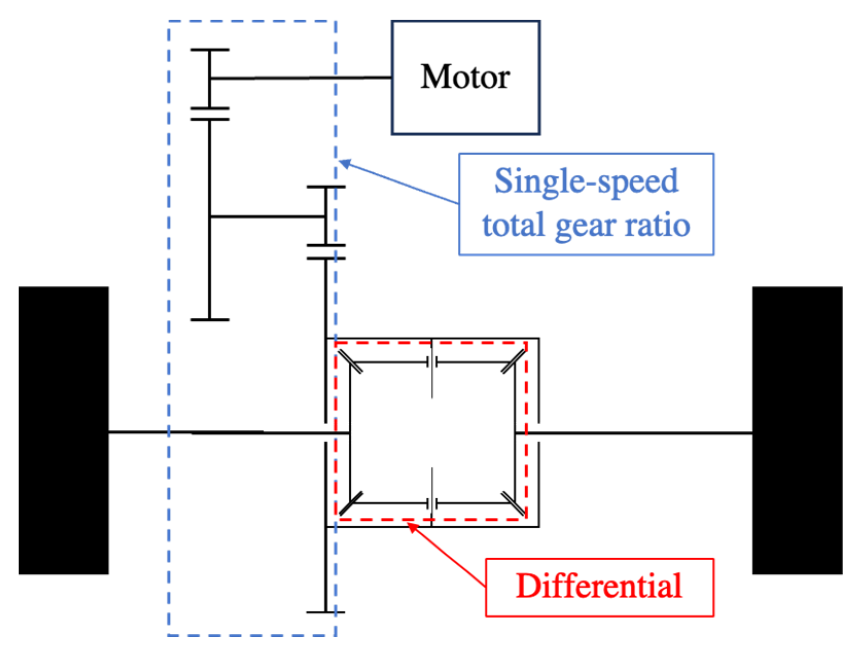
This model implements the single-speed reduction gear, including the effects of the differential.
Figure 6 shows a schematic of a single-speed transmission, which includes the single-speed total gear ratio group, composed of two single-stage gear mechanisms and the differential. The single-speed gear mechanism is composed of two gear sets arranged in series. The first gear set is usually called the gearbox gear and the second gear set is usually called the final reduction.
Using this transmission, a bijective relationship is imposed between the vehicle speed and the motor speed and between the torque at the vehicle wheel and the torque at the motor. Hence, no gearshift happens, which is usually a benefit in terms of comfort and shifting-related power losses, but no control on the efficiency related to the motor operating point (see
Figure 2 and
Figure 3) is given to the designer of the shifting strategy.
The output-to-input ratio of the rotational speed is a fixed value, the gears ratio, and the output power is equal to the input power minus the internal losses, which are evaluated as follows:
Regarding the single-speed total gear ratio group, an efficiency of 98% was considered for each gearset due to the gear meshing of the two single-stage gear sets.
Regarding the differential, an overall efficiency of 97% was considered, due to the engagement of the differential inner wheels and the lubrication losses.
The model also takes into account the bearing friction related to the shafts on which the gear wheels are mounted. The friction torque denoted as T was evaluated externally to the model using the following equation:
where
F represents the radial load acting on the bearing,
is the mean diameter of the bearing, and
f is the rolling friction coefficient of the bearing.
To calculate the radial force acting on the bearings, a system consisting of two meshing wheels, each fixed onto a shaft supported by a pair of bearings, was modeled. For each wheel, a diameter was chosen so that their division resulted in a value close to the gear ratio of the gear. With the known transmitted torque, it was possible to calculate the bearing reactions and thus the respective radial force acting on them. Once the friction torque is determined, the power losses can be evaluated as the product of the friction torque and the angular speed.
Note that the model allows power reversal, and therefore, it considers, when applying the losses, the correct flange as the input, e.g., the left one when in traction, the right when in regenerative braking.
2.3.4. Submodel “Inertias” (from the MSL)
This model, included in the MSL, combines the inertias of the rolling parts of lossyGear, differential, and wheels. Among these, the dominant term is due to the wheels and is still small. If converted into the translating mass, all rotating parts (including eleDrive) are equivalent to around 60–90 kg, in comparison with the total vehicle mass, which is around 1500–2200 kg, depending on the vehicle considered.
2.3.5. Submodel “Mass” (from MSL)
This is just a translating mass without any special feature.
2.3.6. Submodel “dragForce” (Created by us)
Since we only simulated the WLTC cycle, which does not consider any slope, the effects of the slope do not need to be included in the drag force model.
Our dragForce model uses the traditional binomial representation of the drag force (although better interpolation of the experimental data is obtained using a trinomial representation, e.g., also adding a term proportional to speed):
where
f is the rolling friction coefficient, usually between 0.011 and 0.014 in modern cars;
mg is the vehicle weight;
is the air density;
Cx is the aerodynamic drag coefficient which, in modern cars, is usually between 0.20 and 0.35;
S is the vehicle frontal area.
Note that the formula implies that, at zero speed, there is a force pushing the car in the reverse direction, which is unreal. Therefore, a different model for drag force is used for that case: the drag force will have to stay equal to the applied force up to the moment at which the vehicle starts moving (which, in turn, occurs when the applied force is overcome The advanced characteristics of Modelica language allow the creation of these kinds of hybrid models, where the behavior of the same object changes depending on the actual situation. Our model, therefore, is hybrid and includes this drag force behavior, although the details of the implementation are beyond this paper’s scope.
2.3.7. Submodel “Driver” (Created by Us)
In a vehicle, the driver is the master controller of the vehicle’s movement. Since just longitudinal movement was considered, only commands related to this movement were taken into consideration.
In order to follow the WLTC driving cycle, which sets the target speed at each time point, the driver has to just try to follow the target speed. For the purpose of this paper, therefore, a very reactive driver is an excellent choice, obtained here through a simple proportional controller with a very high gain. The driver receives the measured vehicle speed, which corresponds to a physical driver looking at the speedometer on the dashboard and acts on the accelerator and the brake pedal to adjust the actual speed to the reference speed given by the cycle.
In real-life vehicles, the powertrain tries to use the regenerative braking capability of the vehicle to the maximum extent possible. Only when very strong braking actions are needed or at very slow speeds (typically below 10 km/h), mechanical braking is used.
It is observed, however, that the WLTC implies smooth drive, and the required braking power usually never overcomes the maximum regeneration capability of the powertrain, and the substitution of the electrical braking with mechanical braking at very low speeds is conducted to enhance the efficiency, since at very low speeds, the electric drive train would require electric energy to brake, which is worse than just using mechanical brakes. This is because electric machines absorb power (“magnetization power”) just to generate the internal magnetic field necessary to brake; so, when the mechanical power is lower than the magnetizing power, during braking, the machine will absorb power from both the mechanical and electrical interfaces with the exterior.
But, the energy content at these very low speeds is very small in comparison to the vehicle’s kinetic energy at the average speed of the cycle. So, because of this, for BEV WLTC simulations, it is common to consider vehicles that always brake through the electrical drive train, and the results are good, as shown in
Section 3. It is also checked,
a- posteriori, that the required braking torque and power are compatible with the maximum capability of the electric drive.
2.4. The Two-Speed BEV Simulation Model
In general, it is possible to envisage BEVs with several speed gears, and these have been used in the past. For instance, the first Formula E cars had five-speed gears, and multiple speed gears have been proposed rather frequently in the literature [
4,
5,
6,
7]. In this paper, however, to find some basic results for real-life cars, we limited ourselves to two-speed gears. The two speed BEV simulation model has the appearance shown in
Figure 7.
Some of the submodels are the same as that shown in
Figure 1 and do not need an additional description here; we just describe the meaning and main purpose of the new sub-models:
Submodel “basicStrategy” (from library [
20])
This defines the strategy used to change speeds. Its output is an integer number defining the actual speed selected. It operates as a function of the vehicle speed and torque requested by the driver.
The details of the implemented strategy are reported in
Section 2.4.1.
Submodel “clutchControl” (from library [
20])
This model actuates the speed command received by the strategy and determines the activation of the correct clutch to select the desired speed. The block output is a vector signal. The end needs to be multiplexed before sending scalar signals to the dual-speed, dual-clutch gearbox.
Figure 8 shows a schematic of a dual-clutch transmission, composed of the dual-clutch total gear ratio group and the differential. The dual-clutch gear ratio group is composed of the dual-clutch package, connected to the engine and lubricated by oil, and two gear sets, connected to the first and second clutches, respectively. There is a common output shaft for both gear sets, and it is connected to the final reduction and to the differential, as in the single-speed gearbox. The first or second gear ratios can be selected by shifting the synchronizer to the left (1 gear) or to the right (2nd gear) and engaging the corresponding clutch.
The dual-clutch model is simply obtained by connecting a dual-clutch model (taken from the library [
20]), and two lossy gears, which are freely available in the Modelica Standard Library [
21], which implement the losses of the first and second gear sets, which are always rotating due to the common output shaft; the lossy gears also include the losses due to clutch lubrication.
Using this transmission, two gear ratios which determine two different relationships between the vehicle speed and the motor speed and between the torque at the vehicle wheel and the torque at the motor can be chosen. The gearshift is powershift (no power interruption between the motor and wheels during the gearshift maneuver) and usually automatic. The comfort is good if the shifting logic is well implemented, and two possible motor operating points exist for each vehicle state. This allows us to optimize the efficiency of the motor operating points, even if shifting losses occur. Hence, multiple consecutive gear shifting maneuvers should be avoided.
Regarding the clutch sizing, the values related to the number of discs and their size were chosen in a way that allows the clutch to transmit a torque of up to 1.4 times the maximum motor torque.
2.4.1. Gear Ratio Choice
For each vehicle, the two most efficient transmission ratios in terms of the fuel consumption were selected for the dual-clutch gearbox. This operation was performed in MathWorks Matlab R2023a
® [
23] through an optimization process: the efficiency of the transmission was written as a function of the transmission ratio
τ, from which a cost function was then formulated. Subsequently, for each time pointover the entire driving cycle, the value of
τ that minimized this cost function was determined, maximizing the transmission efficiency point-by-point throughout the entire cycle.
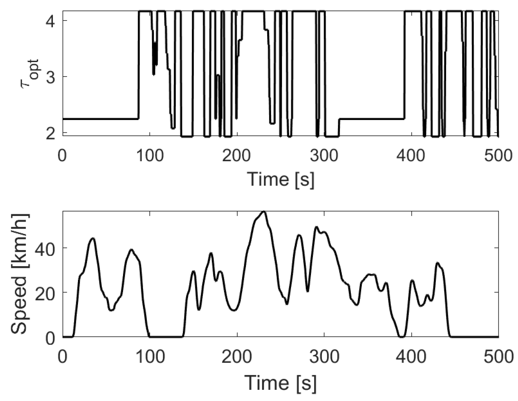
Figure 9 shows the trend of the optimal τ during the first 500 s of the WLTC cycle for vehicle T: the graph in the figure is the result of the optimization process described earlier that was carried out in Matlab
®.
Having obtained the trend of the optimal transmission ratio for energy consumption over the entire WLTC cycle, it is necessary to identify the two ratios with which to equip the transmission. To perform this, the two ratios that are repeated the most over the entire cycle were identified, and these were chosen as the two gear ratios for the transmission.
Table 2 shows the gear ratios selected for each vehicle.
2.4.2. Gear-Shift Strategy
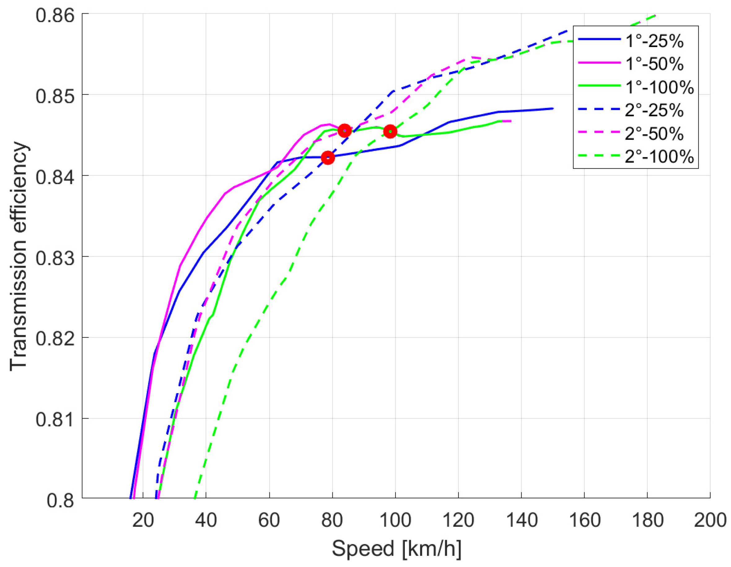
A gear-shifting strategy is necessary to control the dual-clutch gearbox. The variables that govern the gear shift are the vehicle’s speed and the percentage of throttle: for each transmission ratio and each throttle percentage, it is possible to evaluate the efficiency as a function of the vehicle speed. It is necessary, therefore, to determine which of the two gears is more efficient given the throttle value and the vehicle’s speed for a specific operating condition. So, as the speed and throttle percentage vary, the transmission efficiency trend was evaluated for both gears (
Figure 4 and
Figure 5): the shift from the first to the second gear occurs when, at a fixed throttle percentage, the efficiency curve for the second gear overcomes the curve of the first.
The red points presented in
Figure 10 and
Figure 11 identify the intersections between the two curves of the two gears for the same throttle percentage (for a clearer presentation of the figures, only the lines corresponding to three values of the throttle percentage are drawn): the interval to the right of the point indicates a region where the transmission is more efficient with the second reduction ratio.
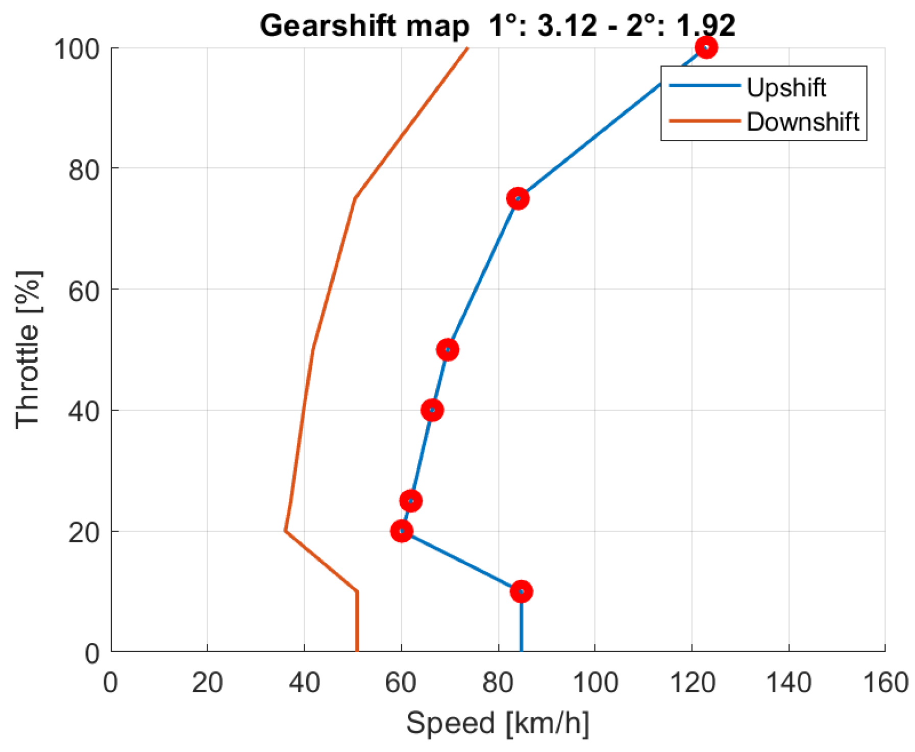
Figure 12 and
Figure 13 show the upshift curve for vehicles T and N obtained by connecting all points of intersection in the efficiency curves as the throttle value varied (all throttle percentage values are 10%, 20%, 25%, 40%, 50%, 75%, and 100%).
The downshift curve was chosen according to [
6] to avoid gear hunting, which is unnecessary and repeated gear shifting.
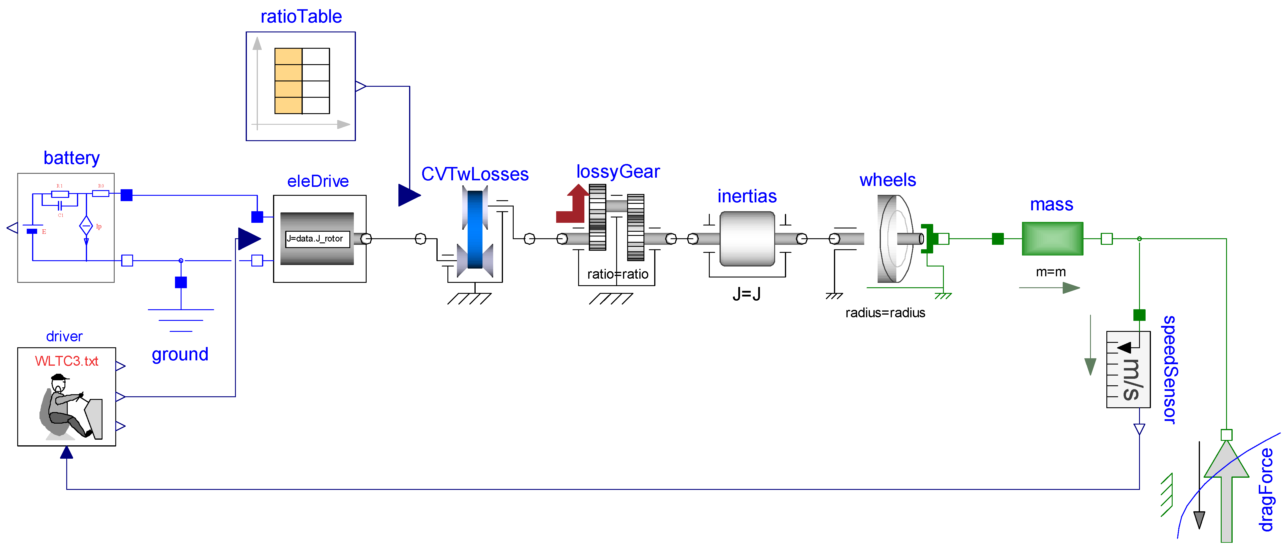
2.5. The CVT BEV Simulation Model
A second version of a BEV with adjustable speed ratio transmission was considered. This contains CVT (continuously variable transmission).
Figure 14 shows a schematic of CVT, composed of the CVT total gear ratio group and the differential. CVT is composed of two pulleys and one trapezoidal belt. The winding radius of the belt on each pulley is obtained by changing the axial distance between the semi-pulleys of the primary and secondary pulleys in order to materialize the desired gear ratio. The secondary pulley is connected to the final gear ratio and, consequently, to the differential, as in the single-speed transmission and in the dual-clutch transmission.
Using this transmission, ideally, infinite gear ratios should be obtained within a given range of values. Hence, infinite relationships exist between the vehicle operating point and the motor operating point. The gearshift is powershift (no power interruption between the motor and wheels during the gearshift maneuver) and automatic. The comfort is good if the shifting logic is well-implemented, and infinite possible motor operating points exist for each vehicle state. This allows us to optimize the efficiency of the motor operating points, even if the efficiency of the transmission itself is low, especially during gear shifting. Hence, multiple consecutive gear shifting maneuvers should be avoided. The vehicle model is similar to the ones previously described and is shown in
Figure 15.
The only meaningful difference in comparison with the model presented in
Figure 4 is the presence of CVTwLosses instead of the dual-clutch transmission. When the speed ratio changes, however, there are additional losses due to increased sliding. The CVT losses have been taken into account through the model proposed in [
24].
The submodel CVTwLosses receives the gear ratios to be actuated as the input, as taken from a ratio table, which contains the ratios as a function of time; these ratios were determined prior to the simulation according to the strategy presented below.
Below are the main parameters considered in the development of the two transmission models:
Gear Ratio: Regarding the DCT model, the gear ratios selected for each vehicle are reported in
Table 2. As for the CVT model, the transmission ratio can vary continuously within the range of 4.2 to 1.9 for vehicle T and 3 to 0.9 for vehicle N.
Friction: The DCT model considers viscous losses due to the action of the lubricant on the clutch discs. The CVT model takes into account the friction torque due to belt slip on the pulleys. This torque is proportional to the transmitted torque and the gear ratio.
Controller: In the DCT model, the controller chooses the most efficient transmission ratio considering the vehicle speed and the percentage of the accelerator at that specific driving moment. Regarding the CVT model, the gear ratio is selected by a table that imposes the most efficient transmission ratio for the specific driving conditions at each simulation instant.
Gear-Shift Strategy: The trend of the optimal transmission ratio during the WLTC cycle was obtained using the method already shown in
Section 2.3.1 for selecting the gears of the two-speed model. A post-processing activity was conducted on the obtained profile to achieve a new transmission ratio trend. Losses associated with the CVT occur both when the transmission ratio changes but also with a fixed gear ratio. Therefore, the
τ profile was adjusted by attempting to eliminate unnecessary gear shifts between transmission ratios close to each other, which do not bring efficiency benefits to the transmission but introduce losses. The optimal profile was found through a trial-and-error process by eliminating gear shifts between two transmission ratios that are closer to each other by a certain fixed value Δ
τ.
2.6. The WLTC
In recent years, a proposed worldwide standard for the verification of performances of light duty vehicles was introduced and named the Worldwide Light-Duty Test Cycle WLTC. In conjunction with this cycle, specifications on how to cover this cycle have been introduced; therefore, the cycle is commonly known as the Worldwide Light-Duty Test Procedure (WLTP), including the test cycle and procedures with this acronym. The EU has adopted this procedure and cycle for homologation, and it is currently used for every rolls-bench homologation.
Since this cycle is considered an international standard, it was therefore used in this paper, in particular, in version 3b, which refers to light vehicles with power-to-mass ratios above 34 W/kg and maximum speeds above 120 km/h, a class to which the considered cars belong. The cycle is a speed versus time profile, with the appearance shown in
Figure 16. The average speed is 46.5 km/h, and the cycle mainly refers to urban and suburban paths; only the last 300 s (extra high-speed phase) has motorway-like speeds (which explains why BEV users frequently complain that the real-life consumptions are much larger than those of homologation: if they refer to the motorway run, this is obviously due to the large drag force we have at high speeds, see Equation (1)).
3. Results
3.1. Vehicle Efficiency
As described in
Section 2.1, all submodel data were taken from trustworthy literature papers. In a few cases, some missing data were defined considering reasonable values for the vehicles under consideration.
However, as a final validation of the global performance of the obtained vehicle models, we checked the total electricity consumption under the WLTC of the vehicles with available data. The results of this comparison are shown in
Table 3.
The simulation data are not totally in line with those of the manufacturer, also considering that the latter should be those from homologation, which, in turn include battery and recharge losses, which are not included in the simulation results.
However, this discrepancy does not surprise us much, since the assumed vehicle data come from different sources, some of which are independent of the manufacturer, and therefore, their consistency is limited.
Nevertheless, two realistic vehicles were obtained, where T was larger than N, making them adequate for use to compare different mechanical transmission systems.
3.2. The Single-Speed Ratio for Maximum Efficiency
For a given electric drive and vehicle chassis, the final reduction gear of a BEV can be chosen by pursuing the maximum efficiency, i.e., the minimum Wh/km consumption. This, however, may not give an easily marketable performance.
The data assumed for vehicles T and N bring enough efficiency, but not the maximum possible.
Table 4 compares the results obtained using the assumed reduction gears and the minimum consumption (“efficient”) ones. Obviously, the efficient ratios were verified to be such that the WLTC cycle was correctly covered, given the torque speed and power constraints of the powertrain. It is also observable that the improvement in efficiency led to a significant reduction in the vehicle’s acceleration.
In the remainder of this paper, comparisons between mechanical transmissions using vehicles equipped with the literature reduction ratios are made.
3.3. Consumption Evaluation at Equal Performances
Table 5 shows a comparison of the simulation results related to the consumption and acceleration values for vehicles T and N with the different transmissions considered. In the column related to consumption, the percentage decrease in vehicle fuel consumption on the WLTC cycle equipped with DCT (dual-clutch transmission) and CVT is reported compared to the original fixed-ratio model, that is, the one found in real vehicles. The original gear ratios used in single-speed transmission were taken from the literature and are indicated in
Table 4, so as to guarantee the vehicle design performance.
Concerning DCT, the considered gear ratios were obtained considering the procedure described in
Section 2.4.1. and the values found
Table 2, which allow us to minimize the total consumption during the WLTC driving cycle. The gear shifting is automated and follows the strategy described in
Section 2.4.2. Also, for the CVT, the gear shifting is automated, and the shifting strategy is as described in
Section 2.5.
The results demonstrate that the two new solutions can improve the powertrain efficiency compared to the original single-speed transmission. Specifically, CVT stands out as the transmission that ensures the best energy efficiency: it allows for 7.42% and 7.00% reductions in energy consumption (respectively, for vehicles T and N), compared to the 5.57% and 3.76% saved by DCT. Additionally, the increase in efficiency occurs, with respect to the previous case by increasing the original vehicle performance. This is because it allows us to enlarge the constant power zone in the vehicle–speed–traction force plane in comparison with what is available in the rotational speed–torque plane (used in
Figure 1 and
Figure 3).
Figure 17 and
Figure 18 show the electric drive operating points on the efficiency map for both vehicles.
Figure 17 shows the benefits of the two-speed transmission and CVT for vehicle T: DCT allows the shifting of some points from a low torque or speed, i.e., low-efficiency areas, towards regions with higher torque and efficiency values.
Figure 18 shows similar results for vehicle N: some operating points move away from the low-efficiency regions at the bottom of the map for DCT, whereas CVT allows the electric drive to work more on the high-power regions corresponding to higher efficiencies. Note that the trajectory is traced by joining the operating points with straight lines, and in some cases, subsequent points are far away from each other. Since transition from a CVT ratio to the next one is simulated as being instantaneous, the intermediate points along these lines are not actual operating points; this occurs, for instance, when the straight lines traverse the area above the maximum electric drive power in
Figure 18.
Figure 19 and
Figure 20 show the energy consumption for both vehicles in the four different phases of the WLTC cycle: the graphs show that, for both the two-speed transmission and CVT, for both vehicles, the overall decrease in energy consumption over the entire cycle is due to a decrease in consumption in all four phases. For vehicle T, considering DCT, there is a relatively constant reduction in energy consumption across the four different phases, ranging from 5.3% to 6%. A similar situation occurs for CVT, where the reduction in consumption varies from 6.1% to 8.6%. The situation is different for vehicle N, where the consumption reduction varies across phases, ranging from a 1.9% decrease in the ‘medium’ phase to a 4.3% decrease in the ‘extra high’ phase for DCT. Regarding CVT, it also varies from a 1.2% reduction in the ‘medium’ phase to a 9.3% decrease in the ‘extra igh’ phase. These data are reflected in the overall reduction in consumption reported in
Table 5.
4. Discussion
To evaluate the value of adding multi-speed transmission to the electric vehicles, the increased manufacturing cost and the reduced daily-use cost are calculated in the following cost–benefit analysis.
In [
25], the relative selling price (RSP) method is proposed to evaluate the economic weight of the new solutions with Equation (3). The RSP index allows us to calculate the increase in costs related to the new transmissions compared to the single-speed reducer whose cost is set to zero in this analysis.
In Equation (3), is the maximum ratio, is the motor’s maximum output torque, and is the number of gears. The selling price of the belt CVT is estimated to be similar to that of a six-speed automatic transmission, so is set to be equal to 6.
The estimated gearbox relative selling prices are presented in
Table 6. It can be considered that vehicles T and N belong to car segments E and B, respectively, as shown in [
25].
At this point, to evaluate the overall cost of the transmission, the obtained RSP value is multiplied by the unit cost of the transmission . The economic savings achieved by the new transmissions are mainly due to two factors:
- 1.
The improved efficiency of the new transmissions allows, for the same driving range, the vehicles to be equipped with a battery pack with a lower energy capacity, saving on this component. The capacity
of the new battery is obtained by multiplying the original vehicle’s range
R by its energy consumption in Wh/km with the new transmission. The new battery capacities are, therefore, shown in
Table 7.
At this point, considering the cost of the battery pack , it is then possible to evaluate the achieved savings.
- 2.
The lower vehicle consumption due to the new transmissions clearly reduces the amount of energy consumed and therefore the related costs over the entire lifespan of the vehicle. Specifically, given the value
for the vehicle’s lifespan, the relative efficiency of the charging process
, and the cost of electrical energy
, the cost related to the consumed energy
during the vehicle’s lifespan is obtained with Formula (4):
In
Table 8, the values used in the formulas for the calculations just shown are provided. In particular, to conduct a realistic analysis, a price range between a maximum value and a minimum value was considered for the battery and electrical energy costs. Regarding the battery costs, [
26] states that these prices are trending towards values lower than 200 €/kWh. We decided to consider a range between 150 and 200 €/kWh for this price, which is highly dependent on market fluctuations. As for electricity costs, we considered a range between the values of 0.25 and 0.70 €/kWh, respectively, for domestic and public charging costs.
Regarding the transmission costs, [
25] uses the values written in
Table 6 for E-Class and B-Class vehicles.
A charging process efficiency value of 0.9 is reported in the table. This was obtained as the product of the charger device’s efficiency and the battery charging efficiency, both considered to be 0.95.
Table 9 presents the cost balance of the transmissions:
For both vehicles, the first column shows the capital cost (CC), which is the sum of the savings on the battery, which are higher in the case of the highest considered quotation (e.g., 200 €/kWh), and the additional costs of the transmissions, which are fixed for each considered technology (e.g., DCT or CVT); this affects the initial cost of the vehicle.
The second column shows the running cost (RC), representing the savings due to lower energy consumption during the vehicle’s lifespan.
The sum of these two items determines the total cost (TC), shown in the third column.
The results show that the studied transmissions have an economic benefit in terms of the total cost, except for one case in which vehicle T is equipped with CVT. Regarding CVT, the high initial cost is balanced by the significant energy savings during the cycle, thus resulting in substantial overall cost savings.
For both vehicles, when considering the costs related to public charging, e.g., 0.70 €/kWh, a significant total cost reduction was achieved, which was in the range of 1.5–2.0 k€ for all examined configurations, except for vehicle N with dual-clutch transmission. On the other hand, when charging at home, the economic benefit drops to a few hundred euros, except for vehicle T equipped with CVT, over the whole lifespan.
When comparing the results to the existing literature, the cost–benefit analysis conducted by [
25] leads to greater economic savings due to the higher battery cost considered: the article refers to a battery cost of 400
$/kWh, the right price in 2018, and in this way, the economic benefit due to the smaller battery pack being excessive.
Considering the values used in the
Table 8, the analysis conducted by [
25] leads to results like those shown in
Table 9.
As a further consideration, the significance of this research is mainly related to the future market of BEVs, since today’s manufacturers tend to reduce building costs as much as possible. These are still higher for BEVs with respect to ICEV. This corresponds to very high purchase costs, which make it difficult to introduce new technologies onboard, and a reduction in operating costs is less important from the user point of view. On the other hand, against further building cost reductions, manufacturers will have the possibility to invest in additional technical aspects, like those presented in this paper. The users, being able to purchase BEVs at a reduced cost, will be much more focused on solutions aimed at reducing the operating costs.
5. Conclusions
The simulations performed show that the usage of multiple-gear transmission, either dual-clutch two speed or CVT, is able to increase the competitiveness of BEVs, because the advantages in terms of efficiency reductions overcompensate for the additional costs due to the addition of variable-speed transmissions. This almost always occurs in the case of the two cars considered in this paper at the current and future costs of components, with economic and expensive electricity values.
In particular, the maximum saving cost achieved across the whole vehicle lifespan was slightly below 2 k€, with the CVT solution, the highest battery price, e.g., 200 €/kWh, and electrical energy, e.g., 0.70 €/kWh. Savings reduced by about one order of magnitude when considering the lowest costs for electricity and batteries, e.g., 150 €/kWh and 0.25 €/kWh respectively.
However, the use of DCT and CVT increases vehicle capital costs by about 0.5 and 1.0 k€, respectively, thus representing one significant barrier to BEV diffusion, and this could be one of the causes of their very low use nowadays.
Finally, it also increases dynamic performance (i.e., acceleration between 0 and 100 km/h). In this case, the CVT solution is able to reduce the acceleration time by about 1 s, while DCT stops at a reduction of approximately 0.2 s.
The results shown in this paper were obtained using Modelica models, which can be simulated through the open-source, freely available Modelica simulation tool [
18].
The models containing DCT and CVT cannot be disclosed, since they contain parts that are copyrighted. The model of the single-speed gears is instead freely available, since it is published in folder “MDPI Vehicles paper 2023” in the repository
https://github.com/ceraolo/ModelicaPaperModels (accessed on 10 November 2023), where information on how to use it is also provided. The model’s appearance is very similar to this paper’s figures; it just contains a few more self-explanatory elements, which were dropped from this paper’s figures to make them simpler.
The reader can freely repeat the simulations proposed in this paper, as well as study variations in the vehicles (e.g., changing mass, rolling friction coefficient, gear ration, etc.) or study completely different BEVs at will.
In the same archive, a brief explanation on how to use the model to reproduce the paper’s results and obtain new results with modified data is included.
Because of the modular and open characteristic of Modelica language, the user can also try to add the missing parts and build their own models, based on the information in the text, to also replicate simulations with DCT or CVT.
Author Contributions
Conceptualization, M.C. and F.F.; methodology, F.B. and G.L.; software, E.B. and M.C.; validation, E.B. and M.C.; formal analysis, M.C., F.B., F.F. and G.L.; investigation, F.B. and E.B.; resources, M.C.; data curation, E.B., F.B. and G.L.; writing—original draft preparation, E.B. and M.C.; writing—review and editing, E.B., M.C., F.B., F.F. and G.L.; visualization, M.C., F.B., F.F., E.B. and G.L.; supervision, M.C. and F.F.; project administration, M.C.; funding acquisition, M.C. All authors have read and agreed to the published version of the manuscript.
Funding
This study was carried out within the MOST—Sustainable Mobility Center and received funding from the European Union Next-Generation EU (piano nazionale di ripresa e resilienza (PNRR)—missione 4 componente 2, investimento 1.4—d.d. 1033 17/06/2022, cn00000023). This manuscript reflects the authors’ views and opinions only; neither the European Union, nor the European Commission can be considered responsible for them.
Data Availability Statement
All data used for the study data were taken from the literature, as detailed in the main text.
Conflicts of Interest
The authors declare no conflict of interest.
References
- Pasini, G.; Lutzemberger, G.; Ferrari, L. Renewable Electricity for Decarbonisation of Road Transport: Batteries or E-Fuels? Batteries 2023, 9, 135. [Google Scholar] [CrossRef]
- BMalozyomov, V.; Martyushev, N.V.; Konyukhov, V.Y.; Oparina, T.A.; Zagorodnii, N.A.; Zagorodnii, E.A.; Qi, M. Mathematical analysis of the reliability of modern trolleybuses and electric buses. Mathematics 2023, 11, 3260. [Google Scholar] [CrossRef]
- Pamula, T.; Pamula, D. Prediction of electric buses energy consumption from trip parameters using deep learning. Energies 2022, 15, 1747. [Google Scholar] [CrossRef]
- Ren, Q.; Crolla, D.A.; Morris, A. Effect of Transmission Design on Electric Vehicle (EV) Performance. In Proceedings of the IEEE Vehicle Power and Propulsion Conference, Dearborn, MI, USA, 7–11 September 2009. [Google Scholar]
- EU Regulation 2017/1151. Available online: https://eur-lex.europa.eu/legal-content/EN/TXT/?uri=celex%3A32017R1151 (accessed on 10 November 2023).
- Bottiglione, F.; de Pinto, S.; Manriota, G.; Sorniotti, A. Energy Consumption of a Battery Electric Vehicle with Infinitely Variable Transmission. Energies 2014, 7, 8317–8337. [Google Scholar] [CrossRef]
- Ruan, J.; Walker, P.; Zhang, N. A comparative study energy consumption and costs of battery electric vehicle transmissions. Appl. Energy 2016, 165, 119–134. [Google Scholar] [CrossRef]
- Latinen, H.; Lajunen, A.; Tammi, K. Improving Electric Vehicle Energy Efficiency with Two-Speed Gearbox. In Proceedings of the IEEE Vehicle Power and Propulsion Conference, Belfort, France, 11–14 December 2017. [Google Scholar]
- Tesla Technical Data. Available online: https://www.tesla.com/en_eu/support/european-union-energy-label (accessed on 10 November 2023).
- Tesla Technical Data. Available online: https://www.tesla.com/sites/default/files/blog_attachments/the-slipperiest-car-on-the-road.pdf (accessed on 10 November 2023).
- Tesla Technical Data. Available online: https://www.evspecifications.com/en/model/39812e (accessed on 10 November 2023).
- Nissan Technical Data. Available online: https://www.nissan.it/veicoli/veicoli-nuovi/leaf.html (accessed on 10 November 2023).
- Nissan Technical Data. Available online: https://www.evspecifications.com/en/model/b1e92 (accessed on 10 November 2023).
- Popescu, M.; Goss, J.; Staton, D.; Hawkins, D.; Chong, Y.C.; Boglietti, A. Electrical Vehicles-Practical Solutions for Power Traction Motor Systems. IEEE Trans. Ind. Appl. 2018, 54, 2751–2762. [Google Scholar] [CrossRef]
- Baumgartner, F.P.; Schmidt, H.; Burger, B.; Bründlinger, R.; Häberlin, H.; Zehner, M. Status and relevance of the DC voltage dependency of the inverter efficiency. In Proceedings of the 22nd European Photovoltaic Solar Energy Conference and Exhibition, Milan, Italy, 3–7 September 2007. [Google Scholar]
- Online Book ModelicaByExample. Available online: https://mbe.modelica.university/ (accessed on 10 November 2023).
- Fritzson, P. Principles of Object-Oriented Modeling and Simulation with Modelica 3.3: A Cyber-Physical Approach, 2nd ed.; Wiley: Hoboken, NJ, USA, 2014; ISBN 9781118859124. [Google Scholar]
- Full List of Modelica Libraries. Available online: https://modelica.org/libraries/ (accessed on 10 November 2023).
- OpenModelica. Available online: www.openmodelica.org (accessed on 10 November 2023).
- Commercial Modelica Library PowerTrain, Developed by DLR Institute of Systems Dynamic and Control. Available online: https://www.claytex.com/products/dymola/model-libraries/vesyma/powertrain/ (accessed on 10 November 2023).
- Modelica Standard Library, Free Library Distributed with Modelica Simulation Tools. Available online: https://github.com/modelica/ModelicaStandardLibrary (accessed on 10 November 2023).
- Barbieri, M.; Ceraolo, M.; Lutzemberger, G.; Scarpelli, C. An Electro-Thermal Model for LFP Cells: Calibration Procedure and Validation. Energies 2022, 15, 2653. [Google Scholar] [CrossRef]
- Official Website for Matlab. Available online: www.mathworks.com (accessed on 10 November 2023).
- Lei, Y.L.; Jia, Y.Z.; Fu, Y.; Liu, K.; Zhang, Y.; Liu, Z.J. Car Fuel Economy Simulation Forecast Method Based on CVT Efficiencies Measured from Bench Test. Chin. J. Mech. Eng. 2018, 31, 83. [Google Scholar] [CrossRef]
- Ruan, J.; Walker, P.D.; Wu, J.; Zhang, N.; Zhang, B. Development of continuously variable transmission and multi-speed dualclutch transmission for pure electric vehicle. Adv. Mech. Eng. 2018, 10, 1–15. [Google Scholar] [CrossRef]
- Nykvist, B.; Sprei, F.; Nilsson, M. Assessing the progress toward lower priced long range battery electric vehicles. Energy Policy 2019, 124, 144–155. [Google Scholar] [CrossRef]
Figure 1.
Vehicle N’s electric drive efficiency map.
Figure 1.
Vehicle N’s electric drive efficiency map.
Figure 2.
Vehicle T’s motor efficiency map.
Figure 2.
Vehicle T’s motor efficiency map.
Figure 3.
Vehicle T’s electric drive efficiency map.
Figure 3.
Vehicle T’s electric drive efficiency map.
Figure 4.
Diagram of the single-speed BEV simulation model.
Figure 4.
Diagram of the single-speed BEV simulation model.
Figure 5.
Diagram of the “eleDrive” model.
Figure 5.
Diagram of the “eleDrive” model.
Figure 6.
Schematic of a single-speed gear.
Figure 6.
Schematic of a single-speed gear.
Figure 7.
Diagram of the two-speed BEV simulation model.
Figure 7.
Diagram of the two-speed BEV simulation model.
Figure 8.
Schematic of the dual-clutch transmission.
Figure 8.
Schematic of the dual-clutch transmission.
Figure 9.
Optimal transmission ratio τ trend for vehicle T in the first 500 s.
Figure 9.
Optimal transmission ratio τ trend for vehicle T in the first 500 s.
Figure 10.
Transmission efficiency for the two gears selected for vehicle T.
Figure 10.
Transmission efficiency for the two gears selected for vehicle T.
Figure 11.
Transmission efficiency for the two gears selected for vehicle N.
Figure 11.
Transmission efficiency for the two gears selected for vehicle N.
Figure 12.
Vehicle T’s gearshift map.
Figure 12.
Vehicle T’s gearshift map.
Figure 13.
Vehicle N’s gearshift map.
Figure 13.
Vehicle N’s gearshift map.
Figure 14.
Schematic of CVT.
Figure 14.
Schematic of CVT.
Figure 15.
Diagram of the CVT BEV simulation model.
Figure 15.
Diagram of the CVT BEV simulation model.
Figure 16.
The WLTC test cycle.
Figure 16.
The WLTC test cycle.
Figure 17.
Comparison between the operating points of the original gear ratio and DCT (left) and CVT (right) on the electric drive efficiency map for vehicle T.
Figure 17.
Comparison between the operating points of the original gear ratio and DCT (left) and CVT (right) on the electric drive efficiency map for vehicle T.
Figure 18.
Comparison between the operating points of the original gear ratio and DCT (left) and CVT (right) on the electric drive efficiency map for vehicle N.
Figure 18.
Comparison between the operating points of the original gear ratio and DCT (left) and CVT (right) on the electric drive efficiency map for vehicle N.
Figure 19.
Comparison between the energy consumption of the original transmission and DCT (left) and CVT (right) for vehicle T in the four different phases of the WLTC cycle.
Figure 19.
Comparison between the energy consumption of the original transmission and DCT (left) and CVT (right) for vehicle T in the four different phases of the WLTC cycle.
Figure 20.
Comparison between the energy consumption of the original transmission and DCT (left) and CVT (right) for vehicle N in the four different phases of the WLTC cycle.
Figure 20.
Comparison between the energy consumption of the original transmission and DCT (left) and CVT (right) for vehicle N in the four different phases of the WLTC cycle.
Table 1.
Vehicle data.
| Parameter | Description | Values | Units |
|---|
| | | T | N | |
|---|
| m | Vehicle mass | 2099 | 1643 | kg |
| Total gear ratio | 9.734 | 7.938 | - |
| Differential gear ratio | 3.12 | 4.353 | - |
| Tire radius | 0.3525 | 0.3162 | m |
| Aerodynamic drag coefficient | 0.24 | 0.29 | - |
| S | Frontal area | 2.34 | 2.28 | |
| Maximum output power | 225 | 80 | kW |
| Maximum output torque | 430 | 280 | Nm |
| Maximum motor speed | 1571 | 1088 | rad/s |
| Rolling friction coefficient | 0.013 | - |
Table 2.
Selected transmission ratios for the two vehicles.
Table 2.
Selected transmission ratios for the two vehicles.
Table 3.
Comparison of simulation and literature-specific consumption values (Wh/km).
Table 3.
Comparison of simulation and literature-specific consumption values (Wh/km).
| Vehicle | Energy Consumption (WLTC) |
|---|
| | Simulation | Reference | Source |
|---|
| T | 182.5 | 175 | [9] |
| N | 159.9 | 171 | [12] |
Table 4.
Comparison of simulated and literature-specific WLTC consumption and acceleration.
Table 4.
Comparison of simulated and literature-specific WLTC consumption and acceleration.
| | Data | Results |
|---|
| Vehicle | | Gear Ratio * | Wh/km | 0–100 km/h (s) |
|---|
| T | Literature | 9.734 | 182.5 | 6.54 |
| Efficient | 6.000 | 179.0 | 9.92 |
| N | Literature | 7.938 | 159.9 | 12.01 |
| Efficient | 5.500 | 156.9 | 13.81 |
Table 5.
Comparison of the simulation’s WLTC consumption and acceleration.
Table 5.
Comparison of the simulation’s WLTC consumption and acceleration.
| | | Results |
|---|
| Vehicle | | Wh/km | 0–100 km/h (s) |
|---|
| T | Original | 182.5 | 6.54 |
| DCT * | 172.4 (−5.57%) | 6.31 |
| CVT ** | 169.0 (−7.42%) | 5.50 |
| N | Original | 159.9 | 12.01 |
| DCT | 153.9 (−3.76%) | 11.81 |
| CVT | 148.7 (−7.00%) | 10.91 |
Table 6.
Estimated gearbox relative selling prices.
Table 6.
Estimated gearbox relative selling prices.
| | Two-Speed (DCT) | CVT |
|---|
| T (E-Class) | 0.87 | 1.34 |
| N (B-Class) | 0.53 | 0.91 |
Table 7.
New battery capacities [kWh] and their reductions compared with the original ones.
Table 7.
New battery capacities [kWh] and their reductions compared with the original ones.
| | T | N |
|---|
| DCT * | 56 (−4) | 23 (−1) |
| CVT ** | 55 (−5) | 22 (−2) |
Table 8.
Parameters used in the cost–benefit analysis.
Table 8.
Parameters used in the cost–benefit analysis.
| Parameter | Description | Values | Units |
|---|
| Battery cost | 150–200 | €/kWh |
| (E-Class) | Transmission cost (E-Class) | 12.5 | €/kW |
| (B-Class) | Transmission cost (B-Class) | 9.5 | €/kW |
| Energy cost | 0.25–0.70 | €/kWh |
| Vehicle’s lifetime range | 250,000 | km |
| Charging efficiency | 0.9 | - |
Table 9.
Cost increase [€] for each type of transmission and vehicle.
Table 9.
Cost increase [€] for each type of transmission and vehicle.
| | | | T | N |
|---|
| | Battery [€/kWh] | Energy [€/kWh] | CC | RC | TC | CC | RC | TC |
|---|
| DCT | 150 | 0.25 | +590 | −704 | −114 | +371 | −416 | −45 |
| 0.70 | +590 | −1970 | −1380 | +371 | −1166 | −795 |
| 200 | 0.25 | +423 | −704 | −281 | +352 | −416 | −91 |
| 0.70 | +423 | −1970 | −1547 | +352 | −1166 | −841 |
| CVT | 150 | 0.25 | +1009 | −939 | +70 | +611 | −775 | −164 |
| 0.70 | +1009 | −2628 | −1619 | +611 | −2169 | −1558 |
| 200 | 0.25 | +786 | −939 | −153 | +527 | −775 | −248 |
| 0.70 | +786 | −2628 | −1842 | +524 | −2169 | −1642 |
| Disclaimer/Publisher’s Note: The statements, opinions and data contained in all publications are solely those of the individual author(s) and contributor(s) and not of MDPI and/or the editor(s). MDPI and/or the editor(s) disclaim responsibility for any injury to people or property resulting from any ideas, methods, instructions or products referred to in the content. |
© 2023 by the authors. Licensee MDPI, Basel, Switzerland. This article is an open access article distributed under the terms and conditions of the Creative Commons Attribution (CC BY) license (https://creativecommons.org/licenses/by/4.0/).

 ,
, 


