Machine-Learning-Based Digital Twins for Transient Vehicle Cycles and Their Potential for Predicting Fuel Consumption

Abstract

Transient car emission tests generate huge amount of test data, but their results are usually evaluated only using their “accumulated” cycle values according to the homologation limits. In this work, two machine learning models were developed and applied to a truck RDE test and two light-duty vehicle chassis emission tests. Different from the conventional approach, the engine parameters and fuel consumption were acquired from the Engine Control Unit, not from the test measurement equipment. Instantaneous engine values were used as input in machine-learning-based digital twins. This novel approach allows for much less costly vehicle tests and optimizations. The paper’s novel approach and developed digital twins model were able to predict both instantaneous and accumulated fuel consumption with good accuracy, and also for tests cycles different to the one used to train the model.

1. Introduction

To reduce vehicle emissions and fuel consumption, manufacturers invest enormous resources for developing different strategies and methodologies to increase the efficiency of vehicles. Some strategies do not require substantial hardware modification, such as the introduction of low viscosity/friction engine oils [1,2,3,4,5,6,7,8,9,10,11,12,13,14,15,16,17]. Fuel savings with improved oil formulations in the order of 1 to 3% [8,9,11] are evaluated by specific test protocols such as the API sequence VI-A, Mercedes Benz M111 and ECE-15 cycle for truck chassis [11]. For these, costly hardware and test programs are needed since the impact of oil formulation and other engine components on fuel consumption is of same magnitude of experimental measurement deviations in fuel consumption.

Computer and/or empirical models are usually used to predict individual contributions prior to more expensive engine and vehicle tests; see for example [11,13,14,15,16]. During engine development, numerical models are used for optimizing fuel consumption (as well as other parameters). Such models can be divided into two main categories:

• Physical-based models: the system physics is described with mathematical equations. Extensive know-how and a theoretical background are usually required to obtain reliable and useful models. A trade-off between CPU consumption and model details is frequently found. These models can range from a detailed subsystem of the engine using 3D CFD to study an accurate solution that then is extrapolated to the whole engine [18,19] to a 1D/0D model offering a lower computational cost, but also lower details of the problem’s physics for reducing fuel consumption [11,16,17,20,21].
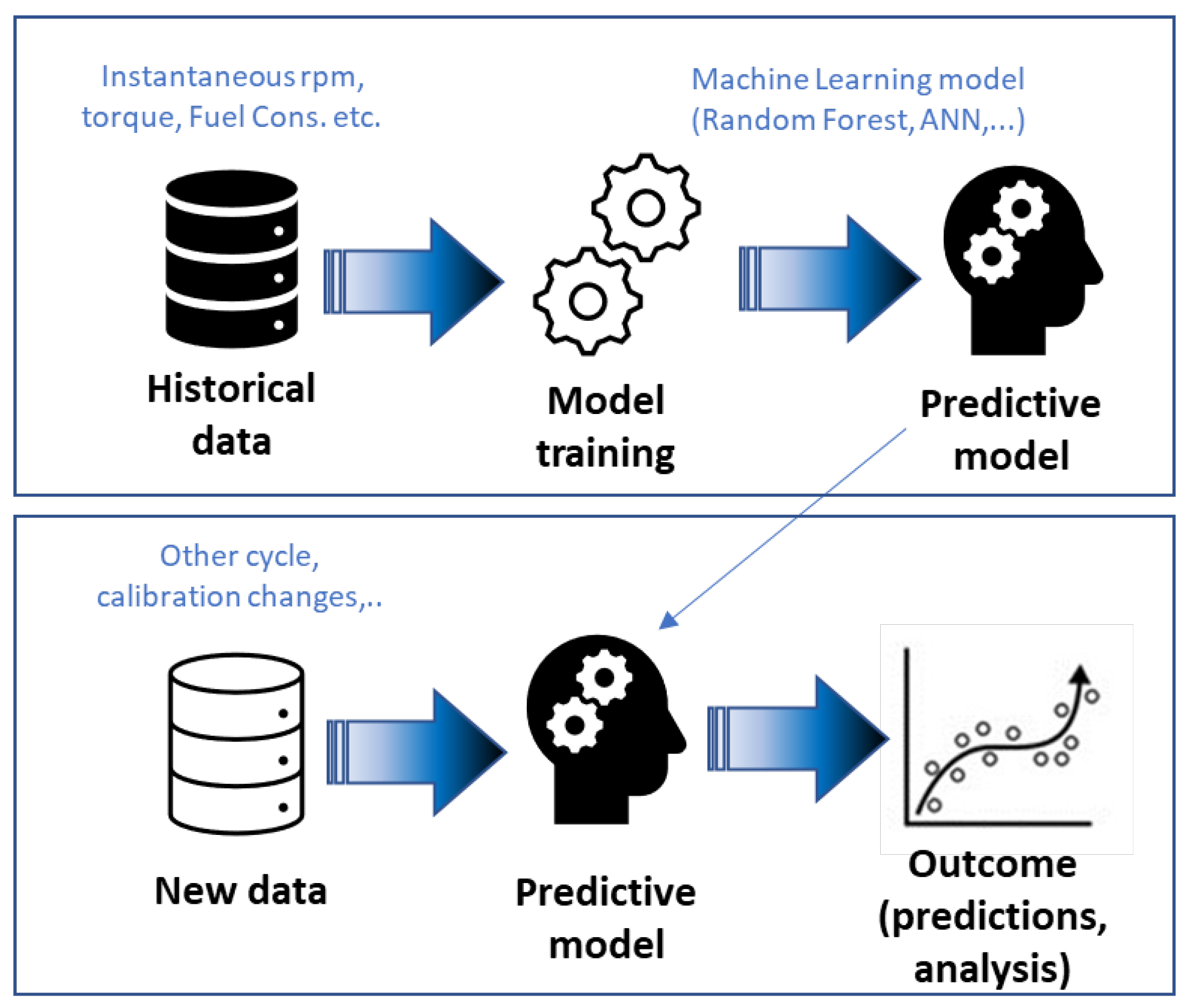
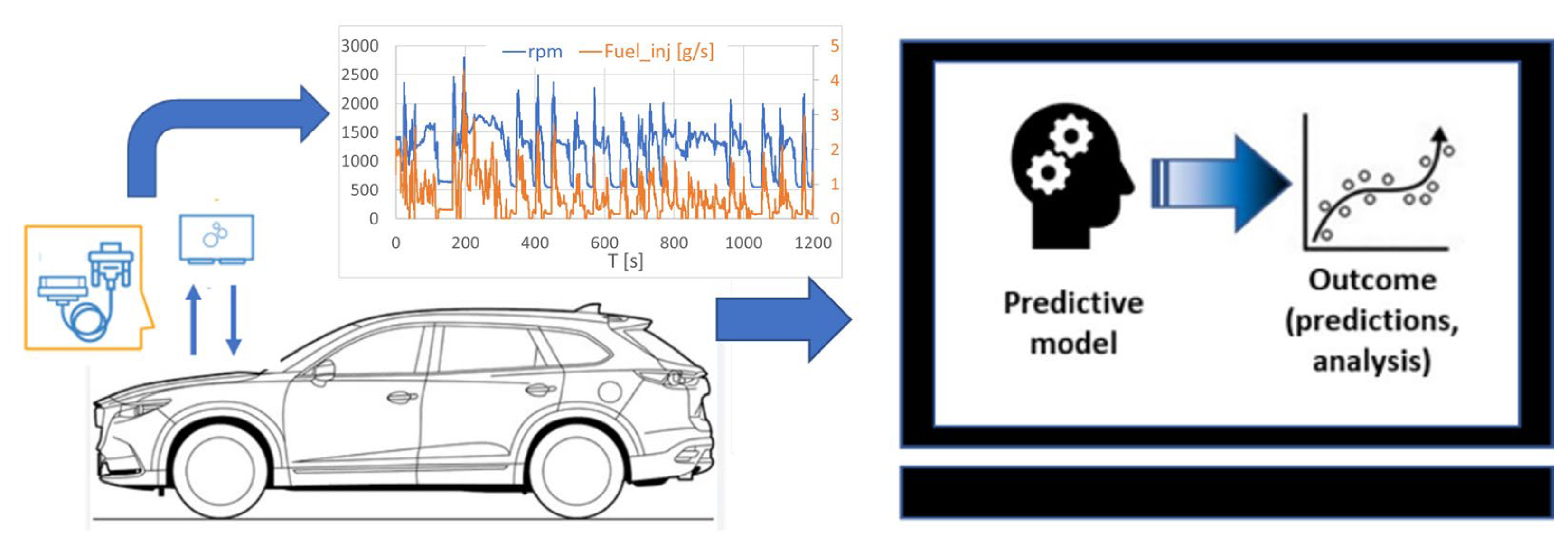
• Empirical data models: Such models are data driven, not physics based. Test data are used to create an abstract mapping of the system and to select the variables to be studied. A crescent field of investigation involves the use of Artificial Intelligence (AI). AI uses computer codes to perform cognitive functions, such as perceiving, reasoning, learning, and problem solving. It is used in, for example, robotics and autonomous vehicles, computer vision, language, virtual agents, and machine learning. AI machine learning involves the use of AI tools to analyze very large data sets. Machine-learning algorithms detect patterns and learn how to make predictions and recommendations by processing data and experiences. In this way, a machine learning model can be considered a digital twin: a nonphysical model that has been designed to accurately reflect an artificial or physical system, wherein sensors are placed to acquire a variety of data about the system performance (see Figure 1).

Transient vehicle tests generate a huge amount of data, making them a potential subject for analysis using machine learning tools. In an author’s previous publication [22], data from fuel consumption transient vehicle tests carried out at the Argonne National lab were analyzed using both semi-empirical and machine learning models to predict the influence of lower viscosity oils on fuel consumption. The machine learning model was “trained” using only the cold test phase results, and it was able to predict with good accuracy the fuel consumption in the hot phase cycle, when the oil temperature is higher and consequently the oil viscosity is lower.

Various types of machine learning algorithms exist, such as supervised, unsupervised, semi-supervised, and reinforcement learning algorithms. The literature on these and the tools they use are abundant and constantly updated. A recent overview can be found in [23]. Machine learning models have been used to predict vehicle fuel consumption. For instance, Hien [24] made use of a multilinear regression model to predict the CO₂ emissions and fuel consumption of a light duty vehicle. Katreddi [25] predicted the fuel consumption of a heavy-duty engine using a Random Forest model, obtaining an error of 0.04% between the prediction and measurements. Gong et al. [26] trained a Random Forest model with 200 trees and obtained an R² of 0.86 and an error equal to 0.15%.

Although more complex and CPU intensive, Artificial Neural Network (ANN) models tend to have better performance than other models. An ANN provides different configurations to train and improve model predictions. The variables that perform the neural network are the input data, the hidden layers, and the neurons per layer. He [27] used seven control parameters for the optimization of diesel engine emissions. The developed ANN predicted the cylinder temperature, cylinder wall heat transfer, cylinder pressure, NOx and soot emissions. Cruz-Peragon [28] used a combination of angular speed measurements and an ANN for combustion fault diagnosis. Ziolkowski [29] used an ANN with 12 input variables to predict the fuel consumption of passenger cars, obtaining an R² equal to 0.98. Perrota [30] trained an ANN with 12 input variables to predict the fuel consumption of trucks, obtaining an R² equal to 0.85. Du [31] trained 5 ANN for predicting fuel consumption with 8 input variables. Parlak [32] predicted the brake specific fuel consumption and exhaust temperature of a diesel engine, obtaining a maximum error equal to 0.02%.

Most of the mentioned references trained and tested the models using the same test data, with usually 75% of the data used for model training, and the other 25% used for assessing (“testing” in AI jargon) the model fitness. In the current work, two machine learning model types, the Random Forest and Artificial Neural Network types, were trained to predict instantaneous fuel consumption using just part or given emission tests, e.g., the FTP75 cold start. A machine learning digital twin was created and then used to predict instantaneous fuel consumption for different transient emission tests not used during the model development. The models were optimized regarding their input variables and number of trees or neurons per layer. The model accuracy was evaluated using different engine parameters and sub-data sets. The risk of trusting “only” the statistical values, such as the model’s R² value and the error between the model and reality, is discussed.

2. Methodology

2.1. Vehicle Characteristics

ECU or OBD data from three vehicles were used to investigate the use of AI models in transient tests (see

Table 1. Tested vehicle characteristics.

N3 Class Truck 18-Ton Euro 6	SUV * 2016 Mazda CX-9	Light Truck * 2017 Ford F-150
7.0-L, I6	2.5 L I4	3.5 L, V6
CI, TDI	SI TDI	SI, PFI and DI
210 kW	186 kW	280 kW
1150 Nm	420 Nm	637 Nm
9-speed manual	6-speed automatic	10-speed automatic

* Test data from the Downloadable Dynamometer Database [28] from the Advanced Mobility Technology Laboratory (AMTL) at Argonne National Laboratory under the funding and guidance of the U.S. Department of Energy (DOE) [33].

).

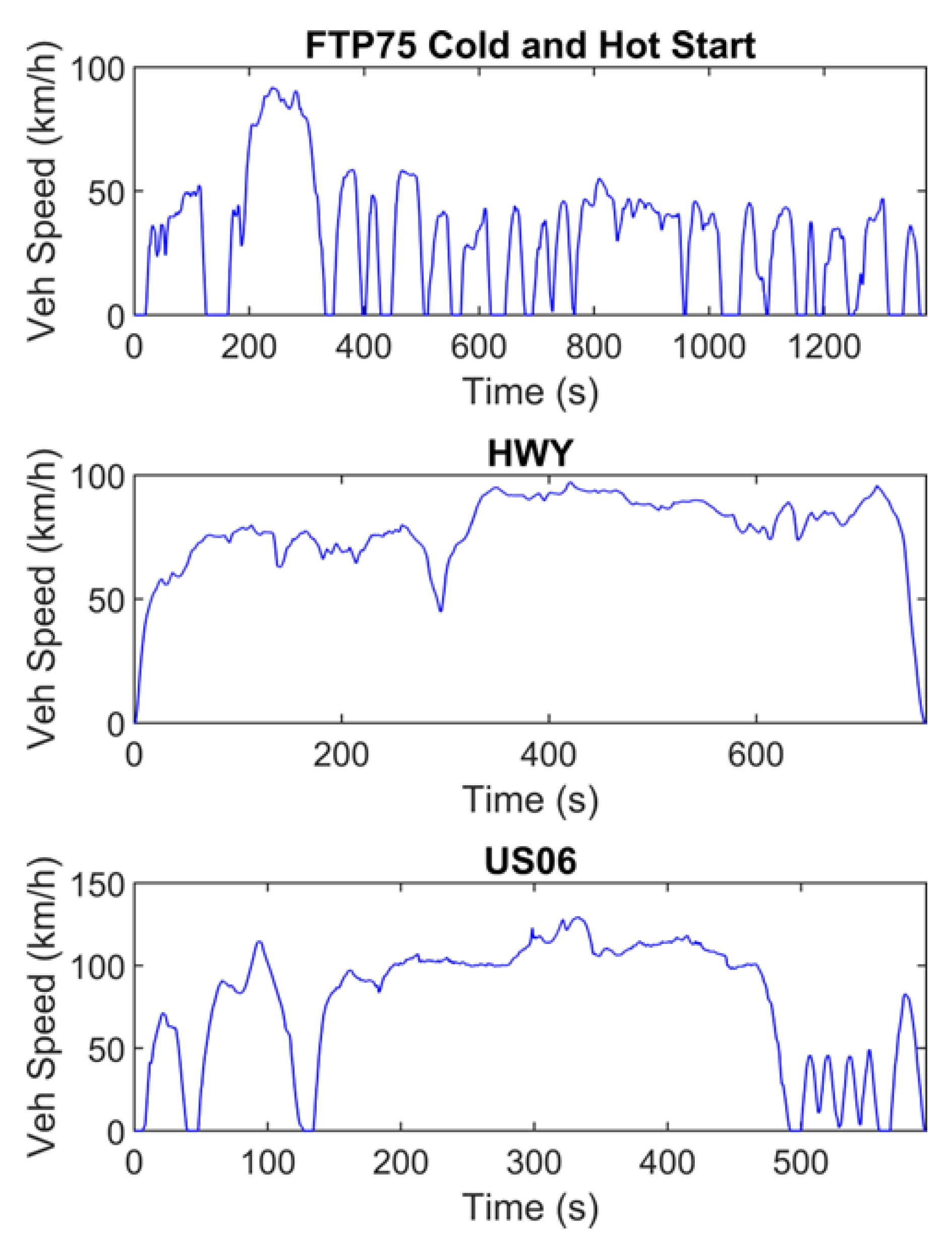
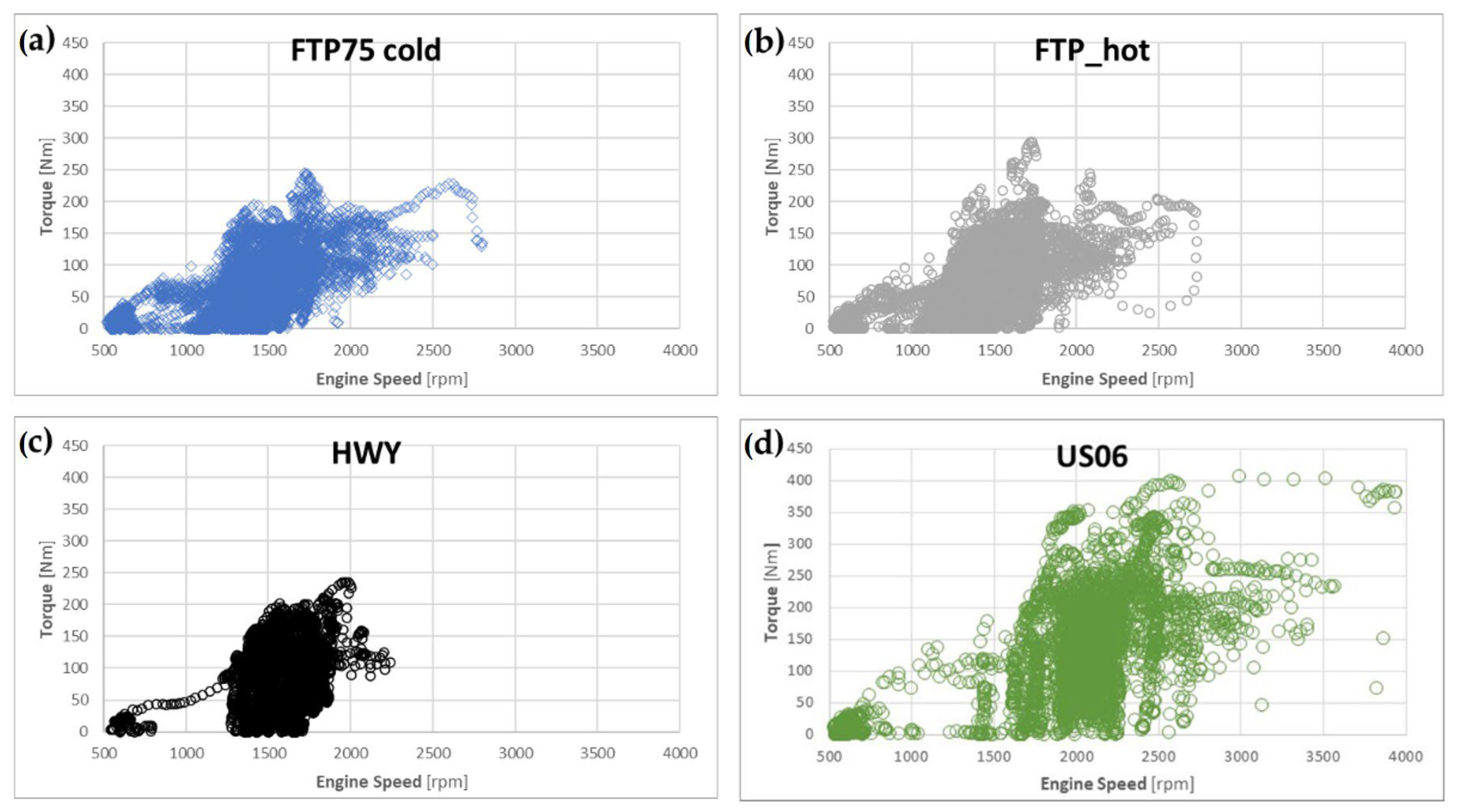
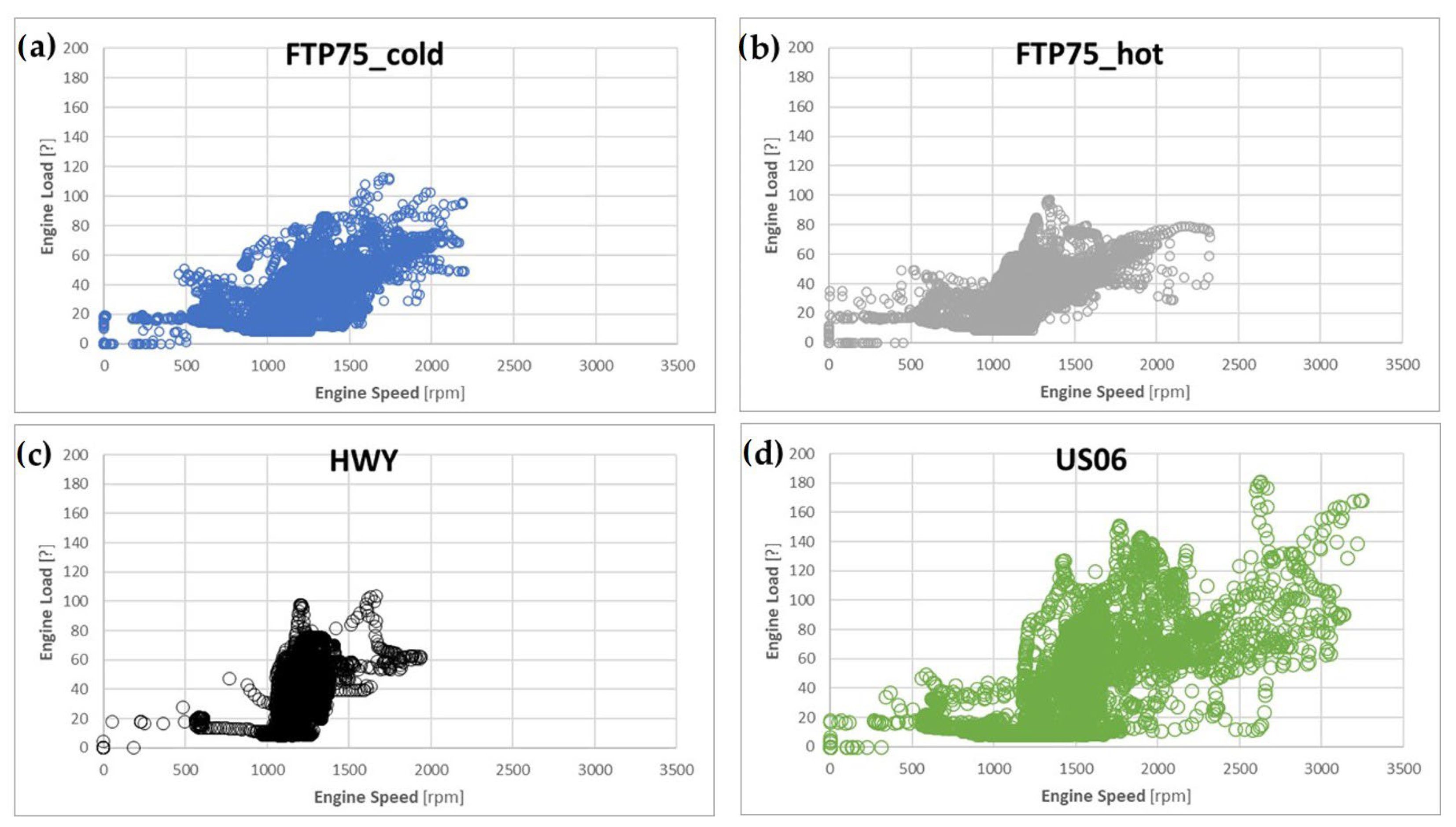
2.2. Cycle Characteristics

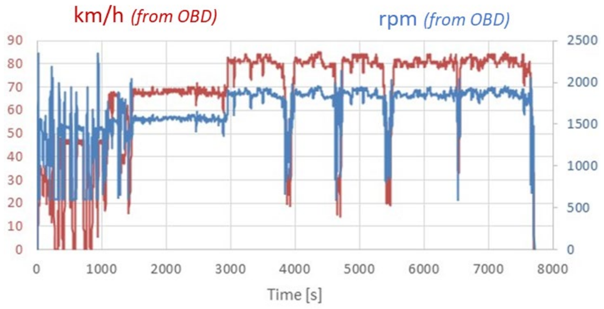
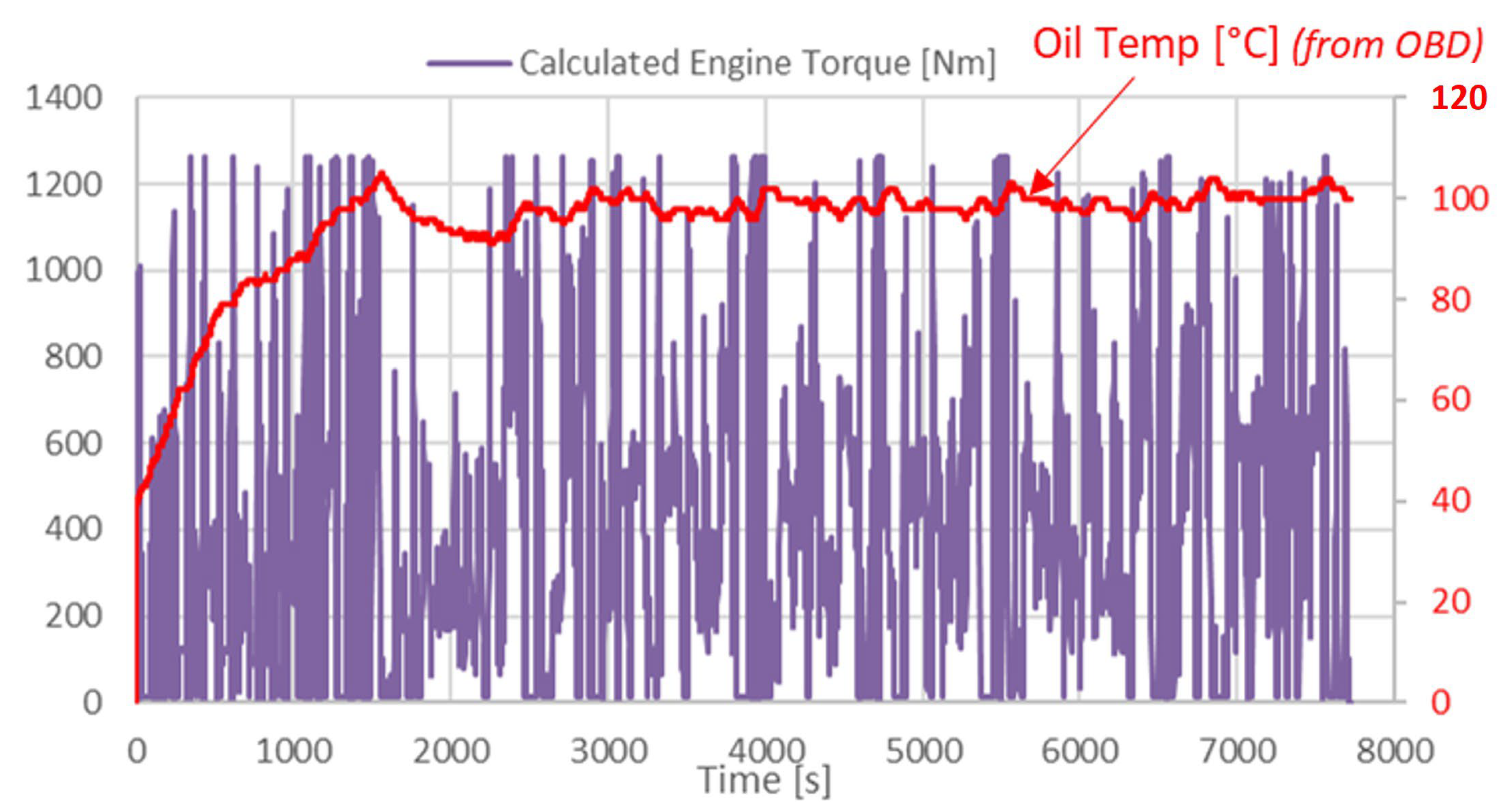
RDE Truck Test

The test conformed to the Brazilian RDE (Real Drive Emissions) specifications, with a 143 km length and time ratios of 14% acceleration, 13% deceleration, 71% cruising and 2% stop. Figure 2 and Figure 3 show various truck OBD readings during the RDE test.

For the SUV and light truck, data from 4 emission tests from the ANL laboratory [33] were used: FTP75 cold and hot start, Highway cycle and US06 cycles. Figure 4 shows the mandatory vehicle speed profile for each cycle, and

Table 2. Emission cycle characteristics.

	FTP75	Highway	US06
	Stop and Go Urban Traffic	Free-Flow Traffic at Highway Speeds	Higher Speed, Harder Acceleration & Braking
Engine startup	Cold and warm	Warm	Warm
Top speed (km/h)	90	97	129
Average Speed (km/h)	34	77.7	77.9
Max. accel. (m/s2)	1.47	1.43	3.78
Distance	17.7	16.6	8
Time (min)	23	12.73	12.9
Stops	23	None	4
Idling time (%)	18	None	7

shows the main cycle characteristics.

To comply with the mandatory speed profile, different vehicles will demand different engine rpm/torque combinations. Figure 5 and Figure 6 show the engine usage maps for the SUV and the light truck during the different transient cycles. For the light truck, engine load is referenced as the quantity of air in the cylinder. The nominal displacement volume is represented by 100%, while values higher than 100% indicate boosting. Notice that although the FTP75 cold and hot start cycles had the same vehicle speed profile, they demanded a different engine usage. Notice also that the Highway cycle and especially the US06 cycle demanded higher rpms and loads from the engine.

2.3. Machine Learning Models

All modern vehicles have an ECU (or OBD) reading and controlling engine parameters. Using a simple datalogger, detailed and instantaneous readings can be carried out in real time at a much lower cost than engine or car dynamometer tests. Figure 7 shows a scheme of using ECU reading and machine learning models to predict, e.g., instantaneous fuel consumption for different cycles, engine calibrations and even oils with different viscosities by imposing a different oil temperature to match the oil viscosity to be studied (see example in [16]).

In transient tests, it is common for more than one hundred variables to be read. These variables are obtained from external vehicle instrumentation and from the engine control unit (ECU). Most of the variables are not related to vehicle fuel consumption and can lead to a machine learning model receiving poor training. The following variables were chosen, a priori, for most of investigations ahead: vehicle speed and acceleration, engine rpm, torque, and oil temperature.

Two different supervised machine learning models were used to predict the instantaneous fuel consumption during the cycles. As usual for machine learning, the two models were only trained with a random subset of 75% of data. For the car and light truck, model was trained and validated with the FTP 75 Cold phase, and then the model was used to predict instantaneous fuel consumption for the other three transient cycles.

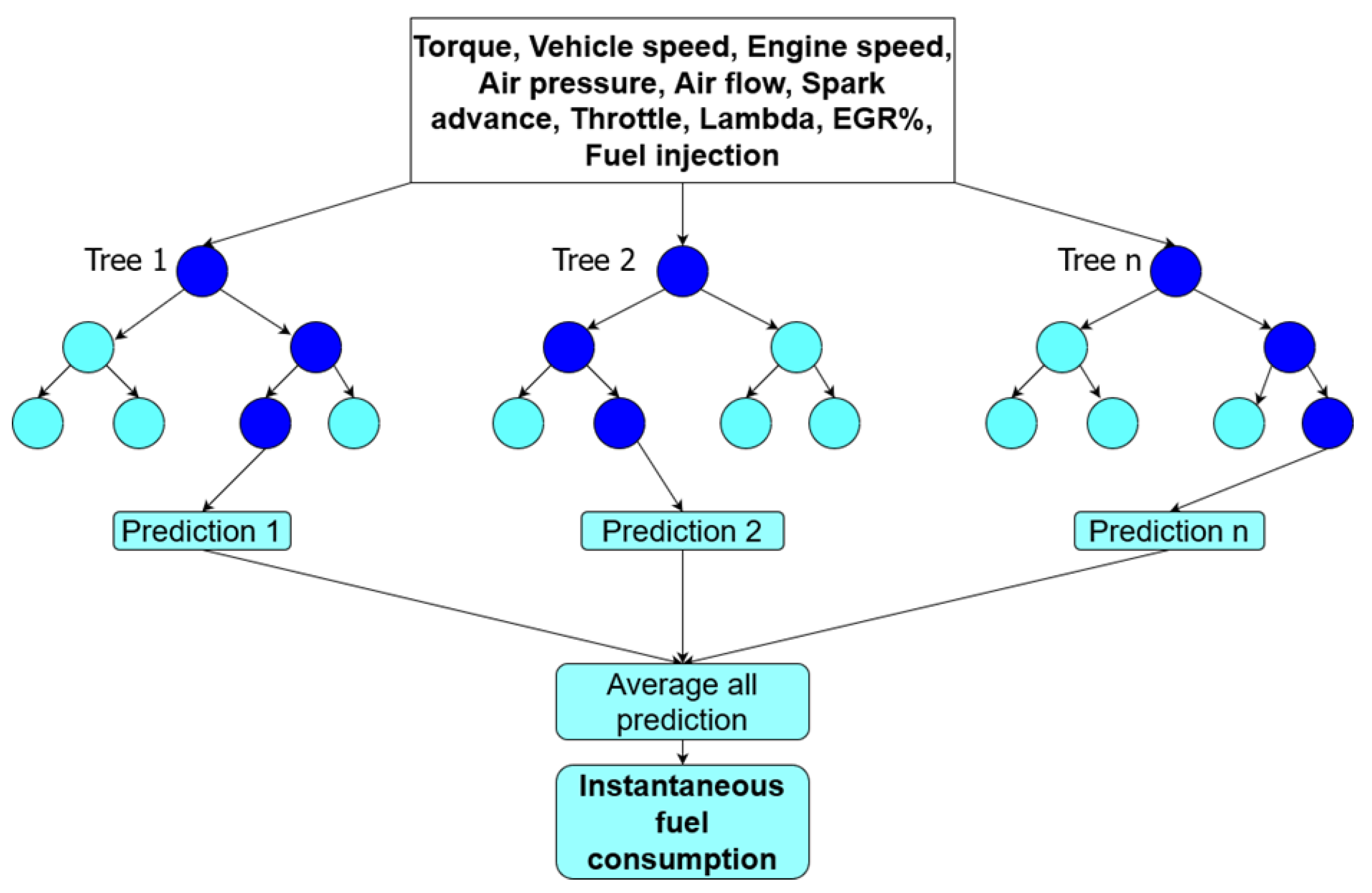
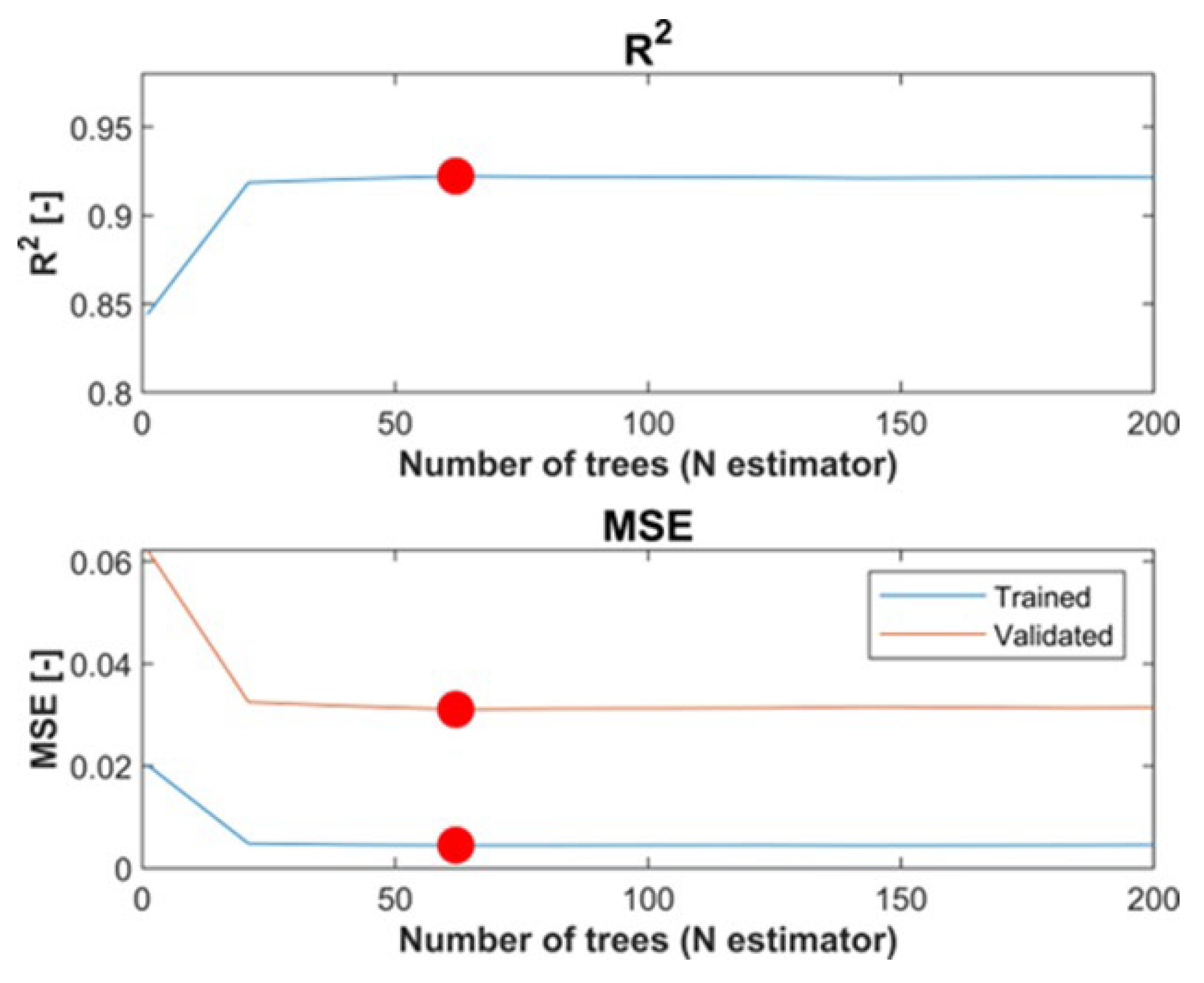
• Random Forest: The Random Forest method uses bootstrapping to create subsets of the original dataset containing a random portion of all the elements. The method involves a combination of multiple tree predictors (see Figure 8) that aggregates the results, casting the most popular outcome and thus reducing variation compared to normal decision trees. To find the threshold that best separates the data, random subsets of features are used. Many trees will be trained in a weaker way and each of them will produce a different prediction. However, these weaker predictions tend to cancel out each other, and the stronger predictions tend to dominate. For regression tasks, the mean or average prediction of the individual trees is used [34].

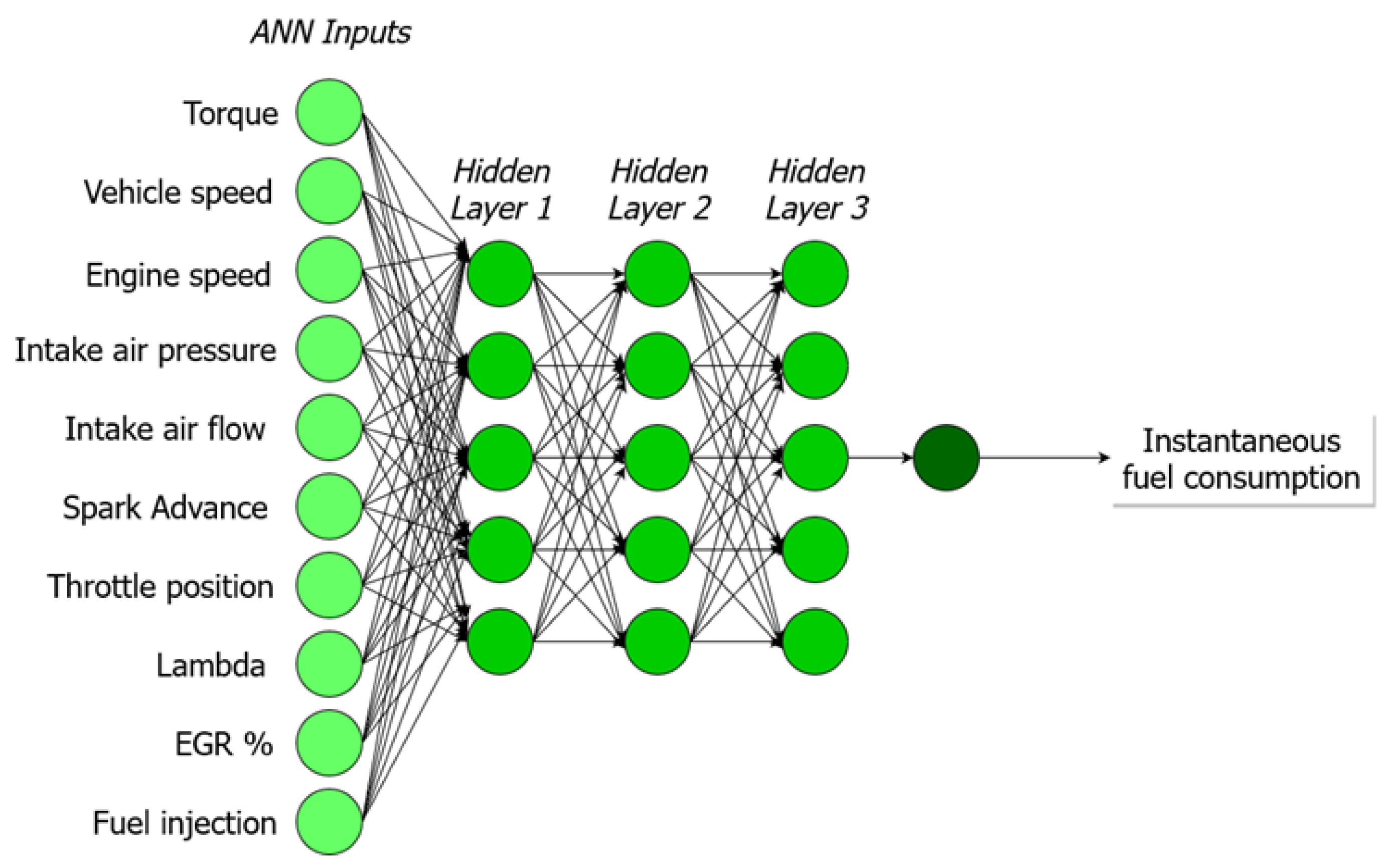
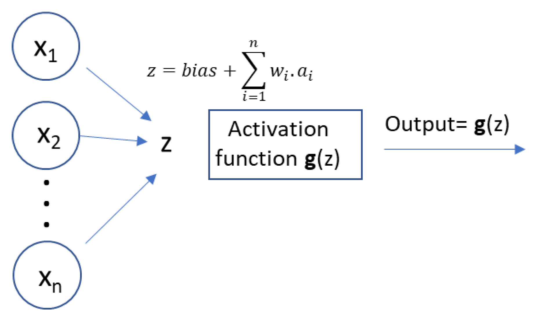
• Artificial Neural Network: An ANN is a group of interconnected artificial neurons interacting with one another in a concerted manner, loosely reproducing the interaction of neurons in a biological brain (see Figure 9). Each artificial neuron has several inputs and produces a single output which can be sent to multiple other neurons, meaning it exhibits a high degree of connectivity, which is also called multilayer perceptrons. In this work, multilayer perceptrons with 3 hidden layers and up to 20 neurons per layer were trained to predict the instantaneous fuel consumption of a given vehicle during the vehicle test cycle. Hidden layer selection has been used by other authors to predict fuel consumption in light-duty vehicles [35,36,37,38,39,40]. In the present study, the backpropagation (BP) method was used to train the neural network. This is common practice of fine-tuning the weights of a neural net based on the error rate obtained in previous epoch (iteration). Proper tuning of the weights ensures lower error rates, making the model reliable by increasing its generalization.

• R²: R-squared value is used to measure the goodness of fit or best-fit line. The higher R², the better the regression model, as most of the variation in actual values from the mean value is explained by the regression model.
• Mean Squared Error (MSE): Measures the average squared error of the model predictions. For each data point, the squared difference between the predictions and the target is calculated and used for the averages. The lower the MSE, the better the model. MSE is calculated as:

$$MSE=\frac{1}{N} {\displaystyle \sum }_{i=1}^N{(y_i-\widehat{y_i})}^2$$

(1)

Accumulated error in the cycle (∆%): in the cases discussed in this work, ∆% is the percentage difference between the model prediction for fuel consumption and the actual fuel consumption.

3. Results

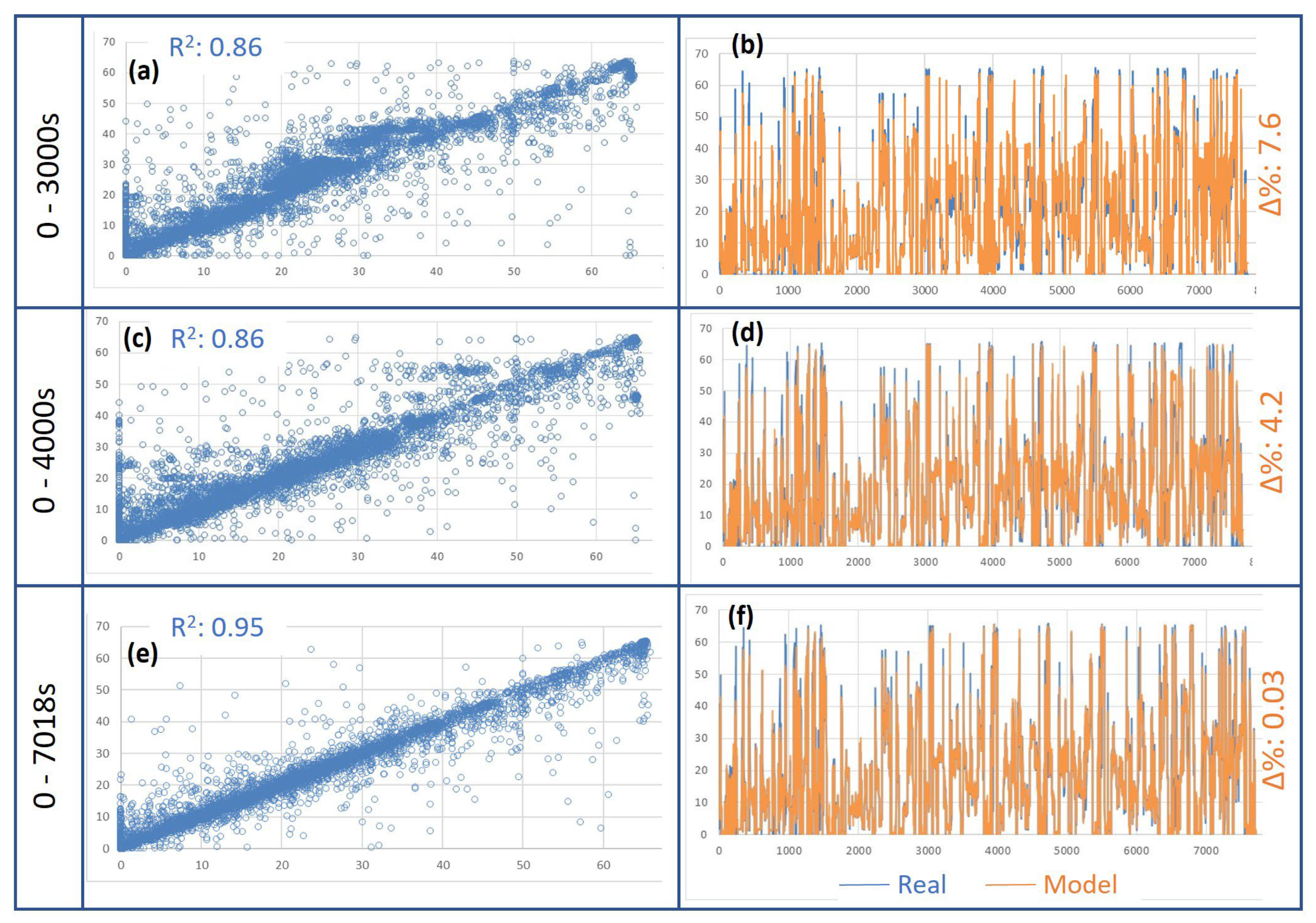
3.1. Truck RDE

Figure 10 shows the Pearson correlation values for the OBD variables obtained during the RDE test. As expected, engine torque was the variable with the highest influence on the fuel rate. The ECU oil temperature was read in the main oil gallery. Notice that truck acceleration, calculated from the truck speed, had the second highest influence on the fuel rate.

Three data sets, 0–3000 s, 0–4000 s and the complete RDE test, were used to investigate the developed Random Forest model’s ability to predict fuel consumption. Figure 11 and Figure 12 show the results when 75% of the complete RDE test was used for training. The error for the accumulated fuel consumption during the test, ∆%, was only −0.69%.

Figure 13 illustrates the impact of the datasets used for model training/validation. When using only the 0–3000 s, and when the truck had not yet reached the highway, the model’s performance was relatively poor. Even though the model was able to predict the instantaneous fuel rate trends and the R² was 0.86, the error, ∆%, was 7.6% for the accumulated fuel during the cycle. When using 0–4000 s, which included one of the four periods of the highway journey, the R² was almost unchanged, but the ∆% was reduced to 4.2. When using the complete RDE test (i.e., always 75% random data of the test) to train the model, the R² reached 0.95 and the ∆% was only 0.03.

Figure 14 illustrates the impact of the variables chosen to train the Random Forest model for the truck RDE test:

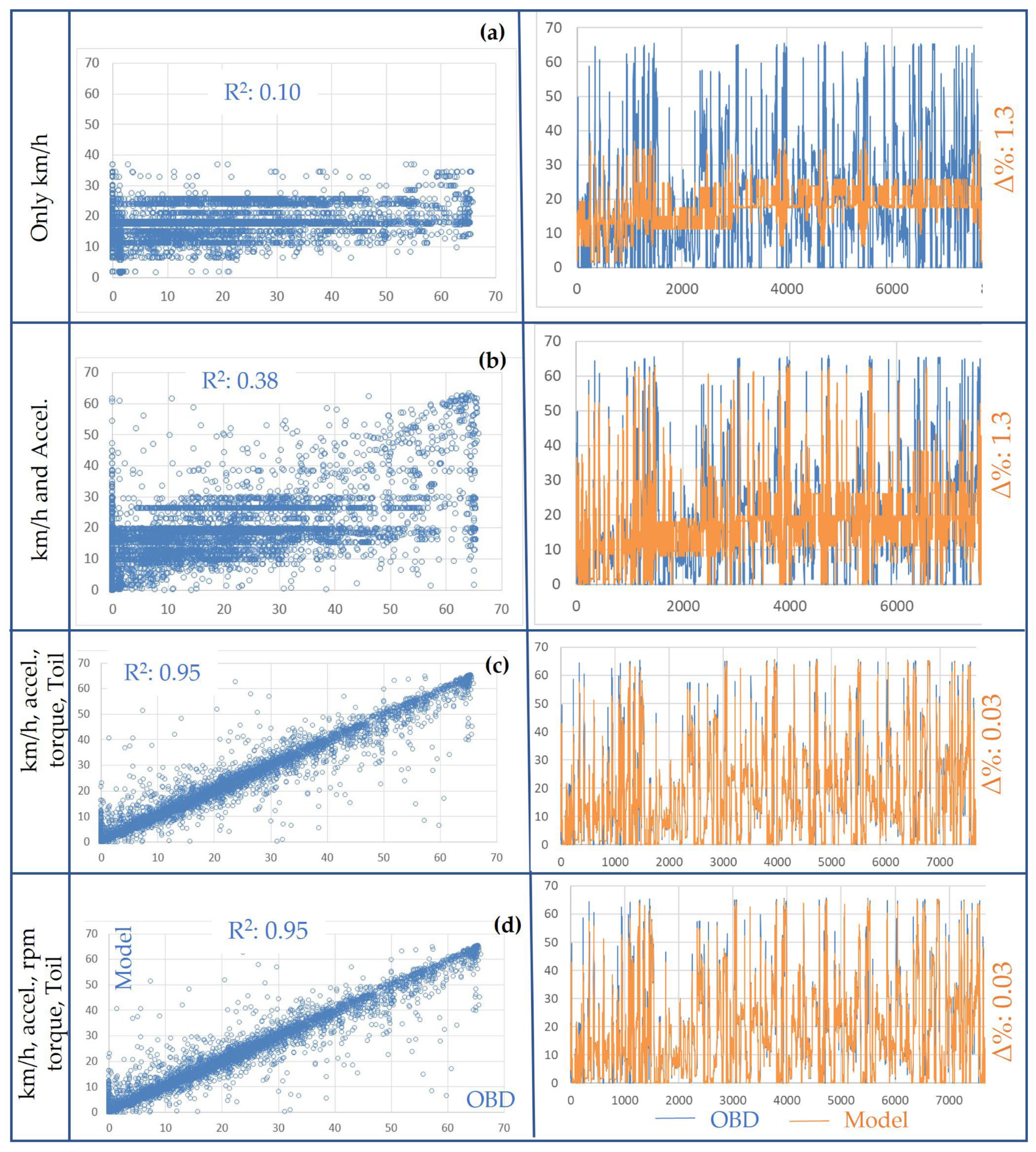
• For only the truck speed, the model’s performance was, of course, very poor. The R² was 0.06 but the accumulated cycle error for the fuel consumption, ∆%, was only +1.3%. One should be careful when analyzing the model’s performance. The total error was (almost by chance) very low, but the model very poorly represented the actual truck, as indicated by Figure 14a.
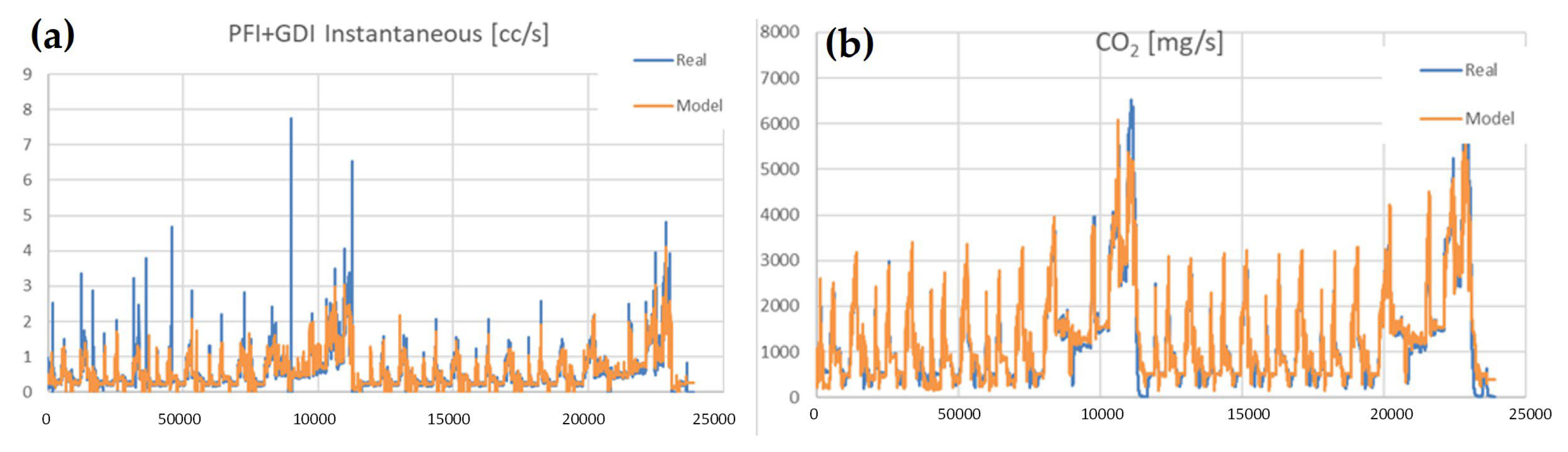
• When including the truck acceleration, calculated from the OBD truck speed, the model’s performance increased significantly. The R² remained low, but the spiky fuel rate was reproduced relatively well by the model. See Figure 14b.
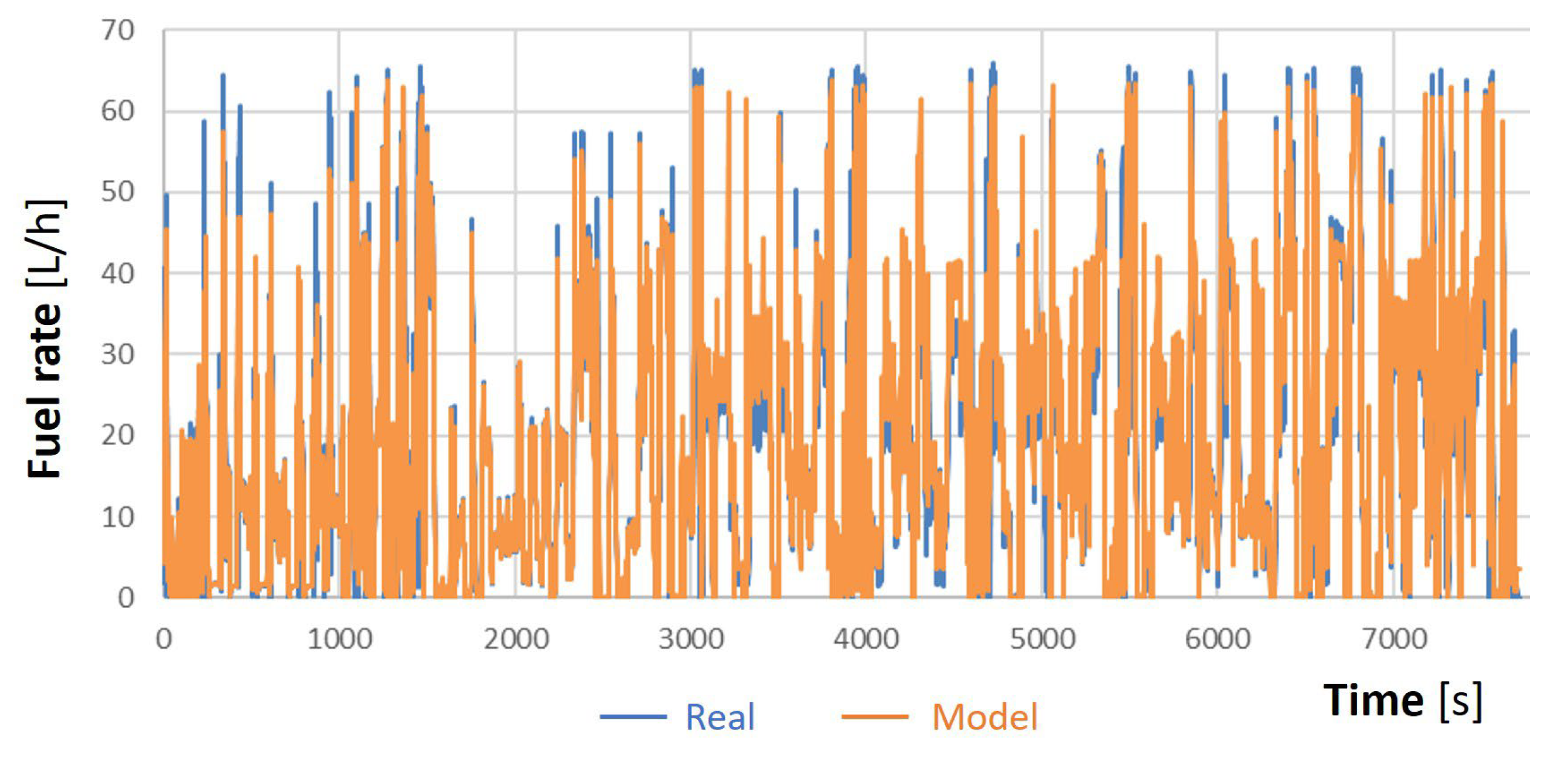
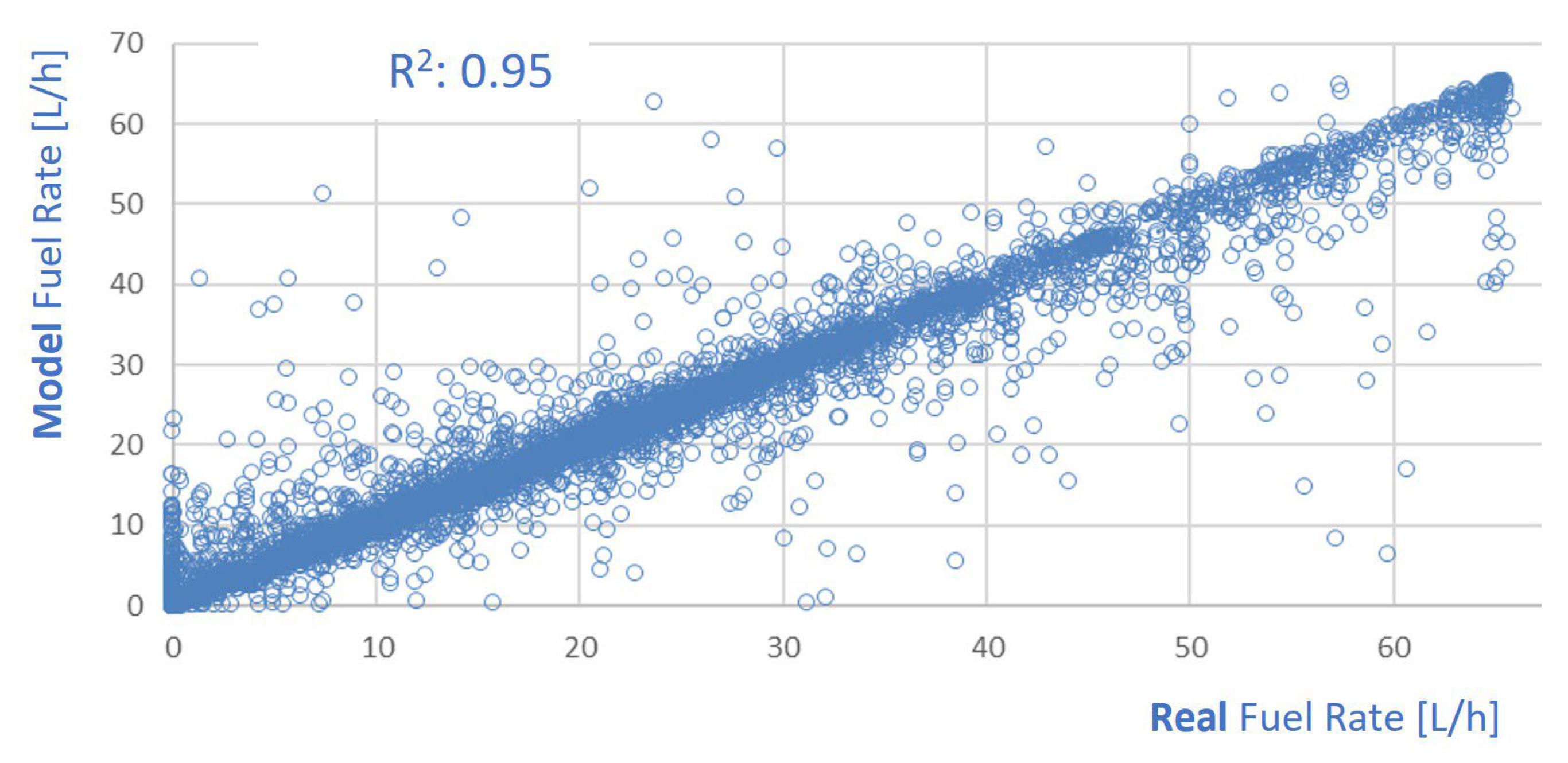
• When including the engine torque and oil temperature, the model’s performance was very good. The R² increased to 0.95 and the ∆% was only 0.03. See Figure 14c.
• Due to the low variation in the engine rpm during the test, including the rpm led to almost no difference in the model’s performance. See Figure 14d.

3.2. SUV

In the ANL database, both instantaneous dynamometer measurements and ECU readings are available. The measured fuel consumption and ECU fuel rate correlated quite well, as expected. Figure 15 compares the dynamometer equipment measurements with the ECU readings after bringing the latter to the same unit. For the original 0.1 s time acquisition, there were some deviations between the ECU readings and dynamometer measurements. Such deviations almost disappeared when the values were averaged to a 1.0 s data rate.

To demonstrate the model’s ability when using only ECU data, the ECU variables listed in Figure 16 were analyzed. The oil temperature was externally measured by a sensor installed in the oil dipstick.

The variables selected to train the model were as follows:

• From the external vehicle instrumentation: The fuel consumption with the mass flow meter (target variable), engine coolant temperature and engine oil temperature.
• From the Engine Control Unit (ECU): the engine torque, vehicle speed, engine speed, intake air pressure, air flow, spark advance, throttle, EGR percentage and lambda.

These variables were selected as, a priori, they were considered to potentially have a large impact on engine fuel consumption. However, as mentioned earlier, some variables may be more or less influential depending on the cycle characteristics. Figure 17 shows the correlation factors for the instantaneous fuel consumption. Figure 18 shows the interdependency of the different parameters. Some important comments can be made here, which serve to both illustrate which engine parameters were more influential in each cycle as well as highlight the machine learning models’ development:

−

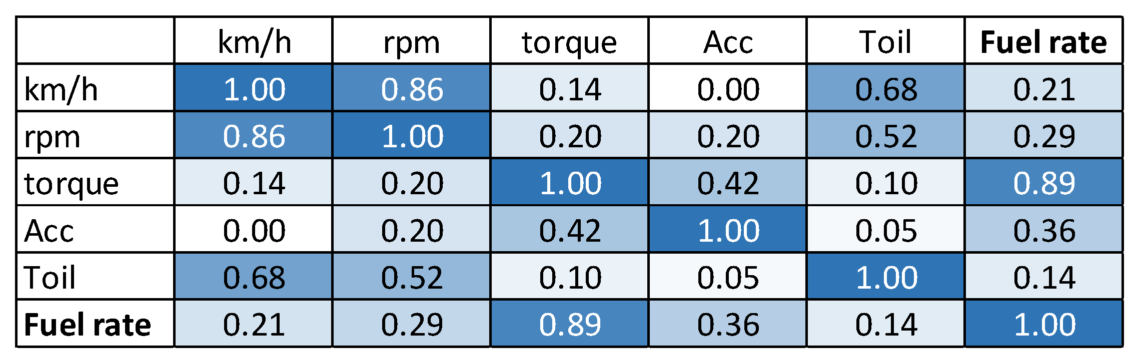
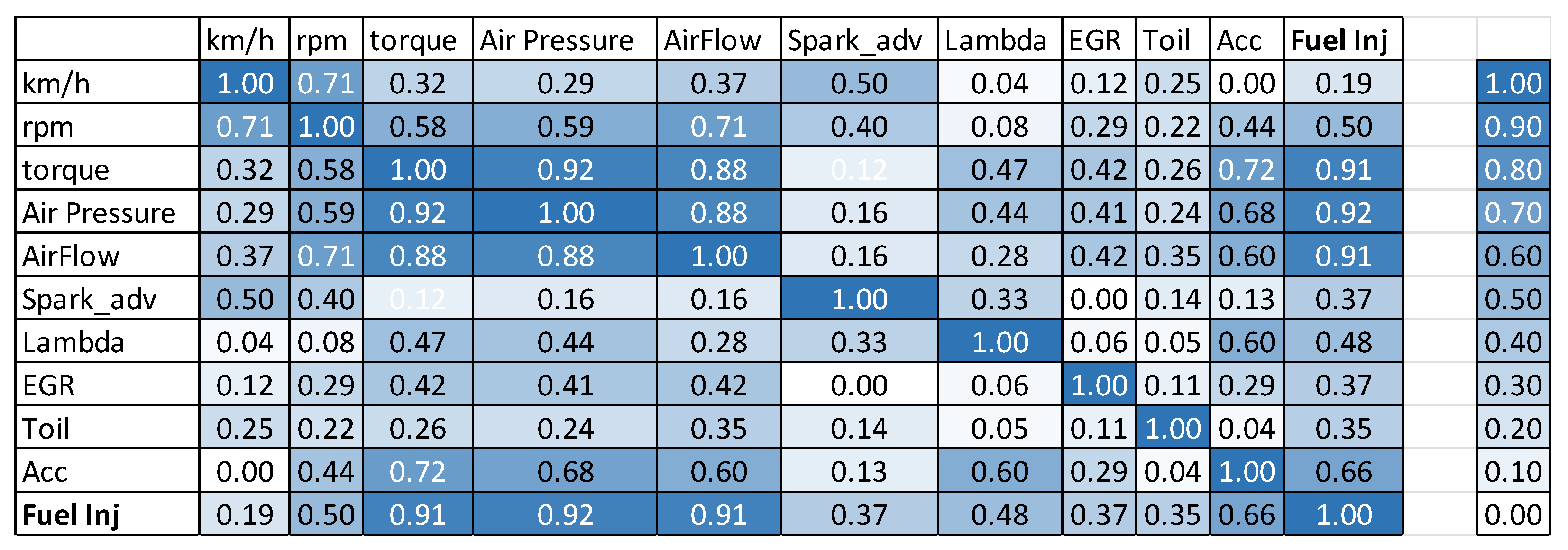
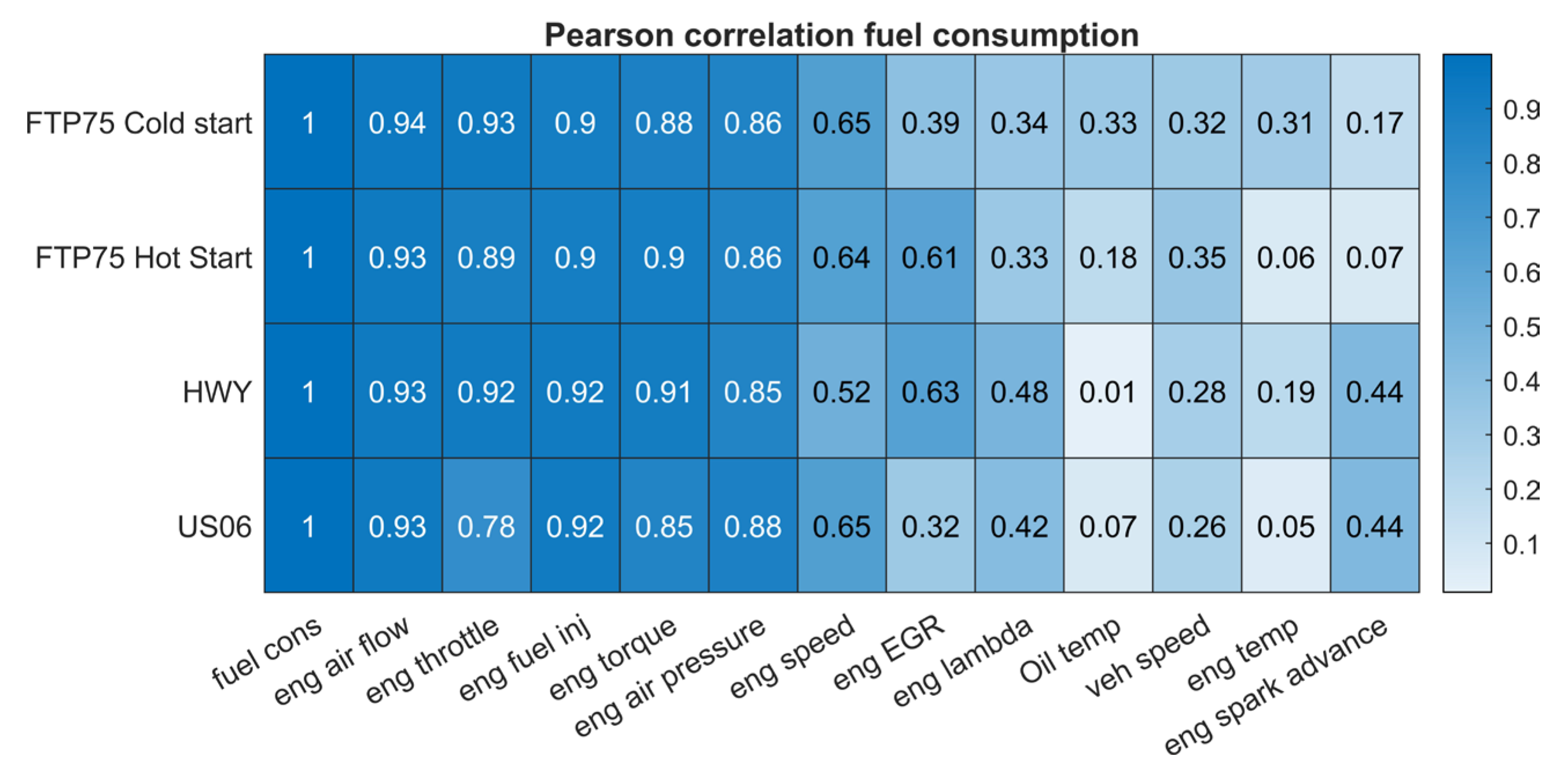
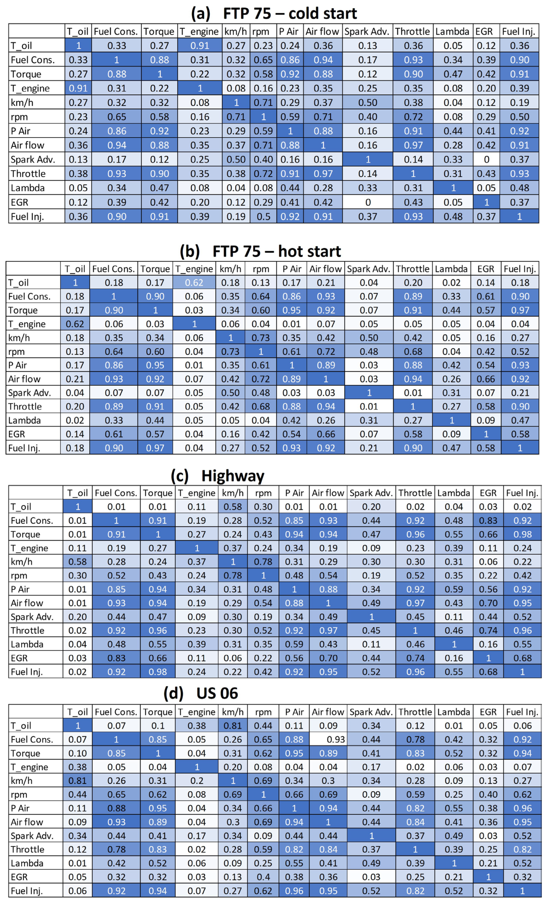
The air flow, air pressure and engine torque were obviously the major influences on the instantaneous fuel consumption.

−

Some correlated parameters, such as the engine air pressure and air flow, were probably able to be omitted, with only engine torque needing to be used instead.

−

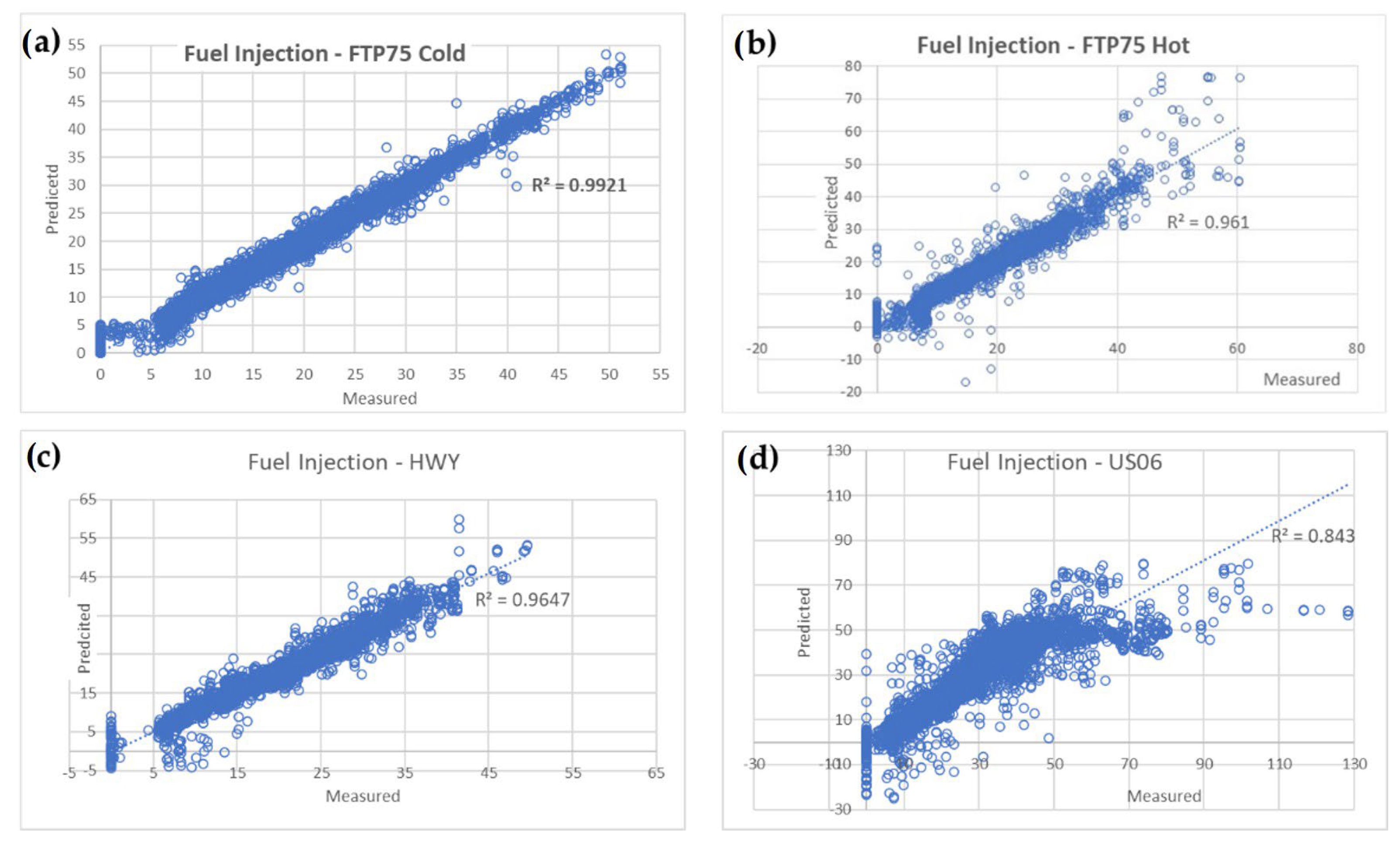
While the oil temperature had a relatively high influence in the FTP75 cold and hot start cycles, its influence was negligible in the highway and US06 cycles, in which the engine was already hot and the engine loading was much more severe.

−

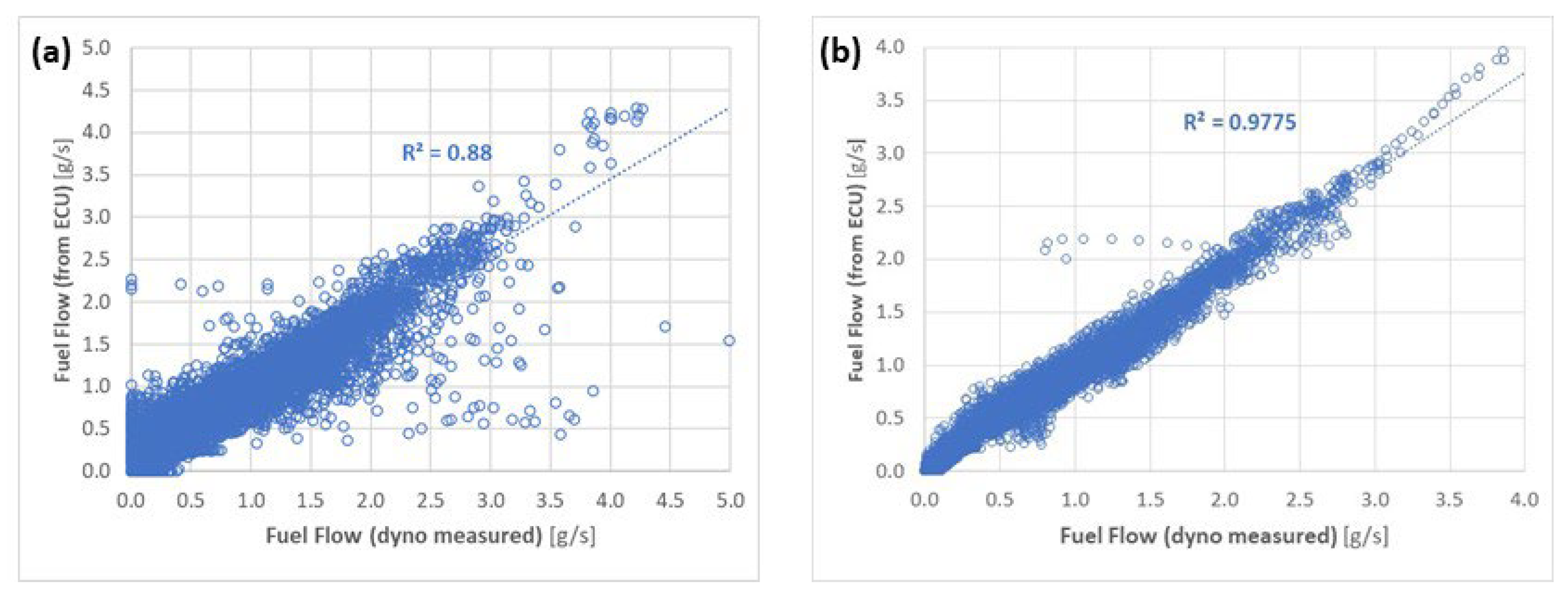
The fuel injection, read from the ECU, obviously correlated well with the measured fuel consumption. As mentioned earlier, this creates the opportunity to use only the vehicle ECU data (or the truck/bus OBD data) instead of much more expensive dynamometer or specific measurement equipment. This will be explored further in Section 3.4.

Table 3. Results for SUV—FTP75 cold start.

	Training		Overall Cycle
	R2	MSE	R2	MSE
Random Forest	0.92	0.004	0.97	0.011
ANN	0.95	0.041	0.95	0.042

shows the fitness of the two machine learning models during their training and the overall cycle in which they were trained (FTP75 Cold start) after model optimization. The Random Forest model recorded a higher R² value but also a higher MSE. Most of the values fitted well with the measurements but with a little higher deviation than the trained set.

Table 4. Fuel consumption of SUV.

	Measured [g]	Model Error [%]
		Random Forest	ANN
Cold Start	832.9	0.1	0.1
Hot Start	745.3	1.4	0.7
HWY	750.4	2.4	−0.2
US06	995.7	−7.9	−0.2

shows the fuel consumption predictions for each cycle and for the two machine learning models.

In the training cycle (FTP75 cold start), the Random Forest model was the best fitting model for estimating the instantaneous fuel consumption. However, it recorded worse predictions for the other considered cycles, obtaining, for instance, an error of almost 8% for the US06 cycle. The reasons for this behavior include the fact that there were different engine operating points in each test cycle. The Random Forest model is less flexible when the values used are not those used for training. While the HWY operating points were in the same engine map region of the cycle used for model training (FTP75), during the more aggressive US06 cycle, the engine reached higher power than that covered in the model training (see Figure 6).

Figure 19 and Figure 20 compare the ANN predictions with the actual measurements for the instantaneous fuel consumption of the SUV. The instantaneous behavior was well predicted, with the model only failing in the very abrupt peaks.

3.3. Light Truck

The results for the light truck presented similar trends to those for the SUV, but the model errors were higher.

Table 5. Fuel consumption of light truck.

	Measured [g]	Model Error [%]
		Random Forest	ANN
Cold Start	1019.5	0.25	−0.08
Hot Start	924.8	6.50	−1.21
HWY	881.0	−0.20	−1.78
US06	1194.4	−10.4	−1.56

shows the model predictions and actual measurements for the four cycles.

3.4. Using Only ECU Data for the Light Truck Test

Figure 21 shows the ANN model results when it was trained with the ECU fuel rate data and, as earlier, when it used the FTP 75 cold start data. The model was then used to predict the instantaneous fuel rates for the other three cycles. The R² values were 0.99, 0.96 and 0.96 for the cold start, hot start, and highway cycles, respectively. All of these R² values were higher than those obtained when using the dynamometer fuel consumption measurements. Only the US06 showed a lower R² value of 0.84, which was still very similar to the R² value of 0.85 obtained when using the dynamometer fuel consumption measurements.

4. Discussion

In this study, the machine learning models used were able, with reasonable accuracy, to predict instantaneous fuel consumption during different vehicle cycles. The engine map of the training data needed to cover the ones used for prediction. For example, using the US06 cycle as the training data for the other three cycles significantly decreased the model accuracy. For the SUV, the R² drastically reduced from 0.89 to 0.20 and from 0.88 to 0.56 for the FTP75 cold and hot start cycles, respectively.

Transient cycles produce a huge amount of measurement data. Fuel consumption, as well as other performance criteria, is affected differently by various engine parameters, such as oil temperature, EGR%, spark timing, etc. A simple plot of the correlation factors, as shown in Figure 10 and Figure 16, Figure 17 and Figure 18, can indicate the parameters that are more influential in the different cycles and regarding the optimization goals.

Some of the predictions carried out measured several parameters (the engine lambda, EGR%, etc.). Information on these parameters was available in the measured data. In more realistic cases, fewer instantaneous parameters would probably be available. Regardless, the proposed AI method can be used to carry out much cheaper studies, especially those using transient cycles with huge amounts of data, as demonstrated in Section 3.1 and Section 3.4.

Further, the number of trees and neurons in the Random Forest and ANN digital twins methods, respectively, was optimized. This optimization was applied in addition to the intrinsic model training, in which each tree or neuron was “optimized”. For the Random Forest method, the intrinsic optimization process occurs in each tree after it receives a subset of the training data. In each node, the dataset is divided in two and a threshold value is obtained by minimizing the sum of squared residuals. The process of creating nodes continues until a “leaf node” is reached and a prediction value is obtained; this can occur for different reasons, but the simplest is because the minimum number of observations has been hit. For the ANN method, the optimization process uses gradient descent via backpropagation to define the value for each weight, wi, bias and activation transfer to achieve the “best” model performance. See Figure 22 for more details.

4.1. Optimizing Number of Trees in Random Forest

Theoretically, the number of decision trees in a Random Forest model can range from one up to infinity. The higher the number of decision trees, the higher the precision of the model. However, a high number of decision trees can cause high CPU consumption, so in this study, the model was optimized. The model was trained using 1 to 1000 decision trees. After this, the R² coefficient and MSE training and validation values were used to select the optimum number of trees. It was found that for the studied cases, 50 trees already produced a good prediction. See Figure 23 for more details.

After the training and validation with the FTP75 cold cycle was carried out, the number of trees with a good balance between the prediction error and CPU time was found to be 62 and 41 for the SUV and light truck, respectively. Using a higher number of trees did not increase the fit of the model and increased the CPU time.

Table 6. Model indicators for the cold start cycle used for training.

	SUV	Light Truck
Number of Trees	62	41
R2	0.92	0.88
MSE training	0.004	0.003
MSE validation	0.031	0.075

shows the model indicators.

4.2. Optimizing Number of Neurons in the ANN Model

Three hidden layers were chosen for predicting the fuel consumption during each vehicle test cycle. Each hidden layer had a maximum of 20 neurons. The criterion to select the number of neurons per hidden layer was that the maximum difference between the measured and predicted fuel consumption in the cycle should be 1.5%. A total of 15 combinations accomplished that criterion. With those combinations, the neural network selected was that which had the lowest average absolute error in predicting the fuel consumption. See

Table 7. Different combinations of hidden neurons per layer for the SUV.

Hidden Neurons			Accumulated Pred. vs. Measured [%]				Avg Absolute Error [%]
Layer 1	Layer 2	Layer 3	Cold Start	Hot Start	HWY	US06
1	1	2	0.10	0.76	−0.82	−0.89	0.65
	2	7	0.08	0.66	−0.15	−0.19	0.27
	3	11	−0.02	0.48	−0.72	−0.63	0.46
	14	1	0.10	0.75	−0.87	−0.89	0.65
2	1	6	−0.59	−0.03	0.57	0.03	0.31
		11	−0.12	0.33	−0.43	−0.90	0.44
	4	18	0.05	0.72	−0.78	−0.53	0.52
	8	19	0.19	0.66	−0.35	−0.43	0.40
	13	9	−0.22	0.33	−0.76	−0.53	0.46
	5	2	−0.08	0.71	0.19	−0.49	0.37
	7	2	−0.14	0.72	−0.18	−0.20	0.31
7	2	6	0.03	0.71	0.41	−0.59	0.43
	9	11	−0.29	−0.02	0.76	−0.11	0.30
15	15	7	−0.90	−0.51	0.58	−0.41	0.60
19	10		−0.07	−0.49	0.54	−0.91	0.50

.

For the SUV, the combination that fitted best with the criterion selected was the ANN with one, two and seven for the first, second and third neurons, respectively. See Table 6 for more details. For the light truck, the same approach led to a best combination with 5, 18 and 14 neurons, with an average absolute error of 1.2% obtained.

4.3. Future Work

The developed digital twins methods can be used to carry out much less costly vehicle tests and optimizations. As an example, the authors are currently using this method to predict fuel consumption and CO₂ emissions. See Figure 24 for more details.

5. Conclusions

• Modern vehicles have a myriad of sensors that are read in real time by the ECU/OBD. With the use of a datalogger, such data can be easily read and used by AI models, allowing for much cheaper tests and simulations.
• In this work, two machine learning models were trained and used to predict the fuel consumption of three vehicles during different transient cycles.
• The machine learning models were able to predict the instantaneous fuel consumption during transient emission cycles without needing to be programmed specifically for this problem.
• The variables chosen as input for training the models were key to achieving better model performance.
• The Artificial Neural Network model showed a better fit in predicting the fuel consumption for the four emission tests, being in all cases under the 2% error. However, compared with the simpler Random Forest model, the improvement in its model fitness came at a considerable expense regarding the CPU time. This amounted to a few minutes versus several hours for the Random Forest and ANN models, respectively.

References

- Tseregounis, S.; McMillan, M.; Olree, R. Engine Oil Effects on Fuel Economy in GM Vehicles—Separation of Viscosity and Friction Modifier Effects; SAE Technical Paper 982502; SAE: Warrendale, PA, USA, 1998. [Google Scholar]
- Bartz, W. Fuel Economy Improvement by Engine and Gear Oils. In Tribology for Energy Conservation; Elsevier: Amsterdam, The Netherlands, 1998; pp. 13–24. [Google Scholar]
- Hoshino, K.; Kawai, H.; Akiyama, K. Fuel Efficiency of SAE 5W-20 Friction Modified Engine Oil; SAE Technical Paper 982506; SAE: Warrendale, PA, USA, 1998. [Google Scholar]
- Taylor, R.I.; Coy, R.C. Improved fuel efficiency by lubricant design: A review. Proc. Inst. Mech. Eng. Part J J. Eng. Tribol. 2000, 214, 1–15. [Google Scholar] [CrossRef]
- Carvalho, M.; Seidl, P.; Belchior, C.; Sodre, J. Lubricant viscosity and viscosity improver additive effects on diesel fuel economy. Tribol. Int. 2010, 43, 12. [Google Scholar]
- Macián, V.; Tormos, B.; Ruíz, S.; Ramírez, L. Potential of low viscosity oils to reduce CO2 emissions and fuel consumption of urban buses fleets. Transp. Res. Part D Transp. Environ. 2015, 39, 76–88. [Google Scholar] [CrossRef]
- Dam, W.; Both, J.; Parsons, G. Taking Heavy Duty Diesel Engine Oil Performance to the Next Level, Part 1: Optimizing for Improved Fuel Economy; SAE Technical Paper 2014-01-2792; SAE: Warrendale, PA, USA, 2014. [Google Scholar]
- Carvalho, M.; Richard, K.; Goldmints, I.; Tomanik, E. Impact of Lubricant Viscosity and Additives on Engine Fuel Economy; SAE Technical Paper 2014-36-0507; SAE: Warrendale, PA, USA, 2014. [Google Scholar]
- Tormos, B.; Ramírez, L.; Johansson, J.; Björling, M.; Larsson, R. Fuel consumption and friction benefits of low viscosity engine oils for heavy duty applications. Tribol. Int. 2017, 110, 23–34. [Google Scholar] [CrossRef]
- Devlin, M.T. Common Properties of Lubricants that Affect Vehicle Fuel Efficiency: A North American Historical Perspective. Lubricants 2018, 6, 68. [Google Scholar] [CrossRef]
- Taylor, R.I.; Morgan, N.; Mainwaring, R.; Davenport, T. How Much Mixed/Boundary Friction is there in an Engine-and where is it? Proc. Inst. Mech. Eng. Part J J. Eng. Tribol. 2019, 234, 1563–1579. [Google Scholar] [CrossRef]
- Yamamoto, K.; Hiramatsu, T.; Hanamura, R.; Moriizumi, Y.; Heiden, S. The Study of Friction Modifiers to Improve Fuel Economy for WLTP with Low and Ultra-Low Viscosity Engine Oil; SAE Technical Papers 2019-01-2205; SAE: Warrendale, PA, USA, 2019. [Google Scholar]
- Tormos, B.; Pla, B.; Bastidas, S.; Ramírez, L.; Pérez, T. Fuel economy optimization from the interaction between engine oil and driving conditions. Tribol. Int. 2019, 138, 263–270. [Google Scholar] [CrossRef]
- Yoshida, S.; Yamamori, K.; Hirano, S.; Sagawa, T.; Okuda, S.; Miyoshi, T.; Yukimura, S. The Development of JASO GLV-1 Next Generation Low Viscosity Automotive Gasoline Engine Oils Specification; SAE Technical Paper 2020-01-1426; SAE: Warrendale, PA, USA, 2020. [Google Scholar]
- Tormos, B.; Jiménez, A.J.; Fang, T.; Mainwaring, R.; L-Garcia, E. Numerical Assessment of Tribological Performance of Different Low Viscosity Engine Oils in a 4-Stroke CI Light-Duty ICE; SAE Technical Papers (2022-01-0321); SAE: Warrendale, PA, USA, 2022. [Google Scholar]
- Tomanik, E.; Profito, F.J.; Tormos, B.; Jiménez, A.J.; Zhmud, B. Powertrain Friction Reduction by Synergistic Optimization of the Cylinder Bore Surface and Lubricant Part 1: Basic Modelling; SAE Technical Paper No. 2021-01-1214; SAE: Warrendale, PA, USA, 2021. [Google Scholar]
- Zhmud, B.; Tomanik, E.; Jiménez, A.J.; Profito, F.; Tormos, B. Powertrain Friction Reduction by Synergistic Optimization of Cylinder Bore Surface and Lubricant-Part 2: Engine Tribology Simulations and Tests; SAE Technical Paper No. 2021-01-1217; SAE: Warrendale, PA, USA, 2021. [Google Scholar]
- Zeman, J.; Papadimitriou, L.; Watanabe, K.; Kubo, M.; Kumagai, T. Model Ing and Optimization of Plug-In Hybrid Electric Vehicle Fuel Economy; SAE Technical Papers (2012-01-1018); SAE: Warrendale, PA, USA, 2012. [Google Scholar] [CrossRef]
- Lujan, J.; Climent, H.; Novella, R.; Rivas-Perea, M. Influence of a low pressure EGR loop on a gasoline turbocharged direct injection engine. Appl. Therm. Eng. 2015, 89, 432–443. [Google Scholar] [CrossRef]
- Li, Y.; Chen, H.; Tian, T. A Deterministic Model for Lubricant Transport within Complex Geometry under Sliding Contact and Its Application in the Interaction between the Oil Control Ring and Rough Liner in Internal Combustion Engines; SAE Technical Papers No. 2008-01-1615; SAE: Warrendale, PA, USA, 2008. [Google Scholar] [CrossRef]
- Tormos, B.; Martin, J.; Blanco-Cavero, D.; Jimenez-Reyes, A. One-Dimensional Modeling of Mechanical and Friction Losses Distribution in a Four-Stroke Internal Combustion Engine. J. Tribol. 2020, 142, 11703. [Google Scholar] [CrossRef]
- Tomanik, E.; Tomanik, V.V.; Morais, P. Use of Tribological and AI Models on Vehicle Emission Tests to Predict Fuel Savings through Lower Oil Viscosity; SAE Technical Paper (2021-36-0038); SAE: Warrendale, PA, USA, 2021. [Google Scholar]
- Sarker, I.H. Machine Learning: Algorithms, Real-World Applications and Research Directions. SN Comput. Sci. 2021, 2, 160. [Google Scholar] [CrossRef]
- Hien, N.L.H.; Kor, A.L. Analysis and prediction model of fuel consumption and carbon dioxide emissions of light-duty vehicles. Appl. Sci. 2022, 12, 803. [Google Scholar] [CrossRef]
- Katreddi, S.; Thiruvengadam, A. Trip based modeling of fuel consumption in modern heavy-duty vehicles using artificial intelligence. Energies 2021, 14, 85–92. [Google Scholar] [CrossRef]
- Gong, J.; Shang, J.; Li, L.; Zhang, C.; He, J.; Ma, J. A Comparative Study on Fuel Consumption Prediction Methods of Heavy-Duty Diesel Trucks Considering 21 Influencing Factors. Energies 2021, 14, 8106. [Google Scholar] [CrossRef]
- He, Y.; Rutland, C.J. Application of artificial neural networks in engine modelling. Int. J. Engine Res. 2005, 5, 281–296. [Google Scholar] [CrossRef]
- Cruz-Peragon, F.F.; Espadafor, J.; Palomar, J.; Dorado, M. Combustion faults diagnosis in internal combustion engines using angular speed measurements and artificial neural networks. Energy Fuels 2008, 22, 2972–2980. [Google Scholar] [CrossRef]
- Ziółkowski, J.; Oszczypała, M.; Małachowski, J.; Szkutnik-Rogoż, J. Use of Artificial Neural Networks to Predict Fuel Consumption on the Basis of Technical Parameters of Vehicles. Energies 2021, 14, 2639. [Google Scholar] [CrossRef]
- Perrotta, F.; Parry, T.; Neves, L. Application of machine learning for fuel consumption modelling of trucks. In Proceedings of the 2017 IEEE International Conference on Big Data, Boston, MA, USA, 11–14 December 2017; pp. 3810–3815. [Google Scholar]
- Du, Y.; Wu, J.; Yang, S.; Zhou, L. Predicting vehicle fuel consumption patterns using floating vehicle data. J. Environ. Sci. China 2017, 59, 24–29. [Google Scholar] [CrossRef]
- Parlak, A.; Islamoglu, Y.; Yasar, H.; Egrisogut, A. Application of artificial neural network to predict specific fuel consumption and exhaust temperature for a diesel engine. Appl. Therm. Eng. 2006, 26, 824–828. [Google Scholar] [CrossRef]
- Downloadable Dynamometer Database—Argonne National Laboratory. Available online: https://www.anl.gov/es/downloadable-dynamometer-database (accessed on 22 March 2023).
- Overview of the ANL Chassis Dynamometer Test Facilities and Methodology. Available online: https://anl.app.box.com/s/5tlld40tjhhhtoj2tg0n4y3fkwdbs4m3 (accessed on 22 March 2023).
- Ho, T. Random decision forests. In Proceedings of the 3rd International Conference on Document Analysis and Recognition, Montreal, QC, Canada, 14–16 August 1995; pp. 278–282. [Google Scholar]
- Hosamani, B.R.; Ali, S.A.; Katti, V. Assessment of performance and exhaust emission quality of different compression ratio engine using two biodiesel mixture: Artificial neural network approach. Alex. Eng. J. 2021, 60, 837–844. [Google Scholar] [CrossRef]
- Roy, S.; Banerjee, R.; Bose, P. Performance, and exhaust emissions prediction of a CRDI assisted single cylinder diesel engine coupled with EGR using artificial neural network. Appl. Energy 2014, 119, 330–340. [Google Scholar] [CrossRef]
- Bhowmik, S.; Paul, A.; Panua, R.; Ghosh, S.; Debroy, D. Performance-exhaust emission prediction of diesosenol fueled diesel engine: An ANN coupled MORSM based optimization. Energy 2018, 153, 212–222. [Google Scholar] [CrossRef]
- Babu, D.V.; Thangarasu, A. Ramanathan, Artificial neural network approach on forecasting diesel engine characteristics fueled with waste frying oil biodiesel. Appl. Energy 2020, 263, 114612. [Google Scholar] [CrossRef]
- Togun, N.; Baysec, S. Prediction of torque and specific fuel consumption of a gasoline engine by using artificial neural networks. Appl. Energy 2010, 87, 349–355. [Google Scholar] [CrossRef]