Article

Intelligent Deep Learning Estimators of a Lithium-Ion Battery State of Charge Design and MATLAB Implementation—A Case Study

by
Nicolae Tudoroiu
1,*,
Mohammed Zaheeruddin
2,
Roxana-Elena Tudoroiu
3,
Mihai Sorin Radu
4 and
Hana Chammas
1
1
Department of Engineering Technologies, John Abbott Collège, Sainte-Anne-de-Bellevue, Québec, QC H9X 3L9, Canada
2
Department of Building, Civil and Environmental Engineering, Concordia University, Montreal, QC H3G 1M8, Canada
3
Department of Mathematics and Computer Science, University of Petrosani, 332006 Petrosani, Romania
4
Department of Mechanical Industril and Transportation Engineering, University of Petrosani, 332006 Petrosani, Romania
*
Author to whom correspondence should be addressed.
Vehicles 2023, 5(2), 535-564; https://doi.org/10.3390/vehicles5020030
Submission received: 7 April 2023 / Revised: 24 April 2023 / Accepted: 29 April 2023 / Published: 2 May 2023

Abstract

:
The main objective of this research paper was to develop two intelligent state estimators using shallow neural network (SNN) and NARX architectures from a large class of deep learning models. This research developed a new modelling design approach, namely, an improved hybrid adaptive neural fuzzy inference system (ANFIS) battery model, which is simple, accurate, practical, and well suited for real-time implementations in HEV/EV applications, with this being one of the main contributions of this research. On the basis of this model, we built four state of charge (SOC) estimators of high accuracy, assessed by a percentage error of less than 0.5% in a steady state compared to the 2% reported in the literature in the field. Moreover, these estimators excelled by their robustness to changes in the model parameters values and the initial “guess value” of SOC from 80–90% to 30–40%, performing in the harsh and aggressive realistic conditions of the real world, simulated by three famous driving cycle procedure tests, namely, two European standards, WLTP and NEDC, and an EPA American standard, FTP-75. Furthermore, a mean square error (MSE) of 7.97 × 10⁻¹¹ for the SOC estimation of the NARX SNN SOC estimator and 5.43 × 10⁻⁶ for voltage prediction outperformed the traditional SOC estimators. Their effectiveness was proven by the performance comparison with a traditional extended Kalman filter (EKF) and adaptive nonlinear observer (ANOE) state estimators through extensive MATLAB simulations that reveal a slight superiority of the supervised learning algorithms by accuracy, online real-time implementation capability, in order to solve an extensive palette of HEV/EV applications.

1. Introduction

The lithium-ion battery (LIB) is an essential electrical component of the energy storage system (ESS) for a hybrid/electric vehicle (HEV/EV). It is an electrochemical device that stores chemical energy to convert it into electricity. Compared to other battery technologies, it is recommended due to its high energy density, low memory effects, lighter weight, long life, and low self-discharge rate, thus outperforming all other competitors in the automotive battery market [1]. Lithium-ion batteries (LIBs) power many HEVs and EVs due to their low CO2 emissions concentration in the air; it is an essential environmental factor in reducing the greenhouse effect on our planet. This is why the energy sources needed for these vehicles have a continuous dynamic evolution, and battery manufacturing technology is revolutionary in this field. Moreover, at the same time, there is an attempt to discover new sources of renewable energy and to build the most perfect and highly complex infrastructure for fast-charging vehicles at a reasonable cost. From an immediate perspective, there are high expectations for the realization of electricity supply networks capable of covering a large area of the locations belonging to main routes between cities so that they can be powered while travelling by remote control from the nearest electricity supply station. Along with remarkable improvements in Li-ion batteries, making a considerable progress in anode and cathode material technologies, the HEVs/EVs will continue to be powered by LIBs and nickel metal hydride (NiMH) as the leading competitors for some time from the battery market. Readers interested in learning more about the strengths and weaknesses of the primary different battery chemistries can refer to [1]. The vulnerability of LIBs to “short circuit and overcharge in dangerous situations”, which in the worst-case scenario could lead to a battery explosion and fire, might be prevented by integration of the battery into a battery management system (BMS) structure [2,3,4]. The BMS is also integrated into the HEV/EV architecture and monitors internal battery parameters at the cell and battery pack levels. Battery state of charge (SOC) is a critical internal parameter that must be monitored due to its strong impact on the battery health and lifetime [3,4,5,6,7,8,9,10]. This parameter is defined as remaining battery capacity during the time period when the battery discharges. The main drawback is that LIB SOC cannot be measured directly due to the lack of an accurate measurement sensor; thus, a proper estimation technique is required to prevent dangerous situations and battery performance degradation [4,5,6,7,8,9,10,11,12,13,14,15,16,17,18]. The majority of Li-ion battery SOC estimation algorithms are model-based, among them the most popular extended Kalman filter (EKF), unscented Kalman filter (UKF), particle filter (PF), and adaptive nonlinear observers (ANOE) are intensively used and well documented in the literature of the field [4,5,6,7,8,9,10,11,12,13,14,15,16,17]. The performance of these SOC estimators and terminal voltage predictors, such as estimation accuracy, convergence, and robustness to changes in the battery model parameters and initial “guess value” for battery SOC, as well as to the real-world driving conditions, is limited by many factors, such as the type of the application, the aggressivity of the battery model nonlinearity, uncertainties and unmodeled battery dynamics, battery model accuracy, and the difficulties experienced to find the best values for tuning parameters, among others. A viable alternative to these state estimation algorithms is a large class based on online input–output dataset measurement algorithms developed under machine and deep learning models [18,19,20,21,22,23,24,25,26]. The overall quality of their performance is limited also by the accuracy and the complexity of the input–output dataset measurements, number of samples, an appropriate choice of the learning parameters of neural networks’ structures, selection of the training data set, validation and testing, type of the application, and so on. An interesting review that summarizes the three main LIB SOC estimation methods implemented in HEV/EV applications, i.e., model driven (for example, electrochemical, ECM RC, and hybrid models to build SOC estimation estimators), data driven (i.e., filter algorithms such as H-infinity and Kalman filters), model and data driven, and machine learning (ML) (such as fuzzy learning, support vector machine (SVM), neural networks (NNs) from the traditional ML category, and the second category that includes deep learning (DL)) reported in the literature in the field is found in [27]. A full picture of these methods is provided in a detailed diagram presented in same reference [27]. Moreover, the interested readers can gather additional and complete information on some of the cited works in [27] for each of mentioned category. A large dataset of input–output measurement related to a particular Li-ion battery, considering the impact of the changing of temperature on battery SOC, terminal voltage, and battery model parameters, very useful for algorithms validation, is provided in [28]. On the basis of this large dataset in [29] is a LIB SOC estimator in Simulink built using a deep learning network (DLN) written in MATLAB code, thus being a valuable inspiring source for the interested implementers in the field. Compared to the traditional EKF SOC estimator and terminal voltage predictor that usually require precise parameters and knowledge of the battery composition and its physical response, the deep learning neural networks are a data-driven approach that require minimal knowledge of the LIB or its nonlinear behavior [28,29]. Moreover, it is worth mentioning that the durability and reliability of BMSs in HEV/EV applications to estimate the SOC is a tedious task since “as the process of battery degradation is usually non-linear, it is extremely cumbersome work to predict SOC with substantially less degradation”, as is mentioned in [30]. Furthermore, in [30] is an extraordinary research work for a full review on the full state of the art of six machine learning methods with great inspiring potential from the implementers to make the difference between machine learning and deep learning modeling approaches and to apply or adapt in different HEV/EV applications one or more of these methods, namely, artificial neural network (ANN), support vector machine (SVM), linear regression (LR), Gaussian process regression (GPR), ensemble bagging (EBa), and ensemble boosting (EBo). In [30], the authors made a rigorous error analysis of the model that “is carried out to optimize the LIB’s performance parameter”. Performance analysis was also made for all six algorithms by comparison on the basis of the MSE and RMSE statistic performance indices that revealed a superior performance of ANN and GPR in contrast to SVM, LR, EBa, and EBo methods with attractive values of (0.0004, 0.00170) and (0.023, 0.04118), respectively [30]. Motivated by the experience accumulated over the years in the field of control systems, this research article focused on the choice of the most accurate LIB model as a form of practical support for the design and implementation of four SOC state estimators, two traditional (EKF and NOE) and two intelligent based on deep learning models (NARX shallow neural network (SNN) and a simple shallow neural network (SNN)), through intensive simulations performed in an attractive MATLAB Simulink R2022b software programming environment. In this research work, the application of model-based SOC estimators and data-driven deep learning methods in HEVs/EVs’ Li-ion battery SOC estimation followed the following main aspects: (1) an overview of the EKF, NOE, NARX, and shallow deep learning SOC estimators built on a simple, accurate, and robust LIB model in real-world driving conditions (WLTC, DENC, EFT-75); (2) the accuracy of the LIB model and of the input–output dataset generated by this model in EV applications being the most important in building the four LIB SOC estimators, as well as the fact that the deep learning neural network structure can determine the performance of LIB SOC estimation in the deep learning method; (3) about two different neural networks structures of deep learning in HEVs/EVs’ LIB SOC estimation problem application; (4) analysis and evaluation of the characteristics of two neural networks as well as the future development of SOC estimation in the deep learning methods. The remaining chapters of this paper are structured as follows. Section 2 discusses the design, implementation, and validation of the ECM RC LIB model and the development of the most smooth and accurate adaptive neural fuzzy inference system (ANFIS) model for OCV(SOC) nonlinear function. On the basis of this battery model is the development of two accurate and robust traditional SOC estimators, namely, an EKF and an ANOE. A benchmark at the end of the section was built with the statistical criteria assessment (RMSE, MSE, MAE) only for the FTP-75 driving current cycle profile test, due to space limitations in the manuscript, for performance comparison results. In Section 3 is the design and implementation online in MATLAB R2022b, a NARX shallow neural network SOC estimator and a simple shallow neural network voltage predictor. The MATLAB simulation results are presented at the end of the third section. Section 4 contains the discussion, and Section 5 concludes the research paper’s contributions.

2. Materials and Methods

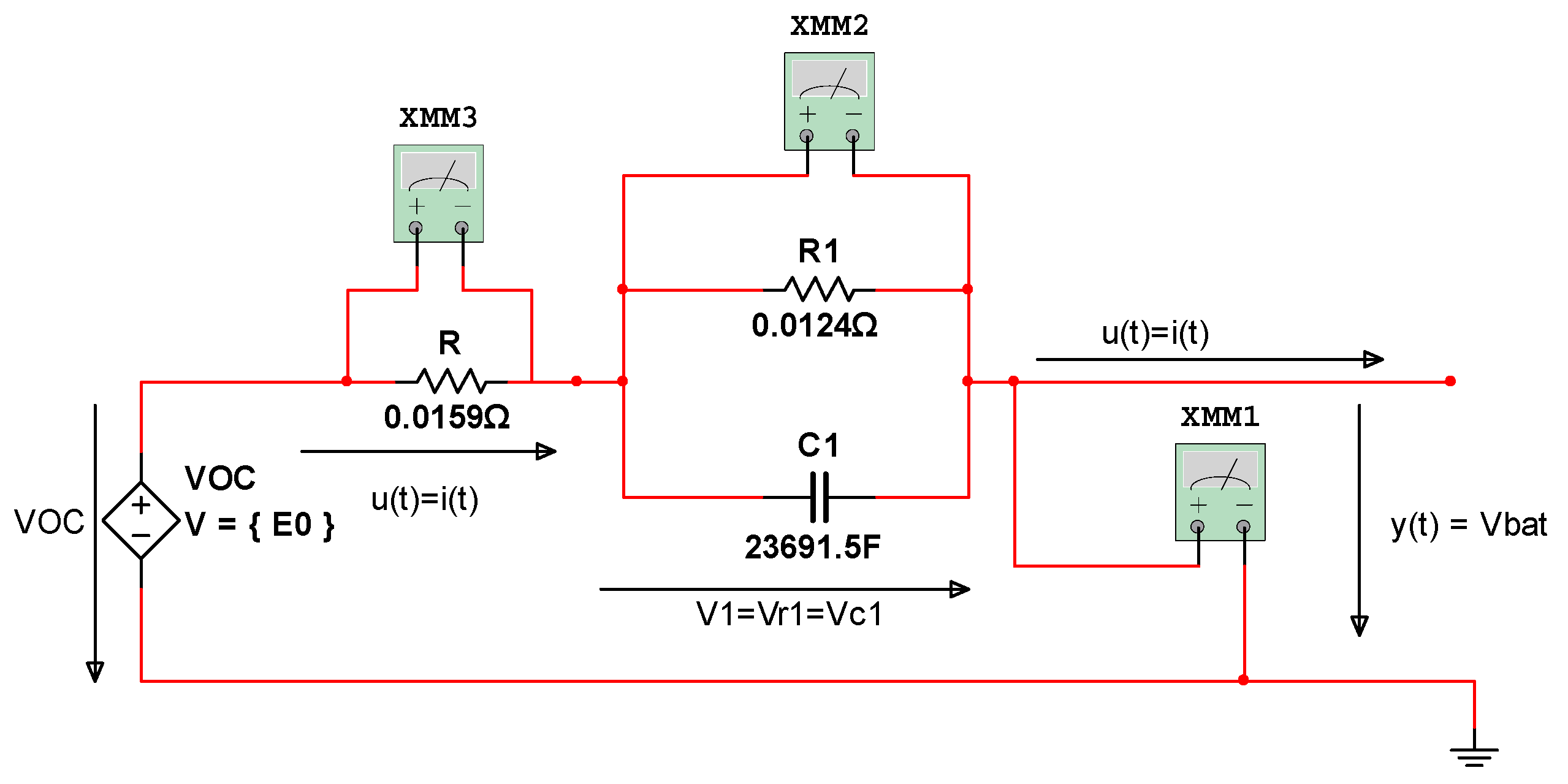
2.1. Li-Ion Battery—Equivalent Electric Circuit Schematics

For a better understanding of the battery model concept and further developments for the design and implementation of state estimation (SOC) algorithms, a first-order RC equivalent circuit model (ECM) was chosen [12]. This straightforward model has been proven to be efficient and well suited in real-time implementations for many HEV applications. In the case study, for “proof of concept” and simulation purpose proposes a Li-ion cobalt oxide ECM battery model with a nominal capacity of 6.6 Ah and a nominal cell voltage of 11.1 V for a possible integration into a battery pack of a hybrid electric car. The electronic schematic of the battery cell built in a NI MULTISIM 14 Editor is shown in Figure 1. The values of the components are also shown for each component, where R represents the internal resistance of the battery, assumed for simplicity purposes to have the same values for the charging cycle (the input current u(t) = i(t) < 0), Rch = 15.9 mΩ, and for the discharging cycle (u(t) > 0), Rdsch = 15.9 mΩ. Both components of the parallel bias cell, the resistor R1 and the capacitor C1, play an essential role in ensuring the fast dynamics of the adopted model. For the simplicity of the model, it is assumed that they have constant values, so they do not depend on temperature. The OCV represents the open circuit voltage of the battery (Thevenin voltage of the ECM model), highly nonlinearly dependent of SOC (state variable x1); V1 (state variable x2) denotes the polarization voltage of the R1C1 cell, and the output voltage y(t) = Vbat represents the terminal output voltage of the Li-ion battery.

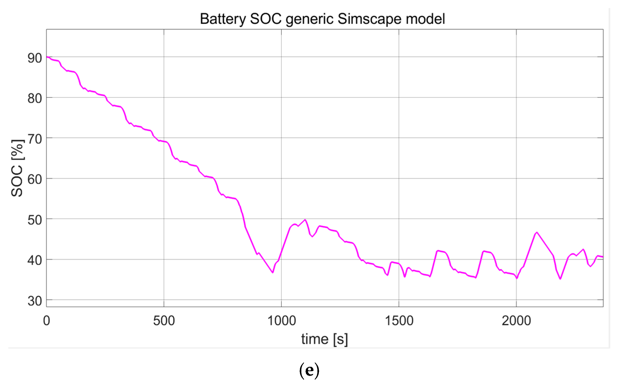
2.2. Li-Ion Battery—Simulink Simscape Rint Model Simulation

A Simulink Li-ion cobalt oxide generic battery model is proposed as a valuable tool for model validation as long as it is widely used for Simulink simulations in the automotive industry as a viable alternative to the old NREL ADVISOR simulator [31,32]. For “proof of concept” and simulation purposes, we selected a pre-set Li-ion cobalt oxide (LiCO2) Rint Simscape generic model of 6.6 Ah and 11.1 V rated nominal voltage, with the setup shown in Figure 2a–d. Each of these figures comes with one of the following pieces of information, namely, the Simscape model of the battery experimental setup shown in Figure 2a, a Li-ion battery setup with the initial conditions for SOC (90%) and ambient temperature (20 °C), the characteristic curves for three constant discharging current rates shown in Figure 2b. A two-cycle repeated New European Driving Cycle (NEDC) as an urban/suburban driving European regulated procedure test is shown in Figure 2c, which is valuable to proving the battery model SOC estimation accuracy and robustness performance. The Simulink simulation results (focused on the NEDC driving cycle current profile test and on the LIB SOC) are shown in Figure 2d,e. To analyze the robustness performance of the SOC estimators EKF and NOE in real-life driving operating conditions, three driving cycles current profile tests were used in the case study. The first procedure test consists of running an FTP-75 cycle followed by a highway fuel economy test (HWFET) cycle. The EPA FTP-75 is the standard federal exhaust emissions driving cycle in a city that uses an Urban Dynamometer Driving Schedule (UDDS) and consists of a series of tests defined by the U.S. Environmental Protection Agency to measure tailpipe emissions and the fuel economy of passenger cars (excluding light trucks and heavy-duty vehicles). The total test time for the FTP-75 is 2457 s (i.e., 40.95 min), the top speed is 56.7 mph, and the average speed is 21.4 mph. The distance is approximately 11 miles. The second current profile test NEDC is a European standard regulated procedure that combines the European Union Urban Driving Cycle and Extra-Urban Driving Cycle (EUDC), almost two times shorter than the FTP-75 test (i.e., approx. 20 min). Until now, it has been used on a large scale for emission certification of light duty vehicles in Europe and for HEV/EV energy consumption and regenerative breaking performance testing applications. Introduced in 2017, the second one-procedure test is a new European Worldwide Harmonized Light Vehicle Test Procedure (WLTP) including the version WLTC, which comes up with substantial methodology improvements to NEDC. It has the ability to test vehicles under conditions that are more realistic and better mimic on-road performance. For the case study, NEDC is suitable enough for the choice of a HEV Small Car (SMCAR) of 75 Kw rated power applications. The MATLAB simulation results shown in Figure 2c–e for the NEDC procedure test are completed in Section 2.6.3 with the performance of SOC estimation and battery terminal voltage prediction. This performance is obtained by using a high SOC accuracy Extended Kalman Filter (EKF) LIB SOC estimator and reveals the EKF SOC estimator effectiveness, demonstrating its popularity gained over the years as the most suitable SOC estimator for real-time deployments of many HEV applications, for whose parameter fine-tuning values and design are presented in Appendix A [11,14,15].

2.3. Li-Ion ECM RC Continuous Model in State-Space Description

The proposed first-order ECM RC Li-ion battery model can be easily implemented in a state-space representation by two first-order differential equations, one for the battery state-of-charge, designated as state variable x1, to describe the remaining battery capacity Q r e m after discharging the battery, and second one that describes the fast dynamics of the RC polarization cell, designated as state variable x2. The state space of the equivalent model is combined with a third static output–states–input equation to produce the battery terminal voltage y = Vbat, well known as a single-input and single-output (SISO) model. The last equation of the battery model is also a combination of a highly nonlinear function representing the open-circuit voltage (OCV), known also as Thevenin voltage, and the voltage dropped on the RC polarization cell. Finally, this combination generates the terminal battery voltage designated by output variable y.
The whole Li-ion battery model (LIBM) provided by Equation (1) excels in its simplicity, high capability of capturing the entire dynamics of the battery, ease in real-time implementation, and usefulness as a form of support to build the proposed state estimation algorithms:
d x 1 d t = η Q n o m u t ,   u t 0 ,   f o r   b a t t e r y   d i s c h a r g i n g , u t 0 ,   f o r   b a t t e r y   c h a r g i n g
d x 2 d t = 1 R 1 C 1 x 2 + 1 C 1 = 1 T 1 x 2 + 1 C 1 ,   T 1 = R 1 C 1 s ,   d e n o t i n g   t h e   t i m e   c o n s t a n t
y = h x 1 x 2 R u t ,   h x 1 = O C V S O C = k 0 k 1 1 x 1 k 2 x 1 + k 3 ln x 1 + k 4 ln 1 x 1
where k 0 , k 1 , k 2 , k 3 , k 4 represent the coefficients of the combined model that is well known as the Shepherd, Unnewehr universal, and Nernst combined model [13,14,15]. Their values are estimated by using the least squares errors for a curve fitting identification method that is based on the data extracted from the manufacture OCV specifications sheet of the Li-ion battery selected for this case study [9,10,11,12,13]. In the LIBM described by the set of Equations (1)–(3), the input variable u t = i t has the physical denotation of a DC instantaneous current that flows through the battery, and the physical meaning for output variable y t = V b a t t is a DC instantaneous terminal battery voltage. Moreover, T 1 = R 1 C 1 s represents the time constant of the polarization R 1 C 1 cell to describe the fast battery dynamics. To simulate and validate the LIBM and to demonstrate the effectiveness of the real-time SOC estimators that are developed and implemented in an attractive MATLAB Simulink software environment, as is shown in the following sections, the nominal values for the LIBM ECM parameters, namely, for R, R1, C1, and the coefficients of nonlinear function OCV(SOC), are similar to those used in [13,14,15]. The impact of the output terms of the nonlinear representation of OCV(SOC) function shown in Equation (3) in the combined model is significant in increasing the accuracy of the Li-ion battery EMC combined model, which proves also that it is amongst the most accurate formulations seen in the literature in the Evs/HEVs field.

2.4. LIBM ECM RC Discrete Time State-Space Representation

In most cases, to implement the battery model and SOC estimation algorithms, a compact discrete-time equivalent equation in matrix form is required, derived from the continuous-time description (1), (2), and (3) by using the first-order term Taylor series development, as follows,
x k + 1 = A x k + B u k ,   d x 1 d t x 1 k + 1 x 1 k T s ,   d x 2 d t x 2 k + 1 x 2 k T s
y k = C x k + D u k + g x 1
x k = x 1 k x 2 k = S O C k V 1 k ,   A = 1 0 0 1 T s T 1 ,   B = η T s Q n o m T s C 1 ,   C = k 2 1 ,   D = R
g x 1 k = k 0 k 1 1 x 1 k + k 3 l n x 1 k + k 4 l n 1 x 1 k
where Ts is the sampling time in [s], t = k T s , k Z + , x k = x k T s , y k = y k T s ,   u k = i k = u k T s = i k T s . Moreover, the constants η and Q n o m represent the coulombic efficiency for charging and discharging cycles, which for simulations are assumed to have same value for both cycles and nominal value of the battery capacity, respectively.
In the next sections, the nonlinear function g x 1 k is maybe linearized around an operating point to develop real-time SOC estimators, similar to in [13,14,15]. To analyze the behavior of the proposed LIBM EMC RC combined model for different driving conditions, such as urban, suburban, and highway, the FTP-75 driving cycle current profile tests were introduced in the previous Section 2.2.

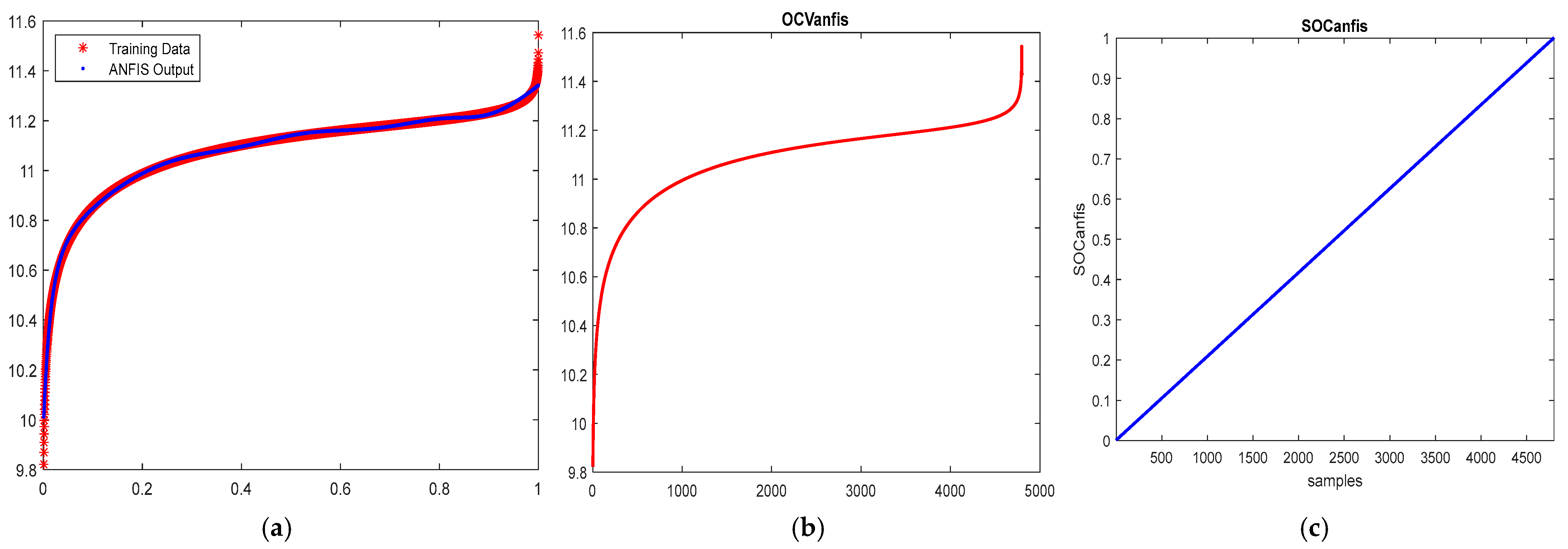
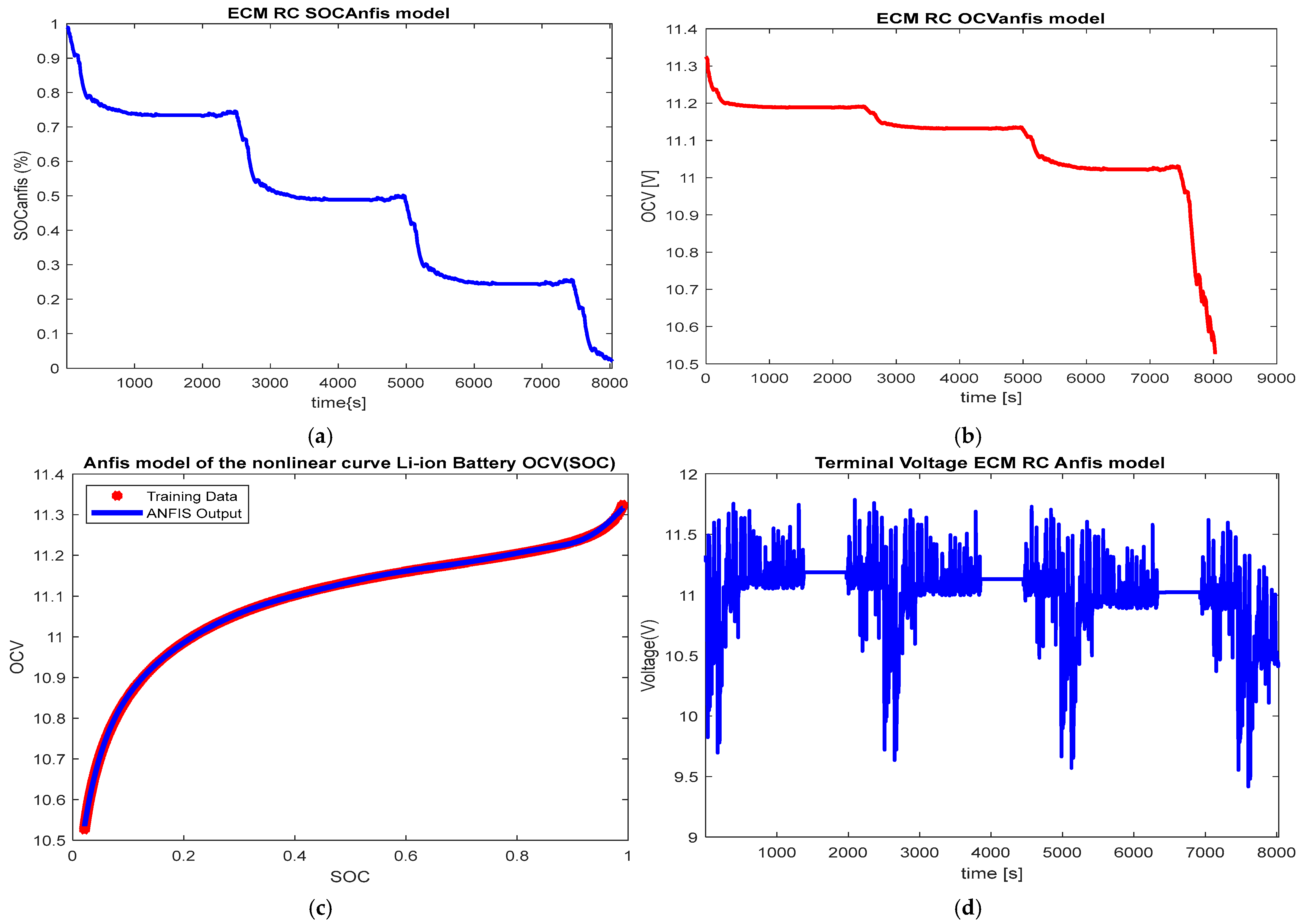
2.5. LIBM ECM RC OCV(SOC) ANFIS Model

Starting from the trainingData set, consisting of the collection of LIB SOC and OCV of input–output measurements generated from the LIB ECM RC model, a helpful specific MATLAB function anfis (trainingData) is required to build the LIB OCV output Sugeno fuzzy inference system (SFIS) and to tune the FIS parameters. Using a grid partition method, an FIS object is automatically generated, as is shown in Appendix A.2 [11,18]. The LIB trainingData set (SOC, OCV) is trained to generate the most accurate ANFIS model of the LIB ECM RC by using the fastest training algorithm, for example, a Levenberg–Marquardt “trainlm”, or others, on the basis of a combination of the least-squares error (LSE) and a backpropagation gradient descent method to model the training data. An important step in the training dataset is to choose the options, as a second argument of the MATLAB function syntax anfis (trainingData, options), and to tune a FIS using the specified trainingData and options, as one can see in the ANFIS algorithm summary steps from Appendix A.2. Beneficial for the implementer in using this MATLAB function is its excellent flexibility in the selection of an initial FIS object for tuning, validation, and overfitting prevention in training data; its training algorithm options; and its ability to display training progress information. Currently, remarkable research in the artificial intelligence (AI) field is conducted to develop a strong theoretical background related to stochastic, machine learning, and deep learning models using shallow or deep neural network architectures, fuzzy logic design, and the ANFIS modelling approach, helpful in developing new and suitable algorithms and techniques for real-time implementation in the most attractive and comprehensible software programming platforms, such as MATLAB, Simulink, and Phyton, in an extensive palette of HEV/EV applications [11,19]. In Appendix A.2 is a summary of the most significant MATLAB code key lines, beneficial for MATLAB readers and implementers for fast implementation and online generation of the ANFIS models entirely on the basis of the input–output measurement dataset suggested in [11,19]. The MATLAB simulation results are depicted in Figure 3a–c, for the OCV(SOC) ANFIS model during the training phase (a), for the LIB ECM RC OCV(SOC) model (b), and for LIB SOC for a complete discharging cycle of the battery (c). Figure 3a reveals a very accurate OCV(SOC) ANFIS model of LIB, a model that is required to build all four accurate SOC estimation algorithms in the following sections.
In the next developments presented in the following sections and subsections, the ANFIS OCV(SOC) battery model should cover the entire operating range for battery SOC, approximately between 0.001 and 0.999. In all developments in the case study, the Li-ion battery was tested for all three input current profiles mentioned in the previous section, namely, FTP-75, WLTC, and NEDC driving cycles. Thus, using an FTP-75 driving cycle, a full battery discharge occurs for a total duration of 8030 s, to be exact, equivalent to repeating 3.2 times the standard FTP-75 discharge current profile (2478 s), as shown in Figure 4a–d. The SOC for a full discharge battery is revealed in Figure 4a. Figure 4b presents the evolution of the battery OCV over the same period of time as for SOC in Figure 3a. The MATLAB simulations result during training phase to build the most accurate ANFIS battery model OCV(SOC), which is depicted in Figure 4c. A careful analysis of this result reveals that the OCV(SOC) nonlinearity described in Equation (3) was approximated with high accuracy by a smooth ANFIS model. The following developments mainly focus on the OCV(SOC) ANFIS model. Figure 4d shows the evolution of the battery terminal voltage on the same duration as is in Figure 4a–c.

2.6. EKF SOC Estimator for the LIBM ECM RC Model in Discrete Time State-Space Representation and Model Validation

The EKF SOC LIB estimator is the most popular state estimator, being a very strong state estimation tool used by implementers in various applications that cover almost all fields. The main steps of this algorithm are briefly presented in Appendix A.1 to provide a good insight for readers and implementers that is inspired from the fundamental research works in this field [13,14,15].

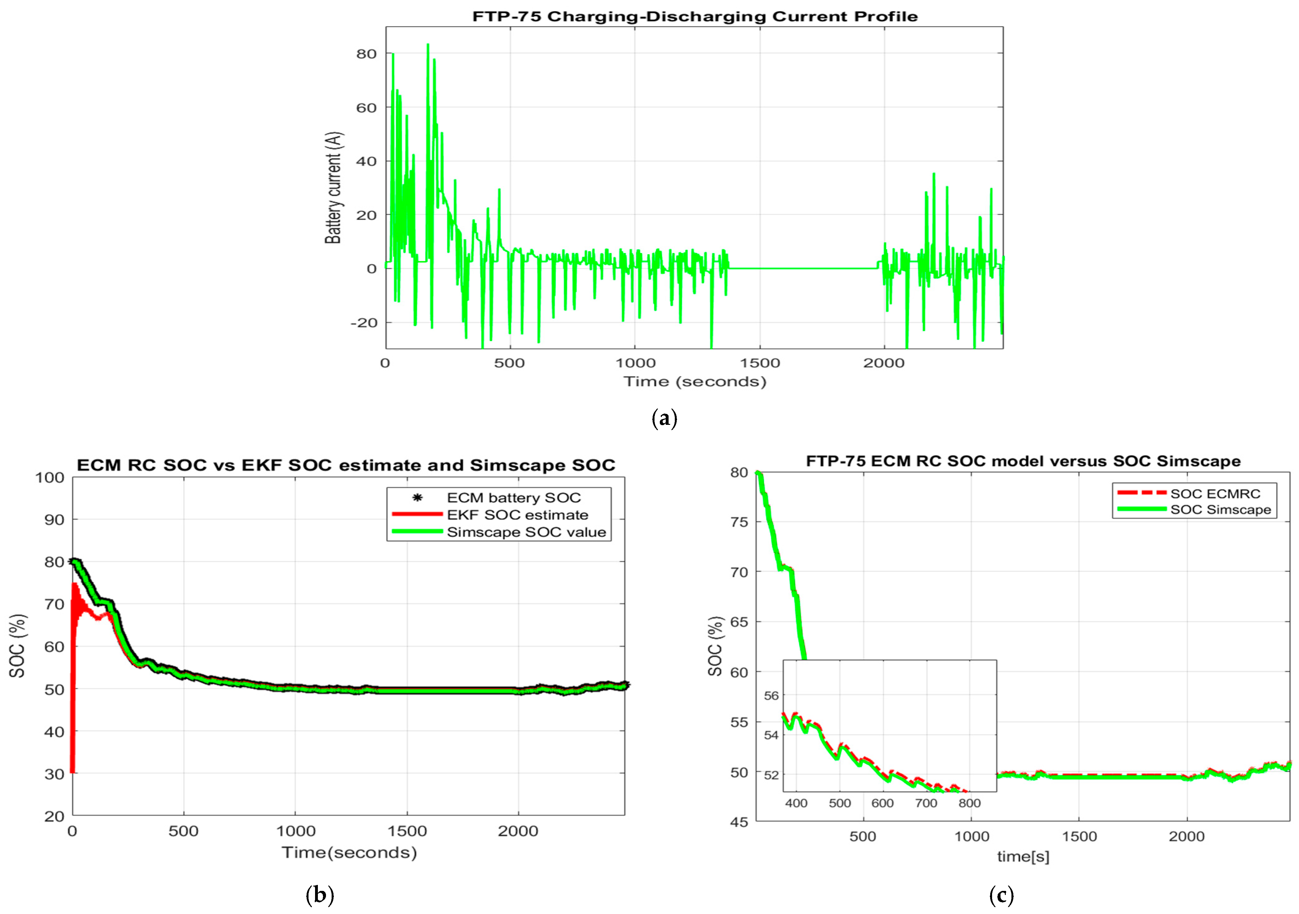
2.6.1. FTP-75 Driving Current Test Profile

The FTP-75 driving cycle for the input current profile is shown in Figure 5a. Figure 5b presents the MATLAB Simulink simulation result of the EKF SOC estimate versus the SOC Simulink generic model value and the actual SOC value for the LIB ECM RC model. Additionally, since Figure 5b shows on the same graph the actual SOC value of the LIB ECM RC model, EKF SOC estimated value, and Simscape SOC value, it is helpful for performance comparison and model validation. The curves in Figure 5c depict the LIB ECM RC SOC value and Simscape SOC extracted value from the experimental setup presented in Figure 2a and provide valuable information that both values of the SOC were close enough to prove the validity of the proposed LIB ECM RC model. Figure 5d,e represents the residuals corresponding to the graphs shown in Figure 5b,c, respectively. From both residuals, we can extract information of genuine interest for validation of the ECM RC battery model, such as that shown in Figure 5d, where the percentage of the SOC error between the estimated EKF value and the actual LIB ECM RC model value was under 0.22% compared to 2%,which is a typical value reported in the literature of the field; thus, these results validate, without a doubt, the accuracy and the robustness of the initial “guess value” of LIB ECM RC SOC value of the proposed EKF SOC estimator built on the accurate Li-ion battery model, having as a baseline the Simscape SOC generic model experimental setup values shown in Figure 5e. The percentage of the SOC error for the second residual from Figure 5e in the steady state (approximately after 500 s) tended towards zero and revealed a high accuracy SOC that validated the proposed LIB ECM RC model. The MATLAB simulation results from the last three in Figure 5f–h disclose the battery voltage (Figure 5f) and its highly nonlinear curve fitting OCV to battery SOC (Figure 5g). For a better insight of the charging and discharging cycles of the battery, we see that the SOC in Figure 5h corresponded to a complete discharging cycle (4000 s) at approximately a 1C discharging rate for a constant current u(t) = 6 A.

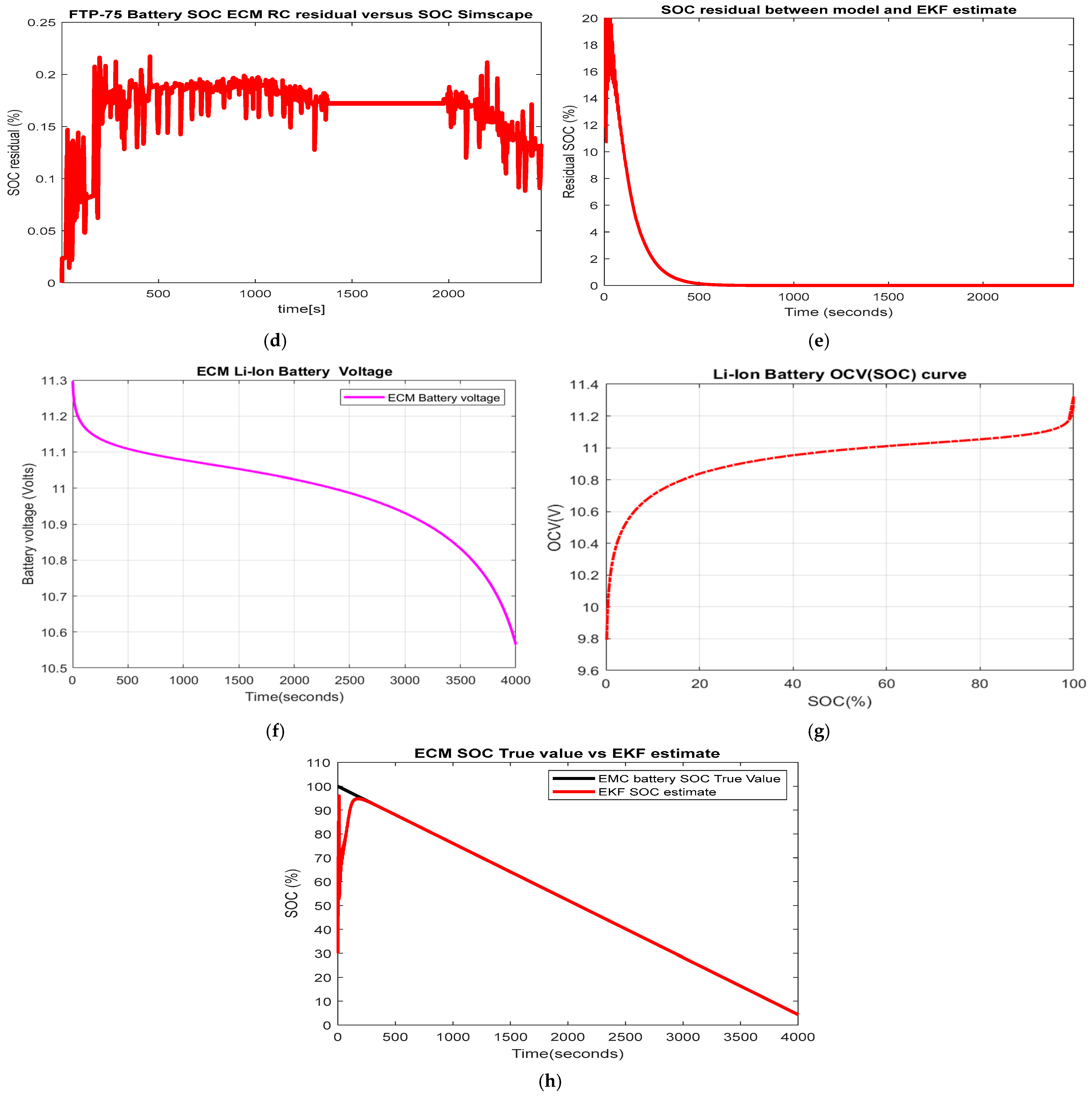
2.6.2. WLTC Class 3 Driving Current Test Profile

The WLTC class 3 driving cycle profile is a chassis dynamometer test used to determinate the emissions and fuel consumption from light-duty vehicles. It is used for all HEVs and EVs with a power mass rate (PMR) greater than 34 and the maximum speed exceeding 120 km/h for class 3a or smaller than this limit for class 3b [33,34,35]. Moreover, all the WLTC cycles are part of the Worldwide Harmonized Light Vehicle Test Procedures (WLTP) introduced in Europe since 2017 [33]. The WLTP was conceived to replace the European NEDC-based procedure “for type approval testing of light-duty vehicles with the transition from NEDC to WLTP occurring over the period 2017–2019” [33]. In comparison to the NEDC European standard procedure test, the WLTC procedure test is more realistic when simulating usual real-world driving conditions and also is more dynamic, covering a large spectrum of engine working states. Additionally, the WLTC class 3 obtained a high level interest for its introduction into vehicle certification in Japan. For interested readers, some details on the driving cycle diagrams on output displacement ( km ), velocity ( km / h ), and acceleration ( m / s 2 ) in speed in km/h for all three classes (classes 1, 2, and 3) and details on these are found in [33,34,35]. The case study provided features of the proposed Li-ion battery model, such as simplicity, high accuracy, and ability for real-time implementations, which were validated, without a doubt, by the model behavior in terms of the impact of all three driving cycle procedures tests, the quality of the SOC estimation and terminal voltage prediction accuracy performance, and the robustness of the estimators built using such a model. The impact of the WLTC-class-3 current profile test on the overall performance of the EKF estimator was revealed by a rigorous analysis of the MATLAB simulation results shown in Figure 6. The WLTC class 3 is suggested in [34] on the basis of the data collected from an acceleration diagram in m s 2   , which were obtained from an input signal, such as a displacement in ( km ) or velocity in ( km / h ). To obtain an approximate current profile for the Li-ion battery required to charge or discharge the battery during a cycle or repeated cycles, the acceleration signal was amplified by a proportional correction factor. This correction factor can be defined on the basis of the power balance, i.e., the power required by the Li-ion battery to match the rated electric motor’s power. A rough driving cycle current profile test WLTC class 3 is shown in Figure 6a. The impact of this test can be seen in Figure 6b by comparison of the battery model SOC and battery Simulink generic model. In Figure 6c, we compare the EKF terminal predicted voltage and the true value of the terminal voltage of the model, and similarly, in Figure 6f, we show the EKF SOC estimate and the SOC true value of the battery model. The results of these comparisons were obtained by a simple visualization of the corresponding residuals from Figure 6d,e,g. All three residuals revealed an excellent accuracy performance and robustness of the EKF SOC estimator to the changes in an initial “guess value” of SOC from 80% to 40% with almost zero steady-state errors in Figure 6e,g, and smaller than 1.2% in Figure 6d. Therefore, even though this test was much more aggressive than the other two competitors, FTP-75 and NEDC, the results proved that the EKF SOC estimator had excellent performance (SOC estimation accuracy and terminal voltage prediction, as well as an excellent robustness to this aggressive driving cycle).

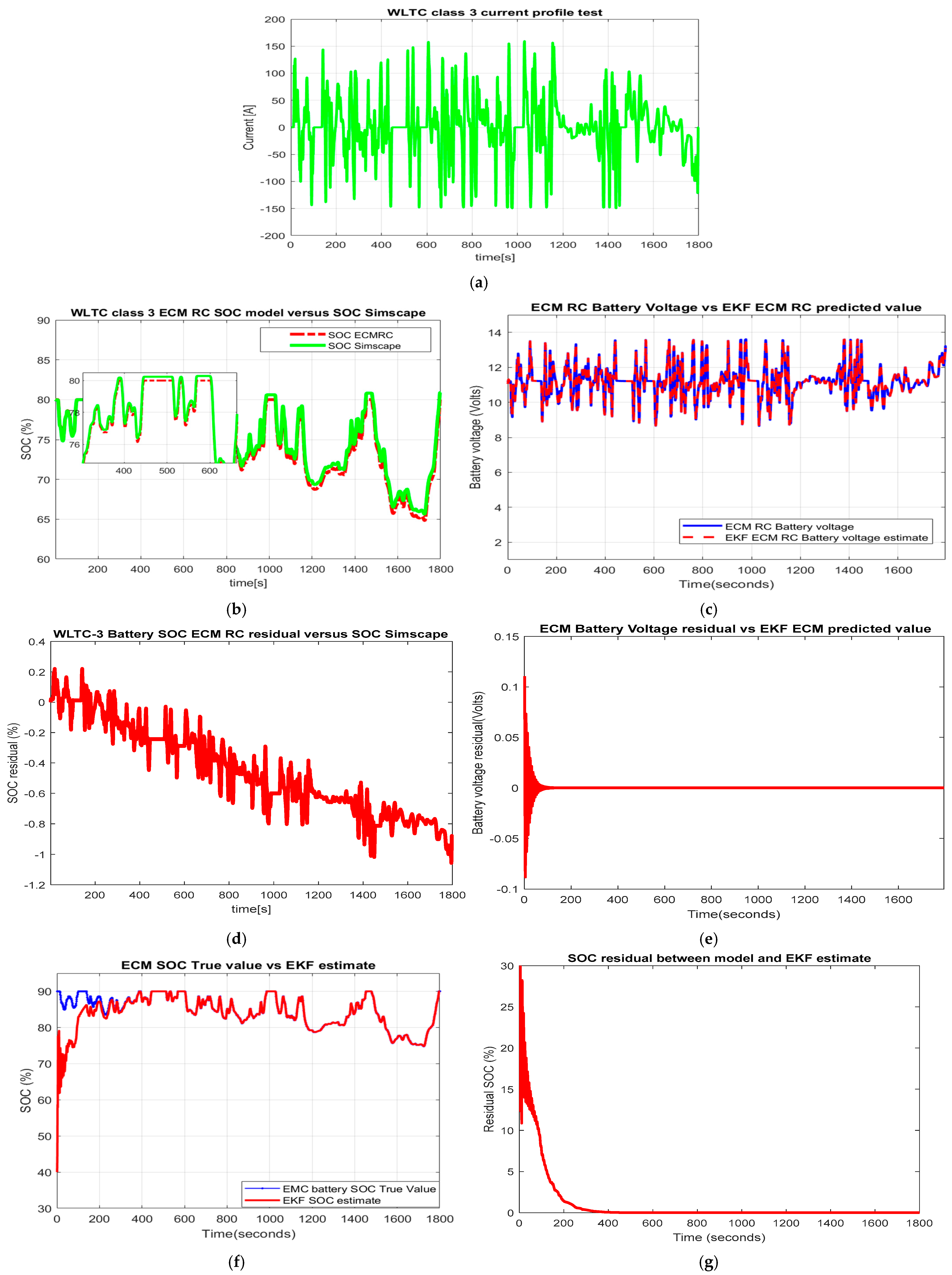
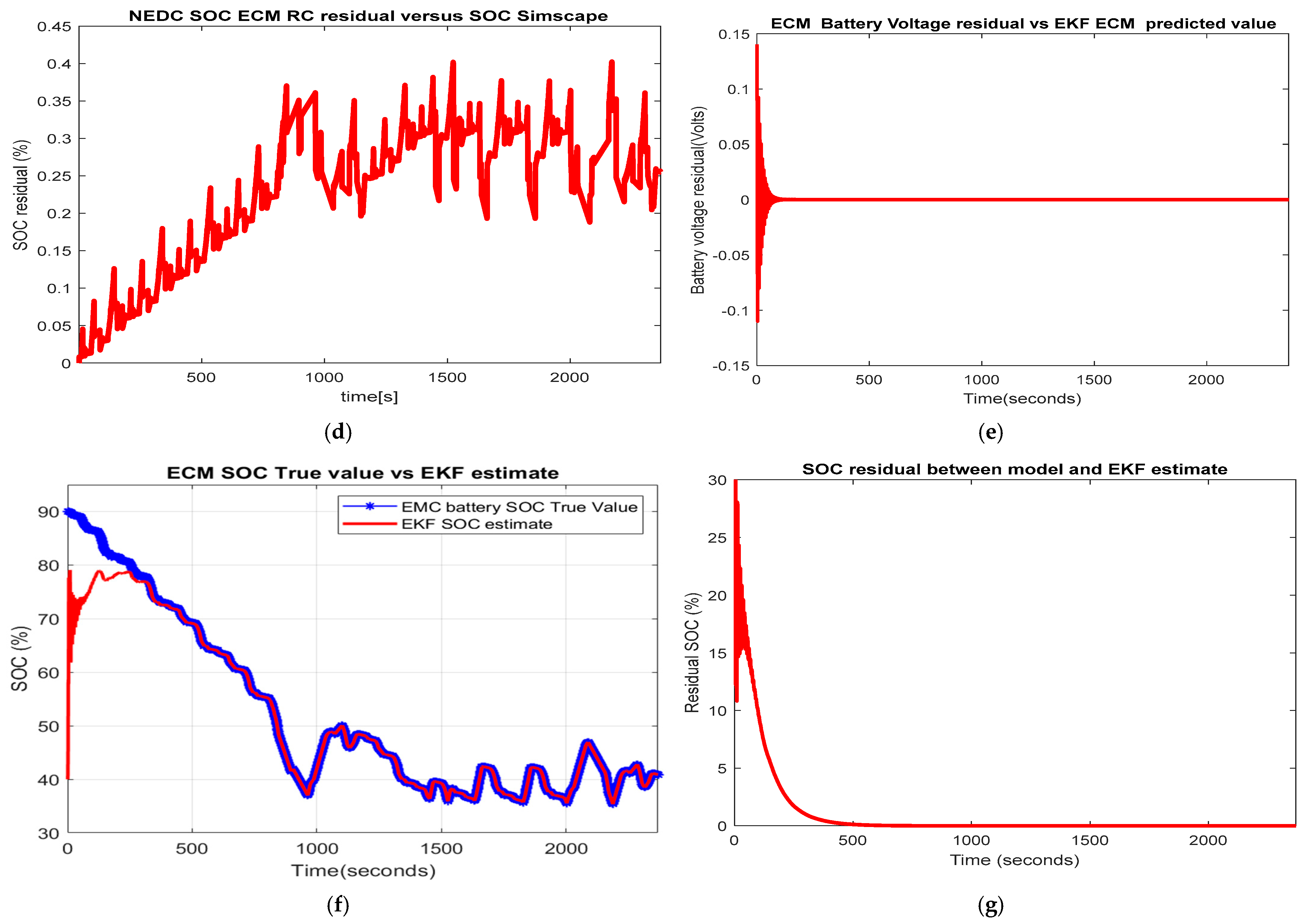
2.6.3. NEDC Driving Current Test Profile

Similarly, as for WLTC class 3 described in Section 2.6.2, in Figure 7a–g are depicted the MATLAB Simulink results for the European driving cycle current profile test NEDC. The NEDC driving cycle current profile test is provided in Figure 7a. Its impact on the overall performance of the EKF estimator in terms of the SOC accuracy and terminal voltage prediction is visible in Figure 7b,c,f by comparison with the battery model SOC and battery SOC of the Simulink generic model (Figure 7b) of the EKF terminal predicted voltage and the true value of the battery model terminal voltage (Figure 7c), and finally of the EKF SOC estimate and the battery model SOC true value shown in Figure 7f. A simple visualization of the corresponding residuals depicted in Figure 7d,e,g indicates a great performance of the EKF SOC estimator and terminal battery voltage predictor in terms of accuracy and robustness, very close to the WLTC class 3 driving cycle current profile test. Therefore, the impact of changing the FTP-75 driving cycle by the NDEC procedure test is strongly attenuated by the ability of the EKF SOC estimator and terminal voltage predictor to perform accurately, to be robust, and to perform very well in real-time implementations.

2.6.4. EKF SOC Estimator and Terminal Voltage Prediction Using OCV ANFIS Mod–l–MATLAB Simulink Simulation Results for FTP-75 Driving Cycle Current Profile Test

On the basis of the Li-ion battery OCV ANFIS model, for the same FTP-75 driving cycle current profile test developed in Section 2.6.1, the accuracy and the robustness of the EKF SOC estimator and terminal voltage prediction to changes in the SOC initial value from 90% to 40% were revealed by the MATLAB simulations results shown in Figure 8a–c. In Figure 8a, we show the EKF SOC estimate of the ECM RC ANFIS model versus its true SOC value, and in Figure 6b, we disclose a high accuracy and estimator robustness to predict the battery terminal voltage. The SOC residual for the ANFIS model indicated an SOC percentage error smaller than 0.7%, thus being a very good level of performance compared to those reported in the literature, typically at approximately 2%. Additionally, the EKF SOC estimator based on the American FTP-75 EPA standard procedure was very robust in terms of the changes of operating conditions. These changes were the result of replacing the FTP-75 driving cycle by NEDC or WLTC class 3, well known as the most representative regulated procedure tests used in Europe for gas emission certification of HEVs/EVs from the automotive industry.. Intentionally, the initial value for SOC for the battery model was changed from 80% to 90% to reach the target of 60% of normal operation. A rigorous analysis of the behavior of the EKF SOC estimator to all three driving cycle procedure tests revealed an excellent robustness of the EKF SOC estimator, and additionally, this was very accurate in the SOC estimation and terminal voltage prediction. Moreover, it was robust to changes in the initial “guess” value for LIB ECM SOC. Its capability for real-time implementation in a large number of HEV/EV applications recommends this traditional algorithm as a strong SOC estimator.

2.7. NOE SOC Estimator for the LIBM ECM RC Model in Discrete Time State-Space Representation

A viable alternative to the traditional SOC EKF estimator is proposed for comparison purposes for one of the most robust nonlinear estimators, namely, an LIB SOC adaptive nonlinear observer estimator (ANOE) [5]. The main steps of this algorithm are suggested by [5] and are summarized in Appendix B, being valuable for readers and implementers for a better understanding and implementation. The MATLAB simulation results are displayed in Figure 9a–d for the original LIB ECM RC model described by Equations (4)–(7), and as shown in Figure 10a–e, similar results were obtained by replacing in the LIB ECM RC model the nonlinear function OCV(SOC) by an ANFIS model developed in a previous section.
For performance comparison purposes, in Table 1, we present the MATLAB simulation results collected from both traditional algorithms in terms of convenient statistics, such as root mean square error (RMSE), mean square error (MSE), and the mean absolute error (MAE), all calculated by using the specific MATLAB functions, such as RMSE (estimates, observations, “all”), MSE (estimates, observations, “all”), and MAE (estimates, observations, “all”). One of these statistics, MSE, is used to measure the training performance of the data set for both intelligent estimators, developed in Section 3, and thus is beneficial for performance comparisons of all four estimators and then to choose the most appropriate and accurate estimator for these kinds of applications.

3. Shallow SISO and MISO Neural Network Estimators for SOC and Terminal Voltage of Li-Ion Battery

Compared to deep learning neural networks (DLNNs) that have multiple hidden layers in their architecture, their number being a key parameter to adjust the increase in accuracy of the target estimation, shallow neural networks (SNNs) have only one hidden layer with a reasonable capacity to approximate any non-linear function but with some limitations to improve prediction accuracy for all types of applications [26]. A single-input single-output (SISO) SNN estimator is a feedforward neural network with a simple architecture consisting of an input layer with a single-input predictor (feature), a single hidden layer with multiple neurons, and an output layer with a single-output target (response [22,23,24,25,26]). A multiple-input and single-output (MISO) SNN includes into its architecture an input layer with multiple predictors, a single hidden layer with a different number of neurons, and an output layer with a single-output target [25]. In the case study, we chose two SNN architecture configurations. The first was a SISO nonlinear autoregressive SNN with exogenous inputs (NARX) that estimates Li-ion battery SOC on the basis of the input–output measurement data set, namely, battery discharge current u(t) as an input predictor, namely, an FTP-75 standard current profile, and the estimated SOC of the battery as the output target y(t) [22,24]. The second is a MISO SNN used to predict the LIB terminal voltage on the basis of the input–output measurement data set, consisting of two input predictors, namely, LIB SOC (u1(t)) and battery discharge current (u2(t)) and an output target represented by the battery terminal voltage (y(t)) [26]. This section reveals the estimation accuracy of both outstanding SNN architectures that excel in low complexity and simplicity of real-time implementation in an attractive and friendly MATLAB programming environment for a specific application in HEV/EVs presented in the case study.

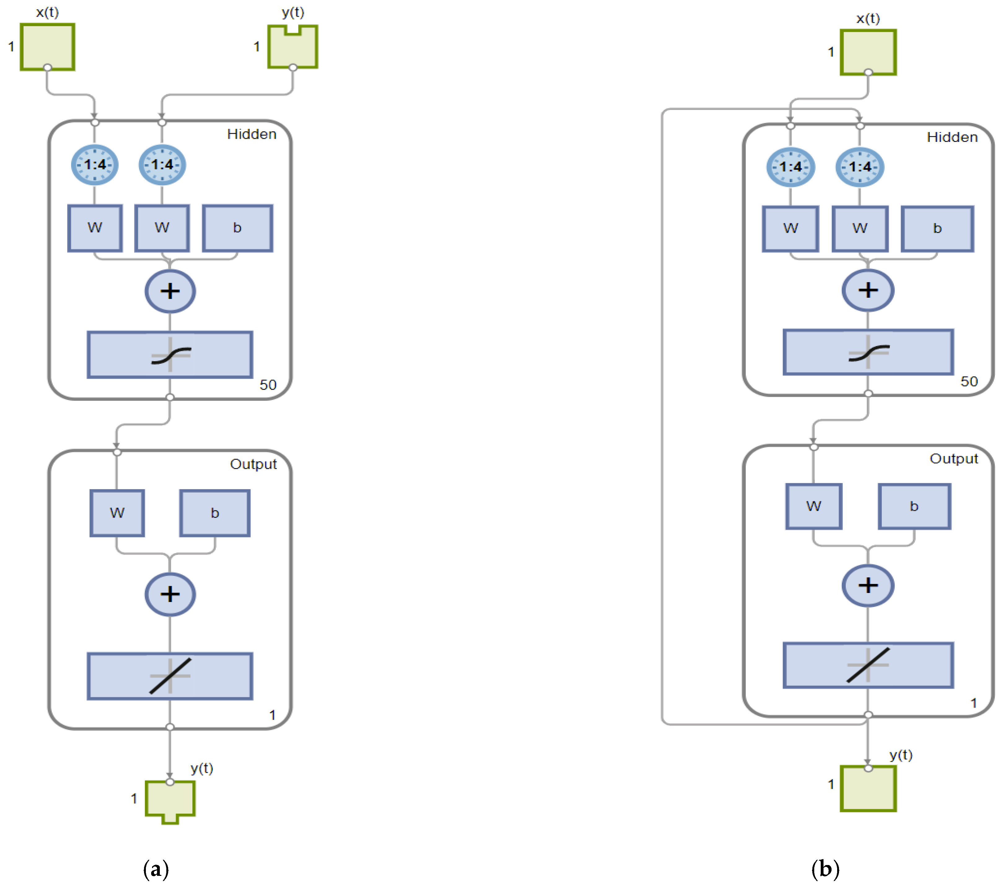
3.1. Time Series NARX Feedback SNN as LIB SOC Estimator—MATLAB Design and Implementation

The NARX architecture is usually encountered in multiple modelling time series and is nothing more than a simple recurrent dynamic network with feedback connections spanning various network layers [22,24]. The NARX model is based on the following linear ARX model [23]:
y t = f y t 1 , y t 2 , , y t n , u t 1 , u t 2 , , u t m
where the value of the output target signal y t depends on previous values of the output signal y t 1 , y t 2 , , y t n and on previous values of an independent (exogenous) input predictor signal u t , i.e., u t 1 , u t 2 , , u t m , where m and n are the number of the input and output measurement data set samples, respectively. The NARX model given by Equation (8) can be implemented in a MATLAB Simulink R2022b software environment as a dynamic recurrent feedforward neural network applied to approximate the function f, with various details shown in [22,23,24,25,26]. Applications of the NARX SSN architecture include its use as a predictor to predict the next value of the input signal, nonlinear filtering, where the target output is “a noise-free version of the input signal” and modeling nonlinear dynamical systems [22,24]. Two main configurations for the NARX architectures are reported for training in the literature, well explained in [22,23,24]. In general, the output variable value for NARX SNN configurations can be considered as an estimate of the output variables of certain nonlinear dynamical system models. First, configuration is a parallel configuration for which the output value is fed back to the input of the feedforward neural network integrated in the standard NARX architecture. As long as the true output value of the NARX SNN configuration is available during the network training phase of the network, a revolutionary series parallel architecture, which uses the true output instead of feeding back the estimated output, proves itself as having two significant advantages, namely, a high accuracy of the input to the feedforward network and a purely feedforward architecture such that a static backpropagation can be used for training [22,24]. The main objective of this subsection is to build the NARX estimator for LIB SOC estimation, starting by using a series-parallel architecture in open loop and then closing this architecture to exploit the features of a parallel architecture, such as is presented in Figure 11 and Figure 12a,b. The input–output data set was generated and collected from the LIB model, represented by Equations (4)–(7) at the sampling interval of 1 s. Typically for designing any SNN, it is required for one to follow the standard steps, such as the following:
Step 1. Collect the input–output measurement data set (i.e., load one or many files, generate directly from the model in a main program, etc.).
Step 2. Create a neural network.
Step 3. Configure the neural network.
Step 4. Initialization of the weights and biases.
Step 5. Training phase of the data set (predictors and targets).
Step 6. Validate the neural network performance.
Step 7. Deployment of the neural network model (hardware implementation).
There are two inputs to the series-parallel network in open-loop configuration, x(t) and y(t) sequences, each one delayed by 4 s, wherein the training phase begins with the fifth data point, as is depicted in Figure 12a. To estimate the battery SOC, a series parallel NARX SNN was created by using a particular MATLAB function “narxnet”. In the hidden layer were used 50 neurons, and the training MATLAB function” trainlm” was used that is based on the fastest Levenberg–Marquardt training algorithm. The collected measurement data set was prepared by using the MATLAB function” preparets” [22]. It is noteworthy that the y sequence is considered a feedback signal, which is an input that is also an output (target) [22]. Later, when the loop is closed, the appropriate output will be connected to the appropriate input. From here, the NARX SSN is ready to be trained, using the following MATLAB code line [22]:
NARX_SSN_net = train (NARX_SSN_net, p, t, Pi)
A complete visualization of training results, training progress, and performance tabs appear in Figure 11. A statistic criterion assessment of the NARX SSN estimation performance employed the mean square error (mse), which reached approximately 2.304087353387711 × 10⁻⁸, revealing a very good performance. The NARX SNN diagrams for open loop and closed loop are shown in the Figure 12a,b, obtained by using the MATLAB code line [22]:
view (NARX_SSN_net)
Remark 1.
All the MATLAB simulations for training phase were performed for a NARX SNN series-parallel architecture (open loop). Thus, the main goal of this subsection was to fully create a NARX SNN in open loop architecture. Then, when the training phase was finished, we also included the validation and testing steps, and the NARX SNN open loop architecture was converted to a closed loop form for a “multistep-ahead prediction” [25]. Moreover, the R-values in the Simulink GUI, depicted in Figure 12c,f, were computed on the basis of the open-loop training results.
Finally, the NARX SNN closed loop (parallel) configuration could be used to perform an iterated prediction on the length of the testing samples time steps. The MATLAB “preparet” function was used to prepare the data such that the new configuration of NARX SNN in closed loop was loaded with both initial inputs and both initial outputs as initial conditions. The network structure was used to determine the way in which to divide and shift the data appropriately, with the details provided in [16,19]. Figure 12c shows the excellent accuracy of the LIB SOC estimate (target, red curve) versus the LIB ECM RC model SOC (the output y = SOC, blue curve) during training phase, as a response to the FTP-75 driving condition current profile (the input predictor, x(t) = u(t)). Figure 12d shows the NARX SNN state performances (gradient, momentum, and validation fail). The best mse validation performance of the NARX SNN open-loop configuration was reached faster after epoch 151 and was revealed in Figure 12f, and the errors between the SOC estimated value and SOC true target value generated by the LIB EMC RC model given by Equation (4) are shown in Figure 12g (error autocorrelation) and Figure 12h (error histogram). A rigorous analysis of the NARX SNN performance by comparison with traditional estimators, namely, EKF SOC and NOE SOC, implemented in a previous section, revealed the excellent accuracy of the LIB SOC estimate, slightly superior to the last two SOC estimators. This outstanding result was confirmed by the residual steady state error from the bottom graph shown in Figure 12c, which was almost zero.

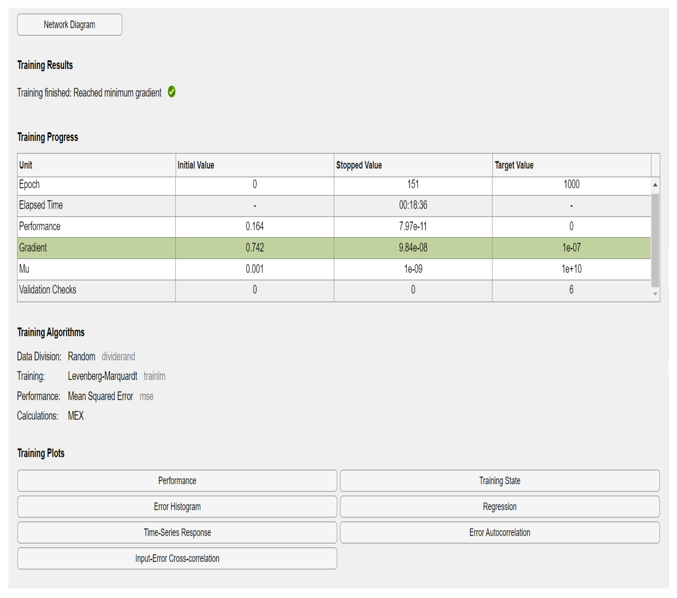
3.2. Shallow MISO Neural Network Terminal Voltage Estimator of LIB

Similar to NARX SNN, a reasonably simple shallow neural network (SNN) proved its ability to fit any practical function in any situation [25,26]. SNNs are widely used in control system modelling applications to match (fit, regression) or predict online and offline with high accuracy any output variable related through the control system model to certain input variables based on the input–output measurement data set. This kind of matching or prediction problem can be solved by using the MATLAB Simulink software package in two different ways [25,26]:
  • using the Simulink Neural Net Fitting app, which can be opened using the Simulink Toolbox “nftool” command, as a line in the MATLAB command window, or as a code line in script, as well as in a live script.
  • using command-line functions, as described in [25,26].
We preferred the second way due to its simplicity, user approachability, and flexibility in using command-line functions.
Inspired by [25,26], the following summarizes the most used command-line functions in a beneficial way and with better understanding given to the readers and implementers. Additionally, many more details can be found on the same MathWorks documentation site for MATLAB R2023a. The design steps and real-time implementation in MATLAB Simulink are almost the same as those defined for NARX SNNs in the previous subsection.
Step 1. Select the data for the case study generated by the Li-ion ECM RC battery model.
Step 2. Choose a training algorithm, preferably the fastest Levenberg–Marquardt backpropagation algorithm.
‘ ’ trainFcn = ‘trainlm’
Step 3. Create a shallow neural network (select the number of neurons in the hidden layer).
hiddenLayerSize = 25 (selected for the case study)
net = fitnet (hiddenLayerSize, trainFcn)
Step 4. Set up the dataset for training, validation, and testing phases (the implementer has the flexibility to select the percentages depending on the data set size).
net. divideParam.trainRatio = 0.7 (70%), (selected for the case study)
net. divideParam.valRatio = 0.15 (15%), (selected for the case study)
net. divideParam.testRatio = 0.15 (15%), (selected for the case study)
Step 5. Train the shallow neural network created at step 3.
[net, tr] = train (net, Predictor_X, Target_T)
Step 6. Test the shallow neural network trained at step 5, on the basis of the indexes set up at step 4.
Y = net (Predictor_X)
Error = gsubtract (Target_T, Y)
performance = perform (net, Target_T, Y), for the case study approximately 1.1081 × 10⁻⁴
Step 7. Visualize the shallow neural network tested at step 5, as is shown in Figure 13a.
view(net)
Step 8. Plots the graphs using the following MATLAB plot functions:
3.
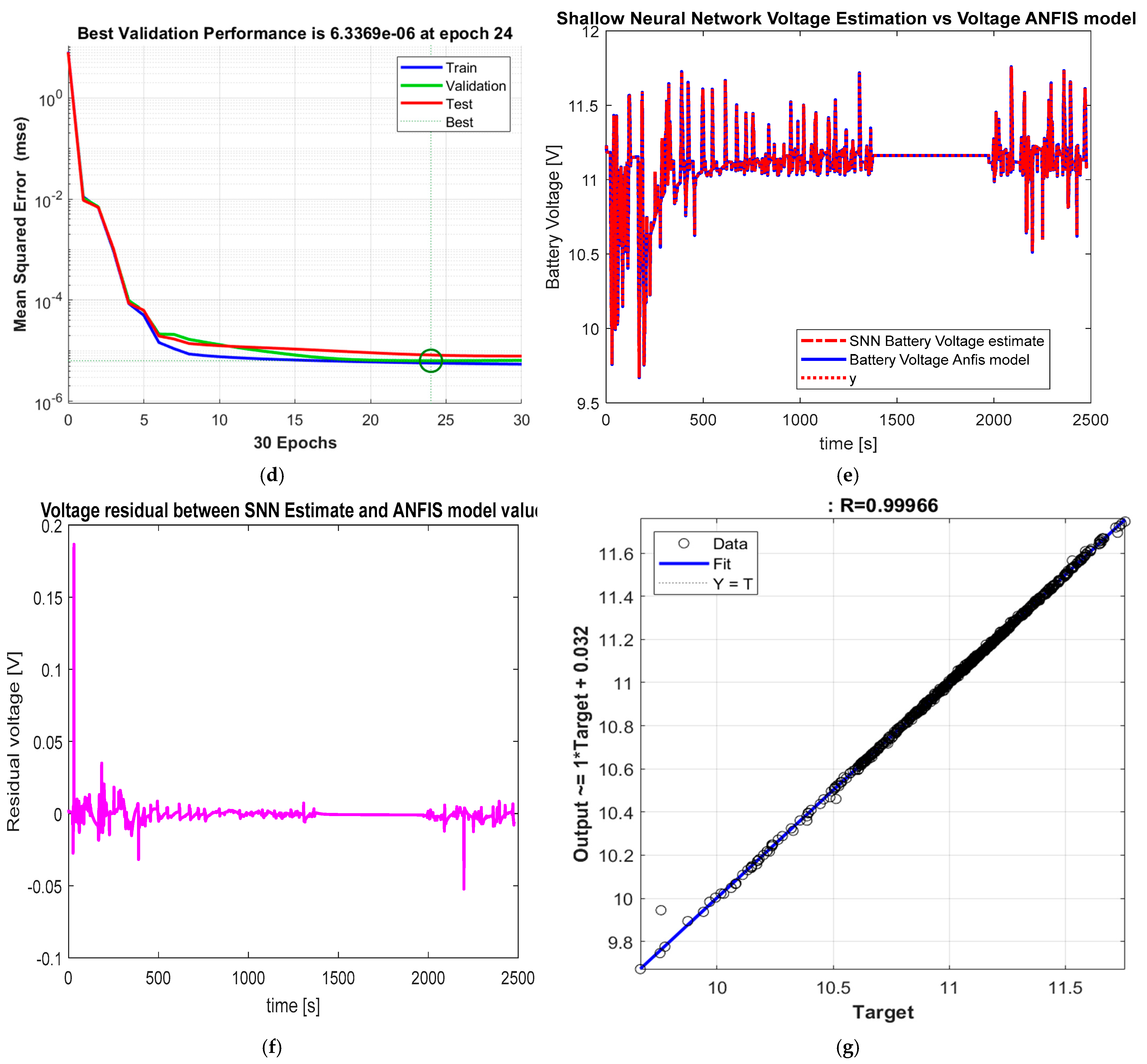
plotperform(tr) with the simulation results shown in Figure 13d;
4.
plottrainstate(tr), which is similar to the previous Figure 12d for NARX SNN;
5.
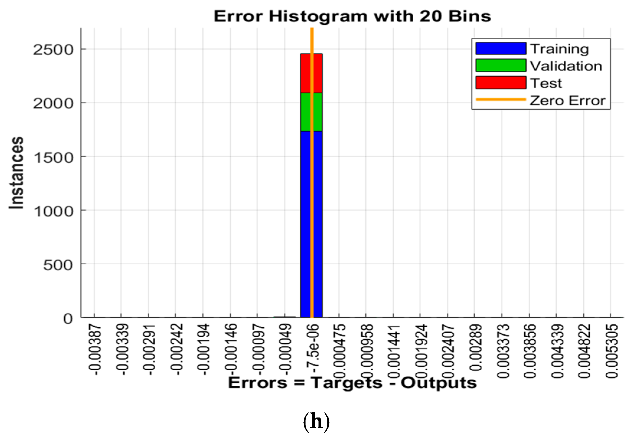
ploterrhist (Error) with the simulation result shown in Figure 13c;
6.
plot regression (Target_T, Y), as is depicted in Figure 13g;
7.
All these graphs have the same meaning as for NARX SNN in open-loop configuration, represented previously in Figure 12.
8.
Step 9. Analyze the results.
For the case study, the MATLAB simulation results presented in Figure 13e,f reveal the excellent estimation accuracy of LIB terminal voltage (Figure 13e); this valuable information was obtained from the residual voltage error depicted in Figure 13f, small enough (approximately less than 0.03 V) to be able to make a remark on the superiority of the SNN voltage terminal estimator compared to the traditional estimators (EKF and NOE) implemented in the previous section.
Step 10. Deployment of the SNN created, trained, validated, and tested for hardware implementation (FPGA board or simulator, microcontrollers, etc.).

4. Discussion

This research work provided us with a great opportunity to develop our skills to design, model, and develop SOC estimators of high accuracy, simplicity, robustness. The MATLAB simulations results revealed the great performance of SOC accuracy; the robustness to changes of “guess value” of a battery SOC from 90% to 30%; and the operating conditions in a harsh environment, assessed on the basis of the statistical criteria, such as RMSE, MSE, and MAE, or direct visualization of the graphs, especially of SOC residual errors such those from Figure 5d,e, Figure 9c and Figure 10c, that are less than 0.5% during the steady state, compared to 2% reported in the literature of the field. As shown in Table 1, three statistical criteria (RMSE, MSE, and MAE) are used for performance assessment. Their values provide valuable information on the most suitable SOC estimator or battery terminal voltage predictor, thus on an appropriate choice between EKF and ANOE estimators introduced in Section 2.5 and Section 2.7. It is worth mentioning the fact that for both intelligent LIB SOC and terminal voltage, the common statistical criterion for performance assessment is MSE. Therefore, it is necessary to find the most suitable SOC state estimator based on an accurate LIB model, such as the one proposed in the case study. The performance of each SOC estimator is validated through an extensive number of MATLAB simulations conducted on an experimental Simulink setup that generates for performance comparison purpose an alternative accurate Li-ion battery generic model. By MSE performance comparison, it seemed that the ANOE SOC estimator (MSE = 0.0031) performed in a slightly superior manner to the EKF SOC estimator (MSE = 0.0075) from a SOC accuracy perspective, with robustness to changes in the “SOC guess” value from 90% to 30%, smooth convergence, and a time response. Thus, by comparison with the NARX SNN SOC estimator (MSE = 7.97 × 10⁻¹¹) to the winner of the competition between ANOE SOC and EKF SOC, i.e., ANOE SOC (MSE = 0.0031), it was obviously the case that the NARX SNN SOC estimator outperformed the ANOE SOC estimator, and thus the most suitable SOC estimator for this kind of applications is the NARX SNN SOC deep learning estimator. However, from the battery terminal voltage prediction perspective, the winner of the competition is the EKF estimator, as long as MSE_ANOE = 1.885 × 10⁻⁴ vs. MSE_EKF = 5.07 × 10⁻⁵,thus a slight superiority. Finally, by comparing the same perspective of terminal voltage prediction, the MSE_SNN = 5.43 × 10⁻⁶ vs. MSE_EKF = 5.07 × 10⁻⁵ led the intelligent SNN terminal voltage estimator to become the winner of the competition. Overall, the most suitable SOC estimator and the best LIB terminal voltage prediction was the intelligent NARX SNN SOC deep learning estimator. Additionally, the intelligent NARX SNN SOC deep learning was dataset input–output measurement based, and thus it is implementable online and is suited for real-time HEV applications.

5. Conclusions

The main contributions involved in this research paper are highlighted in the following list:
(a)
Model selection—a pre-set Li-ion cobalt oxide (LiCO2) Rint Simscape generic model of 6 Ah and 11 V nominal voltage, ECM RC nonlinear model, simple, practical, accurate, easy to implement in real time in MATLAB environment, and validated using an experimental Simulink setup (Section 2.2).
(b)
Model hybridization including the most accurate ANFIS model of OCV(SOC) (Section 2.5, Appendix A.2, Figure 3 and Figure 4).
(c)
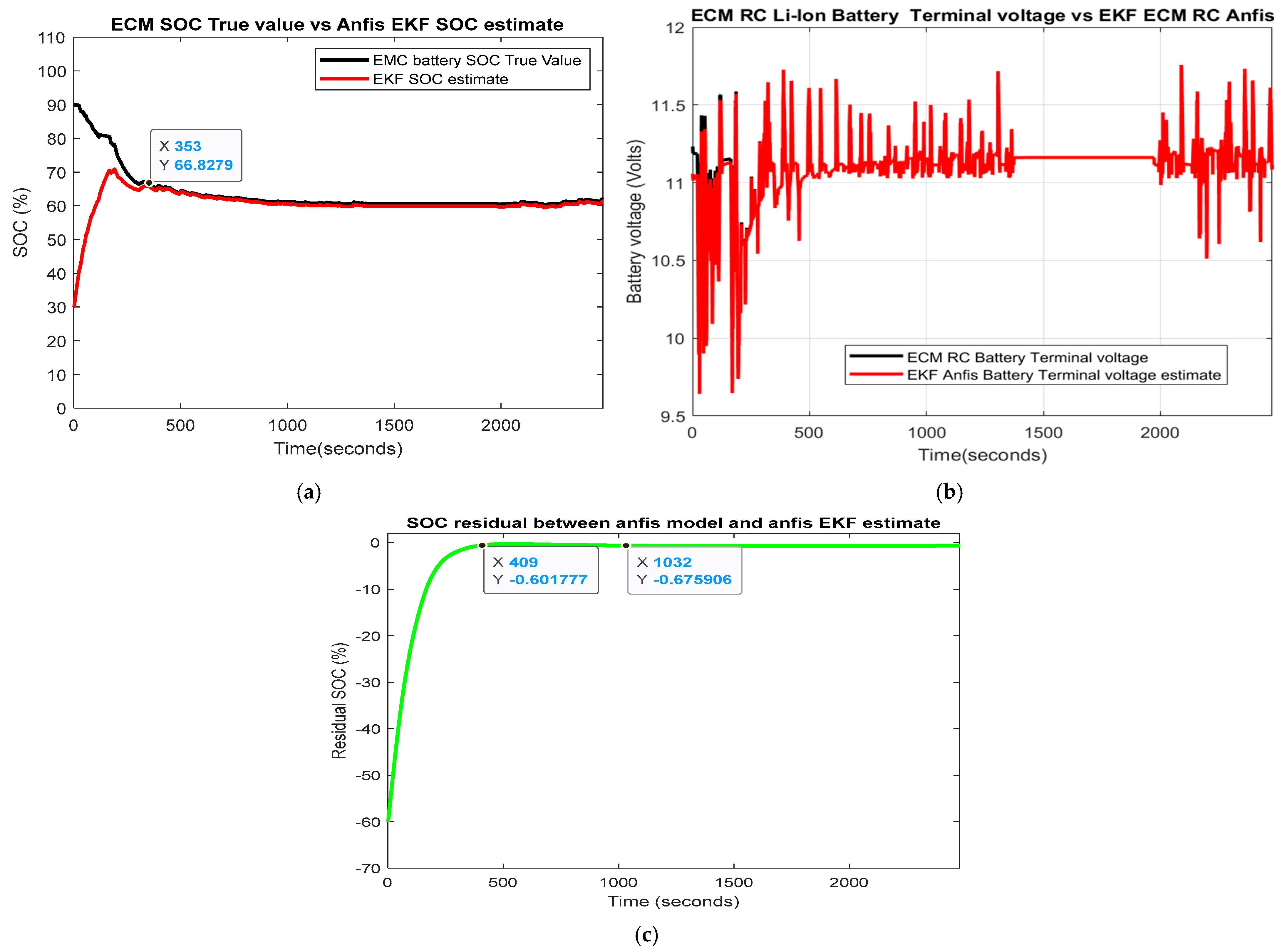
Extended Kalman filter SOC estimator design and MATLAB implementation (Section 2.5, Appendix A.1) for original and ANFIS models (Section 2.6, Figure 5, Figure 6 and Figure 7).
(d)
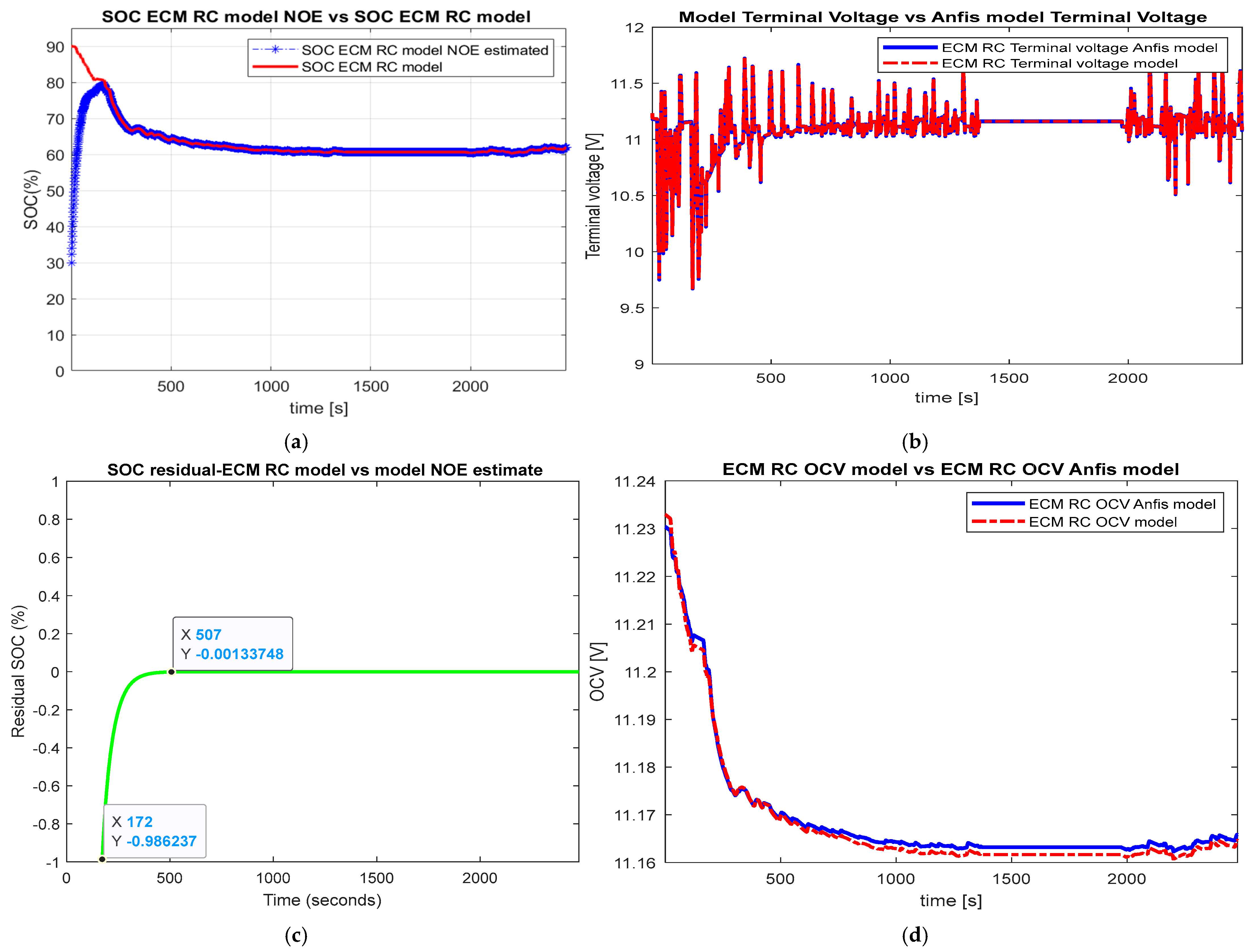
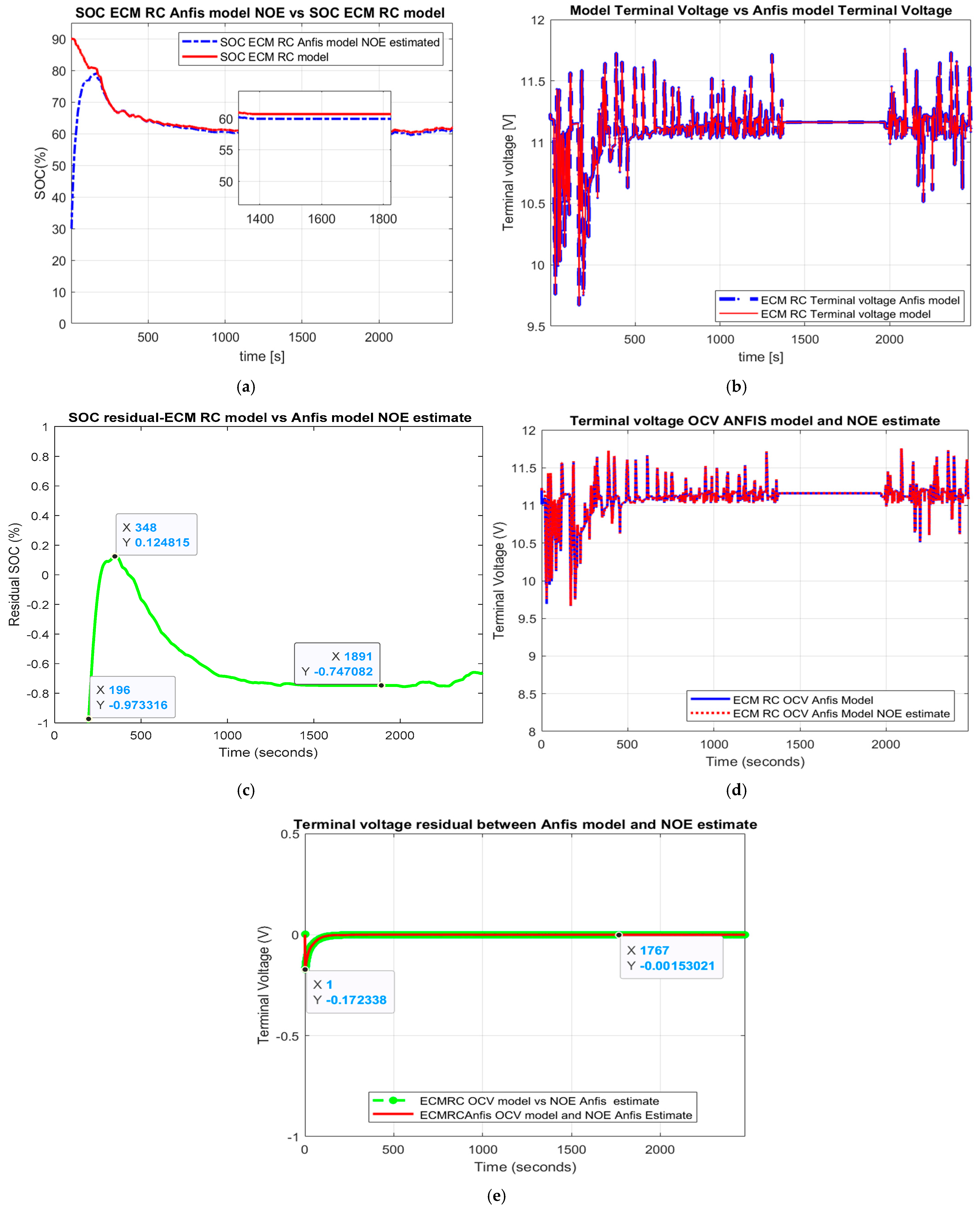
Adaptive nonlinear observer SOC (Section 2.7, Appendix B) and MATLAB SOC simulations Figure 8 and Figure 9).
(e)
Performance analysis benchmark (SOC accuracy and robustness)—Table 1 for statistical errors RMSE, MSE, and MAE. The LIB ECM RC original and ANFIS models are both of high simplicity and SOC accuracy, easy to be implemented in real-time, and provide beneficial support in building two real-time EKF and ANOE SOC estimators. The robustness and accuracy of both SOC estimators was investigated for one of the most used driving cycle tests in the automotive industry FTP-75 and changes in the SOC initial value (“guess” value) from 0.9 to 0.3. Based on the statistical errors calculated for each driving cycle test in terms of RMSE, MSE, and MAE, it was possible to choose from both traditional competitors the most suitable SOC estimator. The result of the overall performance analysis indicated that the ANOE SOC estimator for the ANFIS model performed better than the EKF SOC estimator ANFIS model.
(f)
NARX SNN LIB SOC estimator design and MATLAB implementation (Section 3.1, Figure 10) and SNN LIB terminal voltage design and MATLAB implementation.
(g)
Intelligent shallow NARX SNN SOC estimator that performs better than the traditional winner ANOE SOC estimator for the ANFIS model.
(h)
The second SNN performed better than the ANOE for the LIB terminal voltage prediction ANFIS model, with the comparison based on the MSE performance reached during the training phase.
In future works, we will continue our investigations on lithium batteries regarding an improved modelling approach by “integrating the effect of degradation, temperature and SOC effects”, and for possible extensions for more accurate ANFIS OCV(SOC) estimation techniques and new intelligent deep learning approaches.

Author Contributions

R.-E.T. contributed to algorithm conceptualization, manuscript preparation, and writing. N.T. contributed to battery model validation, performed the MATLAB simulations, and analyzed the results. M.S.R. and M.Z. contributed a formal analysis of the results, as well as to the visualization, the project supervision, and administration. H.C. contributed to manuscript preparation, corrections, visualization, and formal analysis All authors have read and agreed to the published version of the manuscript.

Funding

This research received no external funding.

Conflicts of Interest

The authors declare no conflict of interest.

Abbreviations

Li-ion Colithium-ion cobalt
EVelectric vehicle
HEVhybrid electric vehicle
BMSbattery management system
LIBlithium-ion battery
EMC RCequivalent circuit model with resistor-capacitor cell
ADVISORadvanced vehicle simulator
EPAenvironmental protection agency
UDDSurban dynamometer driving schedule.
FTP-75federal test procedure at 75 F
NEDCNew European Driving Cycle
WLTPWorldwide Harmonized Light Vehicle Test Procedure
WLTCWorldwide Harmonized Light Vehicle Test Cycles
ANOEadaptive nonlinear observer estimator
RMSEroot mean squared error
MSEmean squared error
MAEmean absolute error
OCVopen-circuit voltage
SOCstate of charge SOE state of energy
NRELNational Renewable Energy Laboratory
EKFextended Kalman filter
AIartificial intelligence
SNNshallow neural network
NARXnonlinear autoregressive with exogenous input time-series
MIMOmulti-input, multi-output systems
MISOmulti-input, single-output systems

Appendix A

Appendix A.1. Extended Kalman Filter (EKF) Algorithm—Summary Steps [11,12,13,14,15]

The LIB ECM RC is described by Equations (4)–(7), and at this point we added the process noise of 2 × 2 covariance matrix Qw, and the measurement noise of 1 × 1 covariance matrix Rv:
x k + 1 = A x k + B u k + w k
y k = C x k + D u k + h x 1 k + v k ,   D = R ,   h x 1 k = O C V x 1 k ,   x 1 k = S O C k
h x 1 k = k 0 k 1 1 x 1 k k 2 x 1 k + k 3 ln x 1 k + k 4 ln 1 x 1 k
C = d ( O C V x 1 d x 1 | x 1 k x 1 k 1  
Equation (A4) represents the components of vector C after linearization, required for the EKF algorithm, where the noises w k and v k are assumed to be Gaussian, uncorrelated, zero mean, and of covariance matrices Qw and Rv.
Steps:
  • Initialization of the states x1 (SOCini = 0.3) and x2 (Voltage polarization, x20 = 0), covariance matrix of the states Px, and tuning values for covariance matrices for the process noise Qw and measurement noise Rv.
    For k = 1, 2, 3, …, 2478 DO:
  • Prediction step
    • Prediction equations (forecast):
      x ^ ( k + 1 | k ) = A x ^ k | k + B u k + w k
      y ^ k + 1 | k = C x ^ k | k + 1 + D u k + v k
    • Prediction state covariance:
      P ^ k + 1 | k = A P ^ k | k A T + Q w
  • Correction step (measurement update)
    • Kalman filter gain computation:
      K k = P ^ k + 1 | k C T C P ^ k + 1 | k C T + R v 1
    • Correction estimates equation with a new measurement:
      x ^ ( k + 1 | k + 1 ) = A x ^ k | k + 1 + K k y m e a s u r e d y ^ k + 1 | k
    • Update the state covariance matrix:
      P ^ k + 1 | k + 1 = I 2 K k C P ^ k + 1 | k
    • Update the output estimate:
      y ^ k | k = C x ^ k | k + D u k Px = P ^ k + 1 | k + 1
END

Appendix A.2. Adaptive Neural Fuzzy Inference System (ANFIS) Model of LIB OCV(SOC) [11,18]

Step 1: Set up the training data set: LIB SOC as input, and LIB OCV as output.
Step 2: Generate the ANFIS model grid partition method-based” options”:
options = genfisOptions (‘GridPartition’)
Step 3: As one of options is to set up the number of membership functions for the fuzzy inference system (FIS):
options. NumMembershipFunctions = 5, but the user has the flexibility of increasing this number to improve the model accuracy
Step 4: Construct the FIS input attached to LIB SOC and OCV
in_fis = genfis (SOC, OCV, options)
Step 5: Select for training the OCV(SOC) ANFIS model the following options:
options = anfisOptions
options. InitialFIS = in_fis
options. EpochNumber = 20 or greater for the LIB OCV(SOC) model accuracy improvement
Step 6: Construct the FIS output attached to LIB SOC and OCV
out_fis = anfis ([SOC OCV], options)
Step 7: Plot the input–output measurement data set versus input–output OCV(SOC) ANFIS model.
plot (SOC, OCV, SO’, evalfis (SO’, ‘out_fis’))
legend (‘Training Data’, ‘ANFIS Output’).

Appendix B

Adaptive nonlinear observer estimator (ANOE) summary steps [5,11]:
  • Initialization of the states x1 (SOCini = 0.3) and x2 (voltage polarization, x20 = 0), observer filter gain L0
    For k = 1, 2, 3, …, 2478 DO:
  • NOE LIB dynamics equations
    2.1 Observer estimator gain adaptive law.
The measurements on terminal voltage of the LIB y k are generated by the LIB ECM RC model described by Equations (4)–(7).
L k = L 0 + exp β y k 1 y ^ k 1
  • NOE dynamics equations
The dynamic of LIB SOC is given by
x 1 ^ k + 1 = x 1 ^ k η T s Q n o m u k + L k y k y ^ k  
The fast dynamic for R 1 C 1 polarization voltage cell is described by
x 2 ^ k + 1 = 1 T s R 1 C 1 x 2 ^ k + T s C 1 u k
y ^ k = h x 1 ^ k + D u k  
h x 1 ^ k = k 0 k 1 1 x 1 ^ k k 2 x 1 ^ k + k 3   l n x 1 ^ k + k 4   l n 1 x 1 ^ k ,   x 1 ^ k = S O C ^ k
END

References

  1. Moshirvaziri, A. Lithium-Ion Battery Modelling for Electric Vehicles and Regenerative Cell Testing Platform. Master’s Thesis, University of Toronto, Toronto, ON, Canada, 2013. [Google Scholar]
  2. Young, K.; Wang, C.; Wang, L.Y.; Strunz, K. Electric Vehicle Battery Technologies—Chapter 2. In Electric Vehicle Integration into Modern Power Networks, 1st ed.; Garcia-Valle, R., Peças Lopes, J., Eds.; Springer: New York, NY, USA, 2013; pp. 15–26. [Google Scholar] [CrossRef]
  3. Xing, Y.; Ma, E.W.M.; Tsui, K.L.; Pecht, M. Battery Management Systems in Electric and Hybrid Vehicles. Energies 2011, 4, 1840–1857. [Google Scholar] [CrossRef]
  4. Xu, J.; Cao, B. Battery Management System for Electric Drive Vehicle-Modeling State Estimation and Balancing—Chapter 4. In New Applications of Electric Drives, 1st ed.; Chomat, M., Ed.; INTECH: Rijeka, Croatia, 2015; pp. 87–113. [Google Scholar] [CrossRef]
  5. Xia, B.; Zheng, W.; Zhang, R.; Lao, Z.; Sun, Z. A Novel Observer for Lithium-Ion Battery State of Charge Estimation in Electric Vehicles Based on a Second-Order Equivalent Circuit Model. Energies 2017, 10, 1150. [Google Scholar] [CrossRef]
  6. Cui, X.; Shen, W.; Zhang, Y.; Hu, C. A Novel Active Online State of Charge Based Balancing Approach for Lithium-Ion Battery Packs during Fast Charging Process in Electric Vehicles. Energies 2017, 10, 1766. [Google Scholar] [CrossRef]
  7. Zhang, Y.; Xiong, R.; He, H.; Shen, W. Lithium-Ion Battery Pack State of Charge and State of Energy Estimation Algorithms Using a Hardware-in-the-Loop Validation. IEEE Trans. Power Electron. 2016, 32, 4421–4431. [Google Scholar] [CrossRef]
  8. Zhang, R.; Xia, B.; Li, B.; Cao, L.; Lai, Y.; Zheng, W.; Wang, H.; Wang, W. State of the Art of Lithium-Ion Battery SOC Estimation for Electrical Vehicles. Energies 2018, 11, 1820. [Google Scholar] [CrossRef]
  9. Tudoroiu, R.-E.; Zaheeruddin, M.; Radu, S.-M.; Tudoroiu, N. Real-Time Implementation of an Extended Kalman Filter and a PI Observer for State Estimation of Rechargeable Li-Ion Batteries in Hybrid Electric Vehicle Applications—A Case Study. Batteries 2018, 4, 19. [Google Scholar] [CrossRef]
  10. Tudoroiu, R.-E.; Zaheeruddin, M.; Radu, S.-M.; Tudoroiu, N. Estimation Techniques for State of Charge in Battery Management Systems on Board of Hybrid Electric Vehicles Implemented in a Real-Time MATLAB/SIMULINK Environment. In New Trends in Electrical Vehicle Powertrains; IntechOpen: London, UK, 2019; Chapter 4. [Google Scholar] [CrossRef]
  11. Tudoroiu, R.-E.; Zaheeruddin, M.; Tudoroiu, N.; Radu, S.-M. Investigations of using an Intelligent ANFIS Modelling Approach for a Li-ion Battery in MATLAB–mplementation-Case Study. In Smart Mobility-Recent Advances, New Perspectives and Applications; IntechOpen: London, UK, 2022. [Google Scholar] [CrossRef]
  12. Farag, M. Lithium-Ion Batteries, Modeling and State of Charge Estimation. Master’s Thesis, University of Hamilton, ON, Canada, 2013. [Google Scholar]
  13. Plett, G.L. Extended Kalman filtering for battery management systems of LiPB-based HEV battery packs: Part 1. Background. J. Power Sources 2004, 134, 252–261. [Google Scholar] [CrossRef]
  14. Plett, G.L. Extended Kalman filtering for battery management systems of LiPB-based HEV battery packs: Part 2. Modeling and identification. J. Power Sources 2004, 134, 262–276. [Google Scholar] [CrossRef]
  15. Plett, G.L. Extended Kalman filtering for battery management systems of LiPB-based HEV battery packs: Part 3. State and parameter estimation. J. Power Sources 2004, 134, 277–292. [Google Scholar] [CrossRef]
  16. Tudoroiu, N.; Radu, S.M.; Tudoroiu, E.-R. Improving Nonlinear State Estimation Techniques by Hybrid Structures, 1st ed.; LAMBERT Academic Publishing: Saarbrucken, Germany, 2017; 56p, ISBN 978-3-330-04418-0. [Google Scholar]
  17. Simon, J.J.; Uhlmann, J.K. A New Extension of the Kalman Filter to Nonlinear Systems. In Process of AeroSense, Proceedings of the 11th International Symposium on Aerospace/Defense Sensing, Simulation and Controls, Orlando, FL, USA, 20–25 April 1997. [Google Scholar]
  18. Konsoulas Ilias, S. Adaptive Neuro-Fuzzy Inference Systems (ANFIS) Library for Simulink. MATLAB Central File Exchange. Available online: https://www.mathworks.com/matlabcentral/fileexchange/36098-adaptive-neuro-fuzzy-inference-systems-anfis-library-for-simulink (accessed on 19 January 2022).
  19. MathWorks MATLAB Version R2021b Online Documentation. Neuro-Adaptive Learning and ANFIS. Available online: https://www.mathworks.com/help/fuzzy/neuro-adaptive-learning-and-anfis.html (accessed on 27 March 2023).
  20. Vidal, C.; Kollmeyer, P.; Naguib, M.; Malysz, P.; Gross, O.; Emadi, A. Robust xEV Battery State-of-Charge Estimator Design Using a Feedforward Deep Neural Network. SAE Int. J. Adv. Curr. Prac. Mobil. 2020, 2, 2872–2880. [Google Scholar] [CrossRef]
  21. MathWorks MATLAB Version R2021b Online Documentation. Neuro-Fuzzy Designer. Available online: https://www.mathworks.com/help/fuzzy/neurofuzzydesigner-app.html (accessed on 27 March 2023).
  22. MathWorks MATLAB Version R2023a Online Documentation. Design Time Series NARX Feedback Neural Networks. Available online: https://www.mathworks.com/help/deeplearning/ug/design-time-series-narx-feedback-neural-networks.html (accessed on 28 March 2023).
  23. MathWorks MATLAB Version R2023a Online Documentation. Available online: https://www.mathworks.com/help/ident/ref/arx.html (accessed on 28 March 2023).
  24. Ezzeldin, R.; Hatata, A. Application of NARX neural network model for discharge prediction through lateral orifices. Alex. Eng. J. 2018, 57, 2991–2998. [Google Scholar] [CrossRef]
  25. MathWorks MATLAB Version R2023a Online Documentation. Multistep Neural Network Prediction. Available online: https://www.mathworks.com/help/deeplearning/ug/multistep-neural-network-prediction.html (accessed on 29 March 2023).
  26. MathWorks MATLAB Version R2023a Online Documentation. Fit data with a Shallow Neural Network. Available online: https://www.mathworks.com/help/deeplearning/gs/fit-data-with-a-neural-network.html (accessed on 29 March 2023).
  27. Zhang, D.; Zhong, C.; Xu, P.; Tian, Y. Deep Learning in the State of Charge Estimation for Li-Ion Batteries of Electric Vehicles: A Review. Machines 2022, 10, 912. [Google Scholar] [CrossRef]
  28. Kollmeyer, P.; Vidal, C.; Naguib, M.; Skells, M. LG 18650HG2 Li-Ion Battery Data and Example Deep Neural Network XEV SOC Estimator Script. Mendeley Data 2020, 3, 2020. [Google Scholar] [CrossRef]
  29. MathWorks Documentation. Battery State of Charge Estimation in Simulink Using Deep Learning Network. Available online: https://www.mathworks.com/help/deeplearning/ug/battery-state-of-charge-estimation-simulink-deep-learning.html (accessed on 23 April 2023).
  30. Chandran, V.; Patil, C.K.; Karthick, A.; Ganeshaperumal, D.; Rahim, R.; Ghosh, A. State of Charge Estimation of Lithium-Ion Battery for Electric Vehicles Using Machine Learning Algorithms. World Electr. Veh. J. 2021, 12, 38. [Google Scholar] [CrossRef]
  31. Johnson, V. Battery performance models in ADVISOR. J. Power Sources 2001, 110, 321–329. [Google Scholar] [CrossRef]
  32. Wipke, K.B.; Cuddy, R.M. Using an Advanced Vehicle Simulator (ADVISOR) to Guide Hybrid Vehicle Propulsion System Development; National Renewable Energy Laboratory: Golden, CO, USA, August 1996; Research Gate Net. Available online: https://www.nrel.gov/docs/legosti/fy96/21615.pdf (accessed on 1 March 2020).
  33. DieselNet-Emission Test Cycles. Worldwide Harmonized Light Vehicles Test Cycles (WLTC). Available online: https://dieselnet.com/standards/cycles/wltp.php (accessed on 22 April 2023).
  34. WLTC_class_3. Available online: https://unece.org/DAM/trans/doc/2012/wp29grpe/WLTP-DHC-12-07e.xls (accessed on 22 April 2023).
  35. Micari, S.; Foti, S.; Testa, A.; De Caro, S.; Sergi, F.; Andaloro, L.; Aloisio, D.; Leonardi, S.G.; Napoli, G. Effect of WLTP CLASS 3B Driving Cycle on Lithium-Ion Battery for Electric Vehicles. Energies 2022, 15, 6703. [Google Scholar] [CrossRef]
Figure 1. The first order Li-ion battery ECM RC schematic drawn in Multisim-14 editor.
Vehicles 05 00030 g001
Figure 2. The Simscape generic model experimental setup for Simulink simulations of a LiCO2 battery with 6.6 Ah and 11.1 V nominal voltage for possible integration into the battery pack of a HEV: (a) Experimental setup. (b) The pre-set battery setup. (c) The FTP-75 driving cycle current profile. (d) NEDC profiles tests in miles per hour (mph) and current profile in amps (A). (e) SOC Simulink generic model simulation result (focus to the interest input driving cycle current profile NDEC and Battery SOC Simscape generic model).
Vehicles 05 00030 g002aVehicles 05 00030 g002bVehicles 05 00030 g002c
Figure 3. MATLAB simulation results for the ANFIS model of nonlinear function OCV(SOC): (a) OCV ANFIS model—training phase; (b) OCV representation in time; (c) Li-ion battery SOC during a complete cycle discharge (4800 s) for a constant input current 6 A.
Vehicles 05 00030 g003
Figure 4. MATLAB simulation results for the ANFIS model of nonlinear function OCV(SOC) during a complete cycle discharge (8030 seconds): (a) SOC ANFIS model-training phase; (b) OCV ANFIS model-training phase; (c) Li-ion battery OCV(SOC) ANFIS model; (d) Li-ion battery terminal voltage during a complete cycle discharge FTP-75 repeated driving cycle current profile.
Vehicles 05 00030 g004
Figure 5. FTP-75 driving cycle current profile-MATLAB Simulink simulation results. Legend: (a) FTP-75 driving cycle current profile; (b) ECM SOC true model value versus EKF and Simscape SOC experimental extracted value; (c) SOC ECM RC value versus SOC Simscape generic model value; (d) SOC residual between the true value of the ECM RC model and the EKF SOC estimate; (e) SOC residual between the true value of the ECM RC model and the Simulink SOC experimental value; (f) ECM Li-ion battery terminal voltage at a 1 C discharging rate for a constant discharging current of 6 A during 4000 s; (g) the nonlinear OCV(SOC) Li-ion battery fitting curve at a 1 C discharging rate for a constant discharging current of 6 A for 4000 s; (h) the Li-ion battery SOC generated by ECM versus the EKF SOC estimated value generated at a 1 C discharging rate for a constant discharging current of 6 A for 4000 s.
Vehicles 05 00030 g005aVehicles 05 00030 g005b
Figure 6. MATLAB simulation results for WLTC class 3 driving cycle current profile test: (a) WLTC class 3 current profile test; (b) Li-ion ECM RC battery SOC model versus SOC Simscape model; (c) EKF ECM battery terminal voltage estimate versus the true value of the ECM model battery terminal voltage; (d) SOC residual between the SOC model and the SOC Simscape model; (e) terminal battery voltage residual between the EKF estimate and the ECM model true value; (f) Li-ion ECM RC EKF SOC estimate versus the ECM RC true value model; (g) SOC residual between the EKF estimate and the true value.
Vehicles 05 00030 g006
Figure 7. MATLAB simulation results for the NEDC driving cycle current profile test: (a) NEDC current profile test; (b) Li-ion ECM RC battery SOC model versus the SOC Simscape model; (c) EKF ECM battery terminal voltage estimate versus the true value of the ECM model battery terminal voltage; (d); SOC residual between the SOC model and the SOC Simscape model; (e) terminal battery voltage residual between the EKF estimate and the ECM model true value; (f) Li-ion ECM RC EKF SOC estimate versus the ECM RC true value model; (g) SOC residual between the EKF estimate and the true value.
Vehicles 05 00030 g007aVehicles 05 00030 g007b
Figure 8. The accuracy of the EKF ECM RC ANFIS model versus the ECM RC model: (a) OCV ECM RC model versus OCV ECM RC ANFIS model; (b) ECM RC model terminal voltage versus ECM RC ANFIS model terminal voltage; (c) ECM RC model SOC residual between the ECM RC ANFIS model and the EKF ECM RC ANFIS model.
Vehicles 05 00030 g008
Figure 9. MATLAB simulation results for the Li-ion battery NOE estimator: (a) SOC ECM RC model true value versus SOC ECM RC NOE estimate; (b) terminal voltage ECM RC model true value versus terminal voltage ECM RC NOE estimate; (c) SOC residual-ECMRC model versus model NOE estimate; (d) OCV voltage residual-ECMRC model versus ECM RC model NOE estimate.
Vehicles 05 00030 g009
Figure 10. MATLAB simulation results for the Li-ion battery OCV ANFIS model NOE estimator: (a) SOC ECM RC model true value versus SOC ECM RC OCV ANFIS NOE estimate; (b) terminal voltage ECM RC model true value versus terminal voltage ECM RC OCV ANFIS model; (c) SOC residual-ECM RC model versus ECM RC model OCV ANFIS NOE estimate; (d) terminal voltage residual-ECM RC model versus ECM RC model NOE; (e) Battery Terminal voltage model NOE estimate versus ANFIS model NOE estimate.
Vehicles 05 00030 g010
Figure 11. NARX estimator of LIB SOC estimation-neural network training phase designer.
Vehicles 05 00030 g011
Figure 12. NARX–SOC prediction MATLAB simulation results; (a) open-loop network diagram; (b) close-loop network diagram; (c) neural network–training time series response for SOC Li-ion battery ECM RC model (training phase); (d) neural network training std performances; (e) neural network regression (plot regression)-Epoch 151; (f) neural network training performance-Epoch 151; (g) neural network error autocorrelation (ploterrcorr)-Epoch 151; (h) neural network histogram (ploterrhist)-Epoch 151.
Vehicles 05 00030 g012aVehicles 05 00030 g012bVehicles 05 00030 g012c
Figure 13. Shallow neural network Li-ion battery terminal voltage estimator: (a) neural network architecture; (b) neural network training phase; (c) error histogram between target (T = yEMCanfis voltage) and output SNN estimated voltage value; (d) validation performance at Epoch 24, (e) shallow neural network estimation battery voltage value vs. battery ANFIS model voltage value; (f) the battery residual voltage between the SNN estimated voltage value and battery ANFIS model voltage value; (g) regression performance.
Vehicles 05 00030 g013aVehicles 05 00030 g013b
Table 1. Statistics for performance evaluation (SOC estimate, SOC advisor estimate, Li-Ion battery terminal voltage).
Estimates vs. ObservationsRMSEMSEMAE
SOC EKF ECM RC model vs. SOC ECM RC model0.08670.00750.0284
Terminal voltage EKF ECM model vs. terminal voltage ECM RC model0.00715.0707 × 10−57.5499 × 10⁻⁴
Terminal voltage EKF ECM model vs. terminal voltage ECM RC ANFIS model0.00725.242 × 10−50.0019
Terminal voltage NOE ECM ANFIS model vs. terminal voltage ECM RC ANFIS model0.01371.885 × 10−40.0035
SOC NOE ECM RC ANFIS model vs. SOC ECM RC ANFIS model0.05620.00310.0157
SOC ADVISOR Rint model vs. SOC ECM RC model0.06520.0040.0330
The statistics from this table reveal a very accurate LIB SOC estimation and terminal voltage prediction for LIB EMC RC for the OCV(SOC) model.
Disclaimer/Publisher’s Note: The statements, opinions and data contained in all publications are solely those of the individual author(s) and contributor(s) and not of MDPI and/or the editor(s). MDPI and/or the editor(s) disclaim responsibility for any injury to people or property resulting from any ideas, methods, instructions or products referred to in the content.

