The Vehicle Intention Recognition with Vehicle-Following Scene Based on Probabilistic Neural Networks

Abstract

In the vehicle-following scenario of autonomous driving, the change of driving style in the front vehicle will directly affect the decision on the rear vehicle. In this paper, a strategy based on a probabilistic neural network (PNN) for front vehicle intention recognition is proposed, which enables the rear vehicle to obtain the driving intention of the front vehicle without communication between the two vehicles. First, real vehicle data with different intents are collected and time—frequency domain variables are extracted. Secondly, Principal Component Analysis (PCA) is performed on the variables in order to obtain comprehensive features. Meanwhile, two cases are classified according to whether the front vehicle can transmit data to the rear vehicle. Finally, two recognition models are trained separately according to a PNN algorithm, and the two models obtained from the training are verified separately. When the front vehicle can communicate with the rear vehicle, the recognition accuracy of the corresponding PNN model reaches 96.39% (simulation validation) and 95.08% (real vehicle validation). If it cannot, the recognition accuracy of the corresponding PNN model reaches 78.18% (simulation validation) and 73.74% (real vehicle validation).

1. Introduction

Since the invention of the vehicle, there has been a never-ending quest for safety and performance. With the improvement of vehicle performance, the safety of manually driven vehicles is not guaranteed [1], but autonomous vehicles can balance safety and perform [2]. With the continuous breakthroughs in the Internet of Vehicles [3], autonomous driving is developing at a rapid pace [4]. Autonomous vehicles can improve vehicle performance compared to manual driving vehicles [5]. However, an excellent autonomous driving system requires an excellent sensing decision module [6], which needs to have the ability to accurately identify the intent of the front vehicle, thus providing the basis for planning vehicle speed, trajectory, and other decisions.

Many scholars at home and abroad have also conducted in-depth research on driving intention. For example, some scholars used a behavioral dictionary based on six typical driving behaviors to build a faster and more accurate behavioral perception model for recognition [7]. A more accurate online recognition model of a driver’s intention has been developed by using the Hidden Markov Model (HMM) [8]. In the study of emotion on driving intention, the probability distribution of driving intention under different emotions can be obtained by an immune algorithm application, so that a more realistic driving intention can be obtained [9]. At the same time, based on driving data in eight typical emotional states, the effect of emotions on driving intention conversion was obtained [10]. As time progresses, more accurate neural network algorithms are used in the scenario of driving intent recognition. Long Short-Term Memory (LSTM) neural networks recognize driving intent in real time, which is faster and more accurate than traditional back propagation neural networks [11]. Some scholars have also improved the existing driving intention model by adding Auto-regression (AR), which improves the accuracy of recognition by analyzing the driver’s previous behavior [12]. By combining multiple algorithms, some scholars have also made some results. The cascade algorithm of HMM and Support Vector Machine (SVM) are used to build the driving intention recognition model, which has greater recognition results than HMM and SVW alone and has a faster response speed [13]. Data processing is a necessary step for identification. Some scholars have studied the factor-bounded Nonnegative Matrix Factorization (NMF) problem and proposed an algorithm to ensure that the objective and matrix factors can converge, which can improve the stability of the NMF [14]. Some scholars have solved the problem of the PCA algorithm, which is sensitive to outliers and has noisy data [15].

In addition, based on the mixed traffic scenario where both autonomous vehicles and manual driving vehicles exist, a driving intention discrimination model for autonomous vehicles using HMM has been proposed, which has better recognition results in the mixed traffic scenario [16]. Based on the safety goal of reducing vehicle tailgating, a new model of safety spacing considering the rear-end braking intention has been proposed [17]. Some scholars have proposed modified safety interval strategies considering inter-vehicle braking information communication delays, brake actuator sluggishness, road conditions of each vehicle, and vehicle motion states [18]. In an autonomous driving scenario, the driving speed and optimal speed tracking controllers for autonomous vehicle formation was investigated based on the stability and integrity of predicting driving [19]. A two-layer HMM model is proposed to handle the recognition of driving intentions under combined conditions, and a maximum likelihood model is used to predict future states in the combined conditions scenario [20]. A recognition method based on improved Gustafson—Kessel cluster analysis is proposed for the driving intention of a driver’s gear change, and a corresponding fuzzy recognition system is constructed based on driving intention fuzzy rules [21]. For the recognition of driving intention during lane change, a corresponding driver lane change intention recognition model based on the Multi-dimension Gauss Hybrid Hidden Markov Model (MGHMM) was constructed and validated on Carmaker vehicle dynamics simulation software [22]. SVM-based lane change intention recognition models have also been developed by collecting corresponding driving data through driving simulators [23]. For trajectory prediction in the field of autonomous driving, a trajectory prediction model based on driving intention is proposed, which can obtain long-term prediction of future trajectory and short-term prediction of vehicle behavior [24]. Some scholars have also conducted safety studies based on curve and ramp scenarios [25,26]. There are also scholars who have achieved good results in adjusting the parameters of the torque converter based on the results of driver intent recognition [27,28].

However, most of the above research results are aimed at the driving intention recognition of autonomous driving vehicles, and less for the mixed scenarios of manual and autonomous driving. Most of the algorithms studied above have also been run only in simulation, with less consideration of real vehicle experiments. In this paper, a model of driving intention in forward vehicles that can be verified in real vehicles is proposed. When the front vehicle can transmit vehicle data to the rear vehicle, the model can carry out accurate driving intention recognition for the corresponding data. When the front vehicle cannot communicate with the rear vehicle, the rear vehicle can only measure the front vehicle speed through a sensor. As a result, the model carries out less accurate driving intention recognition. The method proposed in this paper can be a way to recognize the intention of the front vehicle without any requirement of the front vehicle. In addition, the method has good implementation implications and requires low hardware performance. The rear vehicle can base its policy on this reference value, thus improving vehicle performance while ensuring safety.

2. Research Ideas and Methods

In the vehicle-following scenario, in order to ensure a safe inter-vehicle distance, the speed change of the front vehicle will directly affect the decision judgment of the rear vehicle. When the front vehicle accelerates, the rear vehicle can choose to accelerate appropriately according to its own vehicle status, thus improving the fuel economy and power of the vehicle. In this paper, we mainly consider the performance of the vehicle in the vehicle-following scenario, so we mainly recognize the acceleration intention of the front vehicle, and when the rear vehicle recognizes the acceleration intention of the front vehicle, it can reduce the safe inter-vehicle distance appropriately to improve the economy and power of the vehicle.

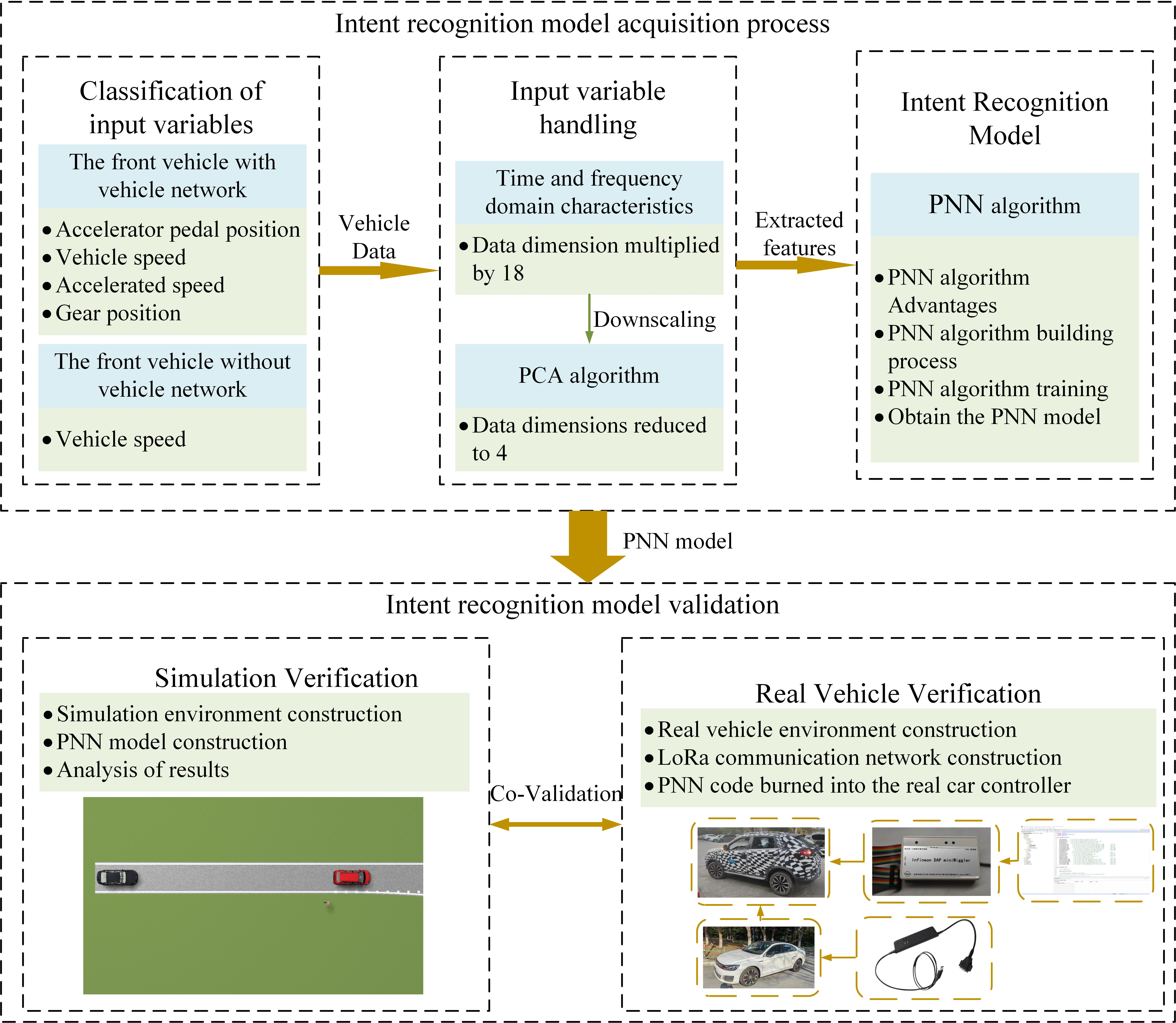
In the vehicle-following scenario, the driver’s intention is directly reflected in the operation of the accelerator pedal, and the vehicle speed, gear and acceleration can also reflect the driver’s intention, so this paper chooses the accelerator pedal position, speed, acceleration, and gear position information as the original input of the data. These data need to be sent from the front vehicle to the rear vehicle. If the front vehicle cannot transmit this data, the rear vehicle can collect the speed of the front vehicle through the sensor, but the accuracy of the recognition result will be slightly worse than the former. Therefore, in this paper, the model is trained in the same way for two cases, one with four inputs and the other with one input. The workflow of model training is shown in Figure 1. The driver data can be collected from the driver model in the simulation environment or from the driver driving a real vehicle. There is a certain difference between the driving behavior of the driver model in the simulation environment and the real driver, so this paper uses existing equipment such as Kvaser to collect vehicle status information through CAN communication. There are four types of working conditions collected, which are mild, normal, less aggressive, and aggressive. The data for these four intents were collected by professional drivers driving on the road with the accelerator pedal open at around 10%, 20%, 30%, and 50%. The lengths of the data sets are 120,739, 111,010, 111,413, and 33,954, respectively. Due to the small variety of the original data, a time domain analysis is performed in this paper in order to make the eigenvalues of each driving intention as distinguishable as possible. After time domain analysis processing, many time domain features of the data can be obtained, which can make different driving intentions have more distinguishing features, thus making the recognition results more accurate. However, too many features will slow down the recognition speed; we need to ensure the accuracy while minimizing the computing time, so this paper adopts the PCA to extract the integrated feature values. The processed data will be used as samples to start training the model. For the real vehicle experiment, the PNN model, which is easy to implement in hardware, is chosen in this paper.

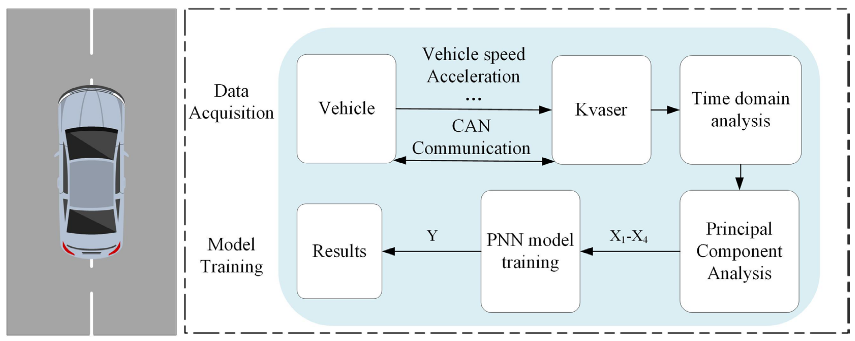
The verification idea of the simulation and the real vehicle test is the same, as shown in Figure 2. In the vehicle-following scenario, after collecting vehicle data via Kvaser, the front vehicle transmits the data to the rear vehicle via the Internet of Vehicles. As mentioned earlier, there are two types of data collected by the front vehicle, one includes speed, gear, accelerator pedal position, and acceleration signal, and the other is speed signal only. The raw data obtained in both cases need to be processed in the time—frequency domain and the PCA. The processed data are used as the input to the trained PNN model, and the final output results are compared with the actual results. In this paper, simulation and real vehicle experiments are conducted for both cases.

In addition, after the data are acquired, they need to be pre-processed in advance. The useless data between different intents and data that do not conform to common sense are deleted. The pre-processed data are divided into training and test sets with a ratio of 8:2. The training set is first used for PNN training, and then the test set is used to validate the model obtained from the training. After that, two scenarios are verified in a real vehicle environment according to whether the front vehicle can communicate or not. In this paper, different experimental vehicles and different testers were used in order to ensure the accuracy of the test results as much as possible.

3. Time Domain Analysis Processing and PCA Dimensionality Reduction

In the actual driving of the vehicle, it is not reasonable to judge driving intentions by the state of the vehicle in the moment. It is normal for different driving intentions to have the same speed and other vehicle status in the moment. Therefore, this paper adopts the sliding window intercepts data as the input of the model. The meaning of the sliding window is that as time increases, new data is gradually added and old data is gradually deleted, with the length of the window always being a constant. With this approach, recognition results can be outputted at any time and the accuracy of the recognition results can be guaranteed. The length of the window is the amount of data, and in terms of the amount of data selected, if the amount of data selected is too small, the features of the data will not be obvious enough, thus leading to inaccurate recognition results, and if the amount of data selected is too large, it will lead to untimely output results. Therefore, in a comprehensive comparison, this paper chooses to use 3000 data for processing, and the sampling time of the data is 0.001 s. That is, each intent recognition decision will be based on the last three seconds of data.

In order to make full use of the data and improve the recognition accuracy, it is necessary to process the data. In this paper, we mainly process the data in the time domain, extracting the time domain features of the data segments, such as mean value, root mean square value, etc. As shown in

Table 1. Feature meaning.

No.	Meaning	No.	Meaning
1	Maximum value	10	Skewness
2	Minimum value	11	Rms amplitude
3	Average value	12	Form factor
4	Peak-to-peak value	13	Crest factor
5	Absolute mean	14	Impulse factor
6	Root mean square (Rms)	15	Clearance factor
7	Variance	16	Spectral center of gravity
8	Standard deviation	17	Rms frequency
9	kurtosis	18	Frequency variance

, a total of 18 features were extracted. However, the time domain processed data will bring too much computation, which will lead to a too long recognition time and is not conducive to hardware implementation. Therefore, the simulation time needs to be reduced as much as possible while maintaining the recognition accuracy. There are more kinds of methods for dimensionality reduction, among which PCA dimensionality reduction is mainly covariance matrix calculation, and the calculation process is not complicated and easy to implement in hardware. In this paper, we use the PCA for dimensionality reduction, which is an unsupervised dimensionality reduction method. The main idea is that if we want to reduce 6-dimensional data to 3-dimensional, we need to find 3 orthogonal features and make the maximum variance of the data after mapping; the larger the variance, the bigger the dispersion between data points and the greater the degree of differentiation. The main effect of PCA is to reduce the simulation time, and it is not based on the association with the labels, but on the variance to classify the principal components. The variance is calculated as shown in Equation (1).

$${\sigma }_x^2=\frac{1}{n}{\displaystyle {\displaystyle \sum _{i=1}^n}{(x_i-\bar{x})}^2},$$

(1)

For the simplicity of the calculation, it is necessary to make the mean of each data zero before the formal dimensionality reduction. This operation does not change the distribution of the sample, but only corresponds to a translation of the coordinate axes. Thus, the formula for calculating the variance is shown in Equation (2).

$${\sigma }_x^2=\frac{1}{n}{\displaystyle {\displaystyle \sum _{i=1}^n}{x}_i^2},$$

(2)

The variance is the deviation of the data from a feature before dimensionality reduction, while the covariance is used to determine whether the new feature will affect the original feature. Therefore, in addition to calculating the variance, PCA dimensionality reduction also requires the calculation of the covariance, and the calculation of the covariance of the feature X and the feature Y is calculated as follows.

$$Cov(X,Y)=\frac{1}{n}{\displaystyle {\displaystyle \sum _{i=1}^n}{x}_i}{y}_i,$$

(3)

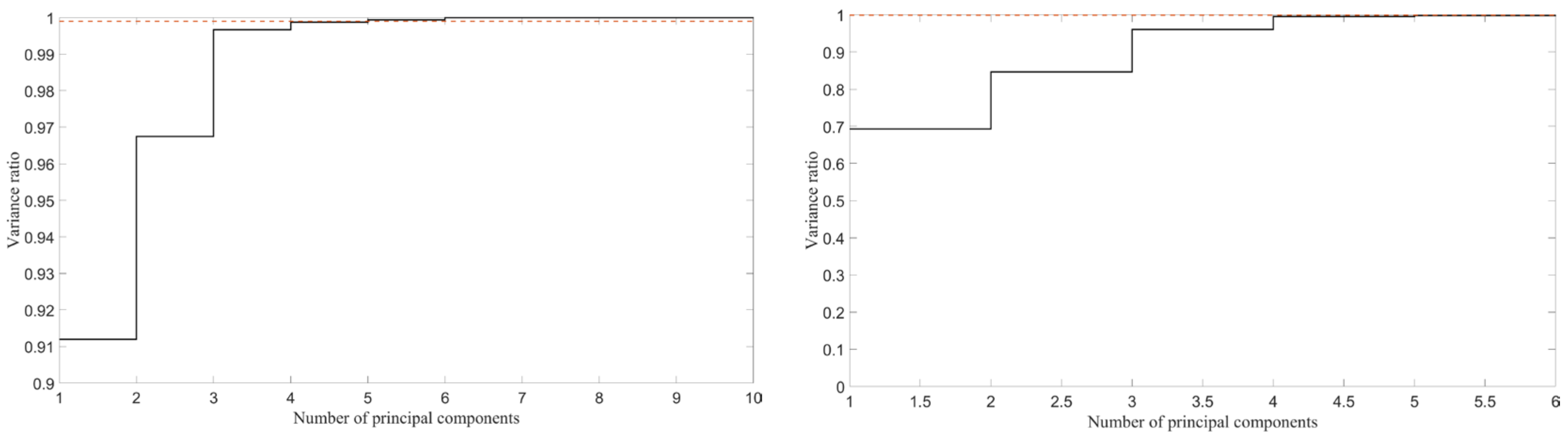
In the calculation process, the eigenvectors of the covariance matrix are the principal components, and their corresponding eigenvalues are the variances of the principal components. The larger the eigenvalue corresponding to this eigenvector in the covariance matrix, the larger the variance represents, and the more obvious the differentiation of the data mapped to this eigenvalue, so it is more appropriate to choose him as the principal component. Therefore, the size of the eigenvalue can be used to determine which principal component direction contains the size of the data, so that the final number of principal components can be determined. As shown in Figure 3, the number of principal components selected in this paper is 4, and the final data volume that can be included is 99.87% (one input variable) and 99.58% (four input variables). The n-th variance ratio in the figure is calculated as the ratio of the sum of the variances of the first n principal components to all principal components.

In this paper, Matlab software is used to write the relevant algorithms, and the final result is a transformation matrix, and the transformed data principal components are obtained by multiplying the data with this matrix. The transformed data are used for subsequent model design and training. When the PCA is not used, the input data has a total of 18 dimensions (one input variable) and 72 dimensions (four input variables) and when the PCA is used, the input data has 4 dimensions. Therefore, this approach greatly reduces the simulation time.

4. PNN Algorithm

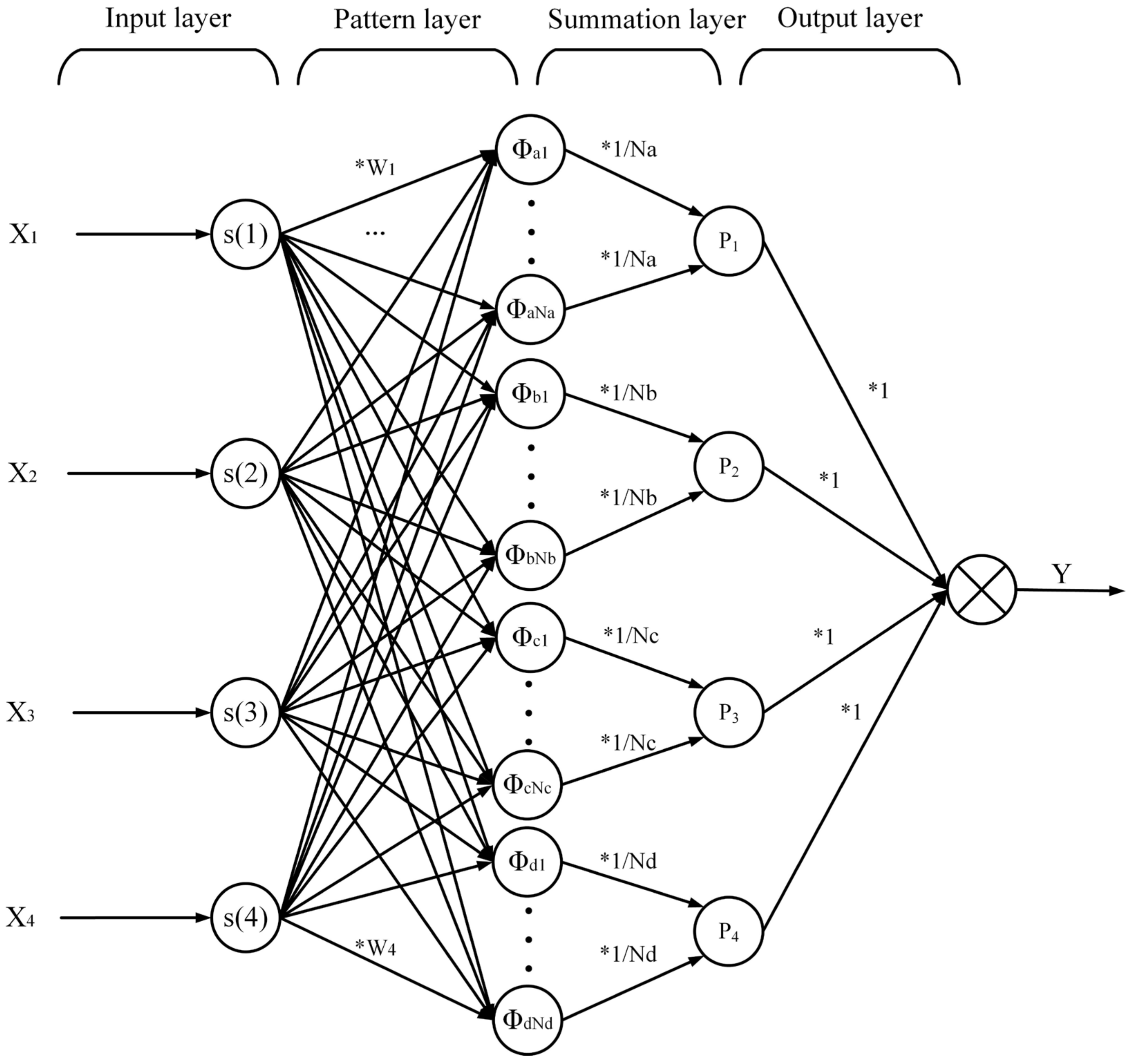
The PNN algorithm consists of a combination of an input layer, a pattern layer, a summation layer, and an output layer, and its structure is shown in Figure 4. The PNN algorithm is based on radial basis neural networks and uses Bayesian decision rules as the basis for classification, which has the following advantages:

• Easy training and fast convergence make PNN classification algorithms ideal for real-time processing;
• The pattern layer uses a radial basis nonlinear mapping function, so the PNN can converge to a Bayesian classifier as long as sufficient sample data are available;
• The transfer function of the pattern layer can be chosen from various basis functions used to estimate the probability density with better classification results;
• The number of neurons in each layer is relatively fixed and thus easy to implement in hardware.

From the results of PCA, it can be seen that there is a total of four inputs to the PNN algorithm used in this paper, as shown in X₁–X₄. The input layer does not perform computation, but simply transforms the input data into vector s and passes it to the neurons in the pattern layer. The pattern layer is a radial base layer, and the function chosen in this paper is a Gaussian function. In the actual calculation, the vector s in the input layer needs to be multiplied with the weighting coefficients, as shown in ‘*W₁’ in the figure. The selection of PNN weights relies on the size of the feature value corresponding to each feature in the PCA dimensionality reduction. The larger the eigenvalue of a feature, the more data it contains and the more important it is. The formula for calculating the initial weight is the variance of the feature divided by the sum of the variances of all features. After that, the weights change as the model is trained. There are four types Φ_a–Φ_d of pattern layer, corresponding to four classification results, where the output of the n-th neuron is shown in Equation (4).

$${\Phi }_{\mathrm{n}}\left(\mathrm{s}\right)={\mathrm{e}}^{-\frac{(s-w_n){(s-w_n)}^T}{2{\alpha }^2}},$$

(4)

where ${\Phi }_{\mathrm{n}}\left(\mathrm{s}\right)$—The output of the n-th pattern layer neuron;

$\alpha$—Smoothing factor;

$s$—The vectors corresponding to the model inputs;

$w_n$—The weight vector of the n-th pattern layer neuron.

The summation layer does a weighted average of the output of the pattern layer, and each summation layer neuron represents a category. In total, this paper collects the recognition results under four driving intentions, which are mild, normal, less aggressive, and aggressive. There are four neurons in the summation layer, and the output of the i-th neuron is shown in Equation (5).

$$P_i=\frac{1}{L}{\displaystyle {\displaystyle \sum _{n=1}^L}{\Phi }_{i,n}(s)},$$

(5)

where $P_i$—Weighted output of the i-th category;

$L$—Number of pattern layer neurons pointing to the i-th category;

${\Phi }_{i,n}(s)$—The output of the n-th pattern layer neuron pointing to the i-th category.

The output layer follows the Bayesian decision rule to decide the final output class. The minimum risk decision is the general form of Bayesian decision making, when the risk function is shown in Equation (6):

$$P_R(c_i\left|s\right.)={\displaystyle {\displaystyle \sum _{h=1}^4}{\lambda }_{i,h}{P}_h(c_h\left|s)\right.},$$

(6)

where $P_R(c_i\left|s\right.)$—The risk when the input vector is judged to be the i-th category;

${\lambda }_{i,h}$—Losses when judging category h as the i-th category;

$P_h(c_h\left|s)\right.$—The conditional probability of the input vector when judged into the h-th category the output of the PNN model in a comparison of the input with the trained data, the probability of similarity is calculated. ${\lambda }_{i,h}$ represents the loss when wrong results are outputted. This value can be increased appropriately when the output of the wrong result has little impact. In this paper, due to the safety of the vehicle involved, ${\lambda }_{i,h}$ is set to 1 when the correct result is outputted, and 0 otherwise. Then equation 6 is updated to Equation (7).

$$P_R(c_i\left|s\right.)=1-P_h(c_i\left|s\right.),$$

(7)

Therefore, in order to minimize $P_R(c_i\left|s\right.)$, then $P_h(c_i\left|s)\right.$ is maximum. So that is, the output layer takes the class corresponding to the output of the maximum summation layer.

5. Algorithm Validation and Real Vehicle Experiment

In this paper, both simulation and real vehicle experiments are used for validation. The purpose of the simulation is to verify the accuracy of the recognition. The purpose of the real vehicle experiments is to verify the generality of the results and to verify the ease of implementation of the recognition algorithm.

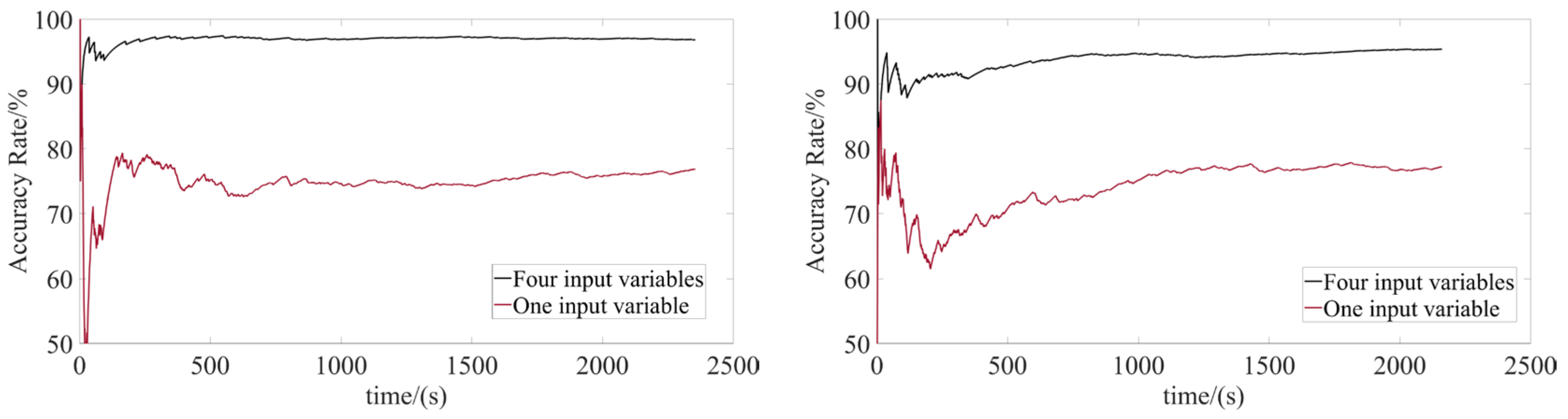
In this paper, we used Prescan and Simulink for joint simulation verification, where Prescan provided the road environment and Simulink controlled the vehicle operation. The vehicle model was built based on the demo file of Prescan. In the simulation environment, there were two vehicles driving in the same direction on a road. The front vehicle drove with different driving intentions and the rear vehicle performed recognition. The rear vehicle recognized the driving intention of the front vehicle based on the information received. The result of the recognition is shown in Figure 5 and Figure 6. The horizontal coordinates in the figure represent time, and each recognition is made using the last 3 s of data. The vertical coordinate in the figure is the recognition accuracy rate. As time increases, the accuracy rate changes continuously, and the final average accuracy rate is 96.39%. where accuracy rate is defined as follows:

$$Acc=\frac{TP}{TP+FP},$$

(8)

where $Acc$ accuracy rate of recognition;

$TP,FP$ are the number of samples with correct and incorrect identification results, respectively.

When the front vehicle is unable to transmit status information, the rear vehicle can only judge the intention by the speed of the front vehicle. In this paper, the final average accuracy rate of knowing only the speed information of the front vehicle was 78.18%.

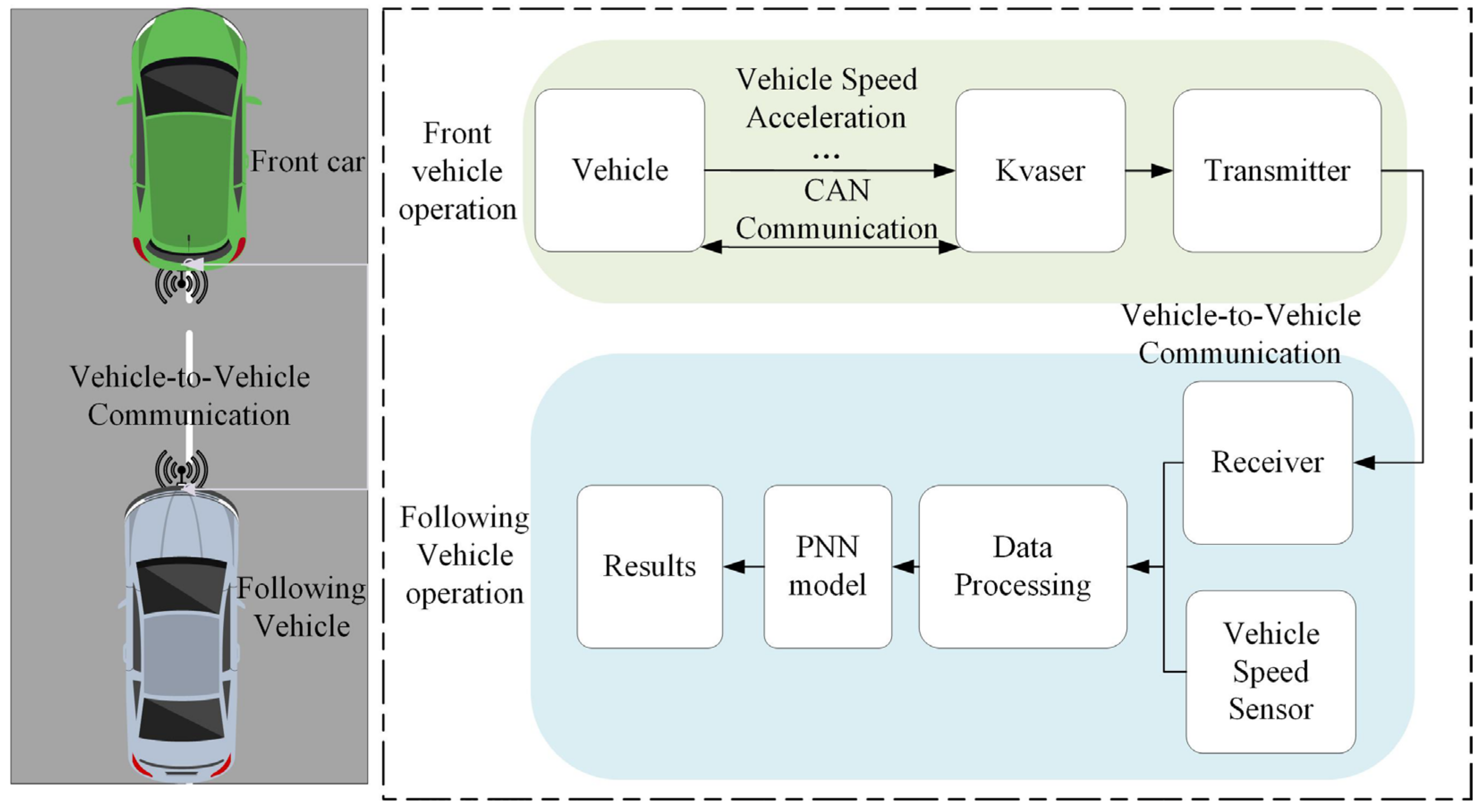
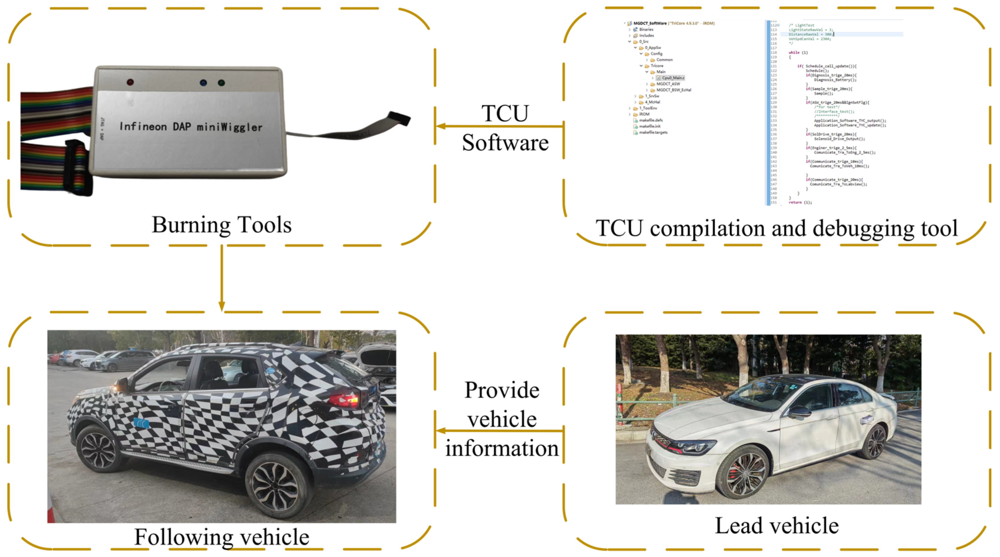
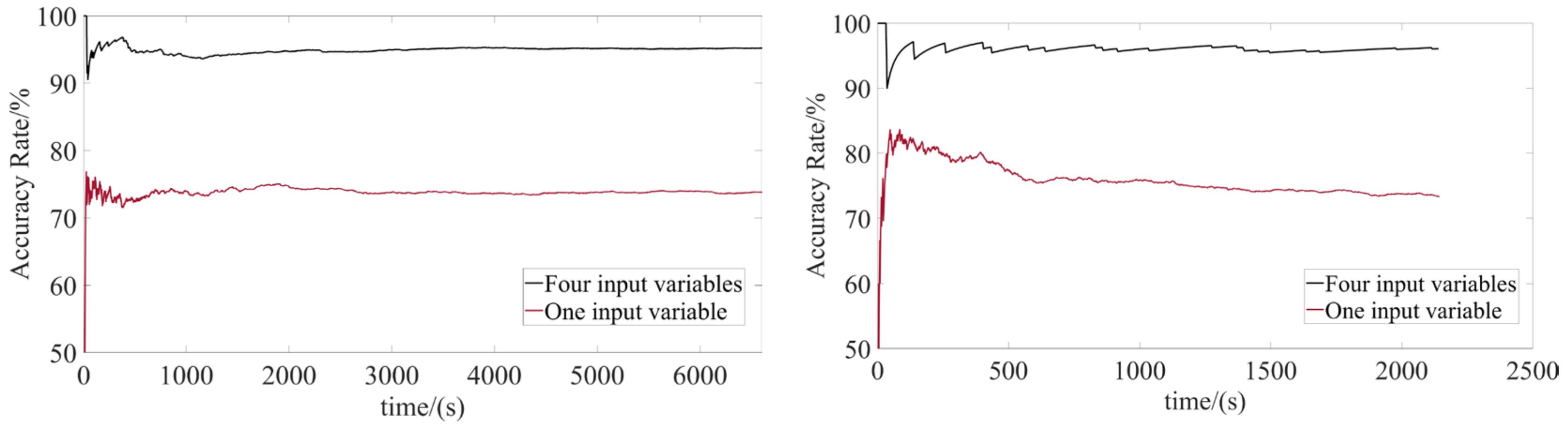
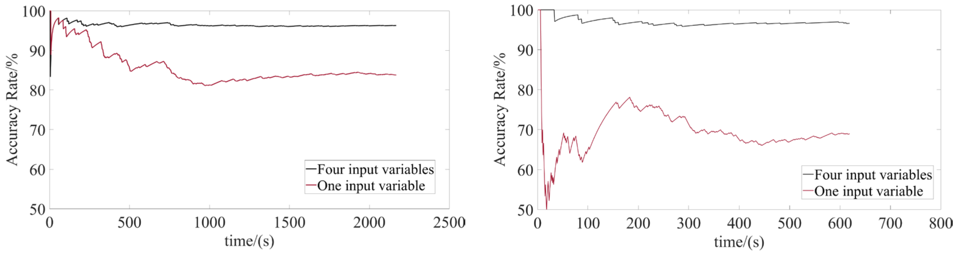
In the real vehicle experiment, as shown in Figure 7, two vehicles are used in this paper. The front vehicle collects data through the Kvaser device and sends it to the rear vehicle through a LoRa chip. The rear vehicle receives the data and sends it to the transmission control unit (TCU) through the UART serial port. The PNN model is burned into the TCU for recognition. In this paper, experiments were conducted according to two cases, one was to send four vehicle status information and the other was to send only vehicle speed information. As shown in Figure 8, the recognition average result in the first case was 95.08%.

Due to the safety considerations during driving, only the first two intentions were experimented in this paper. As can be seen from the figure, the accuracy rate was steady as time increased, which means that the recognition algorithm does not recognize only a certain situation but has a similar ability to recognize most situations. The recognition accuracy decreased when the rear vehicle could only obtain the speed information of the vehicle in front, and the final average recognition result was 73.74%.

In summary, as shown in

Table 2. Recognition results.

Work Conditions		Correct Rate $\left(\mathit{A}\mathit{c}\mathit{c}\right)$	Variance of the Correct Rate $\left({\mathit{\sigma }}_{\mathit{A}\mathit{c}\mathit{c}}^2\right)$	Peak-to-Peak of the Correct Rate $\left({\mathit{\sigma }}_{\mathit{A}\mathit{c}\mathit{c}}^2\right)$
Simulation (with four input variables)	mild	96.81%	0.88	3.45
	normal	95.37%	3.30	7.55
	less aggressive	96.31%	0.44	2.21
	aggressive	96.60%	0.83	2.16
Simulation (with one input variable)	mild	76.90%	9.33	9.39
	normal	77.18%	18.33	16.43
	less aggressive	83.80%	17.48	14.96
	aggressive	68.98%	29.16	13.14
Real vehicle (with four input variables)	mild	95.05%	0.19	3.26
	normal	95.93%	0.49	1.57
Real vehicle (with one input variable)	mild	73.84%	4.11	4.64
	normal	73.37%	13.13	9.18

, the recognition model proposed in this paper has good performance in both simulation and real vehicles. The recognition accuracy was around 95% when more information about the front vehicle could be obtained, and around 73% when only speed information about the front vehicle could be obtained. The vehicle could carry out corresponding measures to improve the vehicle performance according to the recognition results of the front vehicle. The variance of the accuracy could reflect the suitability of the algorithm. The lower variance of the recognition accuracy indicates that the algorithm has a similar recognition ability for various working conditions. The peak-to-peak value is the maximum value minus the minimum value in a segment of data, which can reflect the sharpness of the curve. Since the sample size is too small at the beginning of identification, the accuracy at this time is not meaningful and this part of the data is not included in the calculation of peak-to-peak values. The final calculation results are shown in Table 2.

6. Summary and Prospect

This paper focuses on the recognition of acceleration driving intentions of the rear vehicle to the front vehicle in a vehicle-following scenario. The purpose of this work was to enable the rear vehicle to take countermeasures in advance according to the change of the front vehicle’s intention in an autonomous driving scenario, so that a greater vehicle performance could be obtained while ensuring safety. In this paper, we also considered the driving intention recognition when there was no Internet of Vehicle. By processing and analyzing the vehicle driving data, it was possible to provide the rear vehicle with a reference value of the driving intention of the front vehicle in most cases. The specific work is as follows:

• This paper identified the research idea. The idea of identification is to analyze and process the existing data, determine the driving behavior characteristics, and build a model using a PNN algorithm.
• The data were processed in the time domain and processed by the PCA. By combining time domain analysis and PCA, the main features of the data were extracted, redundant data calculations were avoided, and the computation was effectively reduced on the basis of accuracy, thus laying the foundation for real vehicle experiments;
• The processed data were trained by the PNN algorithm, which had the advantage that the number of neurons is fixed, thus making the implementation of the algorithm simpler. In addition, the PNN model was simpler to train, which further reduced the amount of computation required for recognition.
• In this paper, the PNN model was verified by both simulation and the real vehicle. The validation of simulation is mainly to ensure the accuracy of the model, and the validation of the real vehicle is mainly to ensure the generalizability of the model. This paper also validated the model based on the situation when there is no vehicle network and achieves good results.

Through the above series of work, this paper verifies the feasibility of recognizing the driving intention of the front vehicle. However, this paper only studied the vehicle-following scene, and did not expand it to a variety of scenarios. The subsequent research will gradually consider more scenarios, such as signal light scenarios. In addition, during the research process of this paper, many algorithms with excellent performance were therefore excluded due to the consideration of real vehicle experiments. Later, more advanced algorithms can be used to further improve the accuracy of recognition by upgrading the vehicle controller.