Article

Computational Analyses of the Effects of Wind Tunnel Ground Simulation and Blockage Ratio on the Aerodynamic Prediction of Flow over a Passenger Vehicle

1
NC Motorsports and Automotive Research Center, UNC Charlotte, Charlotte, NC 28223, USA
2
Chip Ganassi Racing Team, 8500 Westmoreland Dr NW, Concord, NC 28027, USA
3
AXISCADES Engineering Technologies Ltd., 3008 W Willow Knolls Dr, Peoria, IL 61614, USA
*
Author to whom correspondence should be addressed.
Vehicles 2020, 2(2), 318-341; https://doi.org/10.3390/vehicles2020018
Submission received: 18 May 2020 / Revised: 2 June 2020 / Accepted: 5 June 2020 / Published: 11 June 2020

Abstract

:
With the fast-paced growth of computational horsepower and its affordability, computational fluid dynamics (CFD) has been rapidly evolving as a popular and effective tool for aerodynamic design and analysis in the automotive industry. In the real world, a road vehicle is subject to varying wind and operating conditions that affect its aerodynamic characteristics, and are difficult to reproduce in a traditional wind tunnel. CFD has the potential of becoming a cost-effective way of achieving this, through the application of different boundary conditions. Additionally, one can view wind tunnel testing, be it a fixed-floor or rolling road tunnel, as a physical simulation of actual on-road driving. The use of on-road track testing, and static-floor, and rolling-road wind tunnel measurements are common practices in industry. Subsequently, we investigated the influences of these test conditions and the related boundary conditions on the predictions of the aerodynamic characteristics of the flow field around a vehicle using CFD. A detailed full-scale model of Hyundai Veloster with two vehicle configurations, one with the original and the other with an improved spoiler, were tested using a commercial CFD code STAR-CCM+ from Siemens. Both vehicle configurations were simulated using four different test conditions, providing overall eight different sets of simulation settings. The CFD methodology was validated with experimental data from the Hyundai Aero-acoustic Wind Tunnel (HAWT), by accurately reproducing the test section with static floor boundary conditions. In order to investigate the effect of the blockage ratio on the aerodynamic predictions, the vehicle models were then tested with moving ground plus rotating wheel boundary conditions, using a total of four virtual wind tunnel configurations, with tunnel solid blockage ratios ranging from 1.25%, which corresponds to the actual HAWT, to 0.04%, which presents an open air driving condition.

Graphical Abstract

1. Introduction

As one of the three major source of road vehicle energy losses, besides the power train losses and vehicle mass [1], aerodynamic drag reduction remains the one of the major focuses of interest for both race and road vehicle industries over the last few decades. To minimize exhaust emissions, and improve the fuel efficiency and handling characteristics, automotive manufacture focuses on the aerodynamic drag reduction starting from the early stages of vehicle design. Wind tunnel testing, road testing, and CFD simulations are the three common tools used by the industry to evaluate the aerodynamic performance of a vehicle. However, during the early design and optimization stages, road testing cannot be applied, since a complete car has not been manufactured. Thus, manufacturers can only rely on wind tunnel testing and CFD simulation to improve the design.
Automotive wind tunnels are designed to simulate the on-road vehicle performance with a physical vehicle model placed in bounded test sections. Wind tunnel test sections are categorized as closed wall, open jet, slotted wall, and adaptive wall; however, none of these can accurately reproduce the actual on-road aerodynamic performance of the vehicle [2]. Subsequently, correction factors must be applied to wind tunnel test results, to account for the restrictions in the testing conditions, such as the effects of wind tunnel solid blockage and other boundary corrections.
Wind tunnel test section interference effects on ground vehicle aerodynamic testing have been investigated for decades. Both experimental and numerical studies have sought to quantify and correct the interference effects on the tested vehicle model caused by differences in the test section configuration and size. Since closed wall and open jet configurations are the two most commonly used test section configurations, a vast majority of the research works concentrated primarily on these two designs.
Studies on the wind tunnel interferences were first reported by Glauert [3] when he introduced a blockage correction to measurements on aircraft wings and bodies carried out in a closed wall test section. Cooper [4] and his co-workers pioneered the automotive related studies with his complete view on “closed-test-section wind tunnel blockage correction for road vehicles”. Later, Mercker and Wiedemann [5] suggested four other interference effects evident in open jet tunnels, all of which are related to the changes of static pressure along the streamwise direction in the test section.
Research works on the open jet and closed wall wind tunnels were carried over by Mercker’s team and others into the new century as well [5,6]. Wickern [7] had his first summary on the application of automotive wind tunnel corrections, followed by Wickern and Schwartekopp [8], who investigated the nozzle gradient effects in open jet wind tunnels. Hoffman et al. [9,10] studied the test section configuration effects on the aerodynamic drag and lift predictions as well, with different vehicle shapes using the Ford/Sverdrop Drivability Test Facility. Based on experiments carried out using various vehicle models, Mercker and his co-workers were able to quantify the effects of the static pressure gradients in wind tunnels [11]. They proposed two-measurement correction methods [12], which are currently widely used in the industry for aerodynamics prediction corrections for both experiments [13] and CFD simulations [14,15].
Even though CFD capabilities have greatly been improved with the rapid growth of computational power, showing much better correlation with wind tunnel measurements, the latter is still considered the favored reference, due to the real physical models and real air-flow conditions [16]. CFD simulations, however, can provide a much deeper insight into the flow field interacting with the vehicle [17,18], and can be a very effective tool during the design optimization process [19]. Researchers have demonstrated the capabilities of CFD in delivering valuable aerodynamic predictions, and even replicating the wind tunnel tests with certain mesh resolutions, boundary conditions, and physical modeling. By taking the Jaguar Land Rover program as an example, Gaylard [20] emphasized that a good combination of simulation and wind tunnel testing can provide more competitive aerodynamic performance than relying fully on either methodology. Similarly, Ueno et al. [21] reported a good agreement between the CFD simulation results and wind tunnel measurements with an error margin of ±5% for their open-wheel race car study. Most recently, the Hyundai Motor Company used a quarter-scale Genesis model to investigate the reproduction of wind tunnel tests with CFD simulations [22].
Two major challenges of replicating wind tunnel tests in CFD are, firstly, correctly simulating the different types of ground configurations in the test section and secondly, the implementation of the upstream boundary conditions. Many numerical studies have been carried out on these topics as well. Wickern et al. [23] from AUDI AG studied the boundary layer suction effects on vehicle drag, and illustrated the importance of a suction or boundary layer control system. Buscariolo and Mariani [24] investigated the influence of three types of ground, viz. the static floor, elevated plate, and moving belt, using a small pickup truck model in 2D simulations. Hennig et al. [25] used CFD to evaluate measurement interference effects of various Rolling Road Systems (RRS), which include single belt, 3-belt, 5-belt, and T-belt systems. Most recently, Meederira et al. [26] presented CFD analyses characterizing the wake flow structures past an isolated wheel and its interaction with a 5-belt moving ground plane (MVP).
Simulating the rolling-road system requires accurate modeling of the wheel rotation as well. In fact, the drag results coming from the configuration with only moving ground and no wheel rotation are higher, when compared to the static floor and fixed-wheel conditions; with both moving ground and wheel rotation active, the drag prediction will be lower [27]. The effects of the moving ground plane (MVP) and rotating wheel (RW) systems have been studied both experimentally and computationally during the last two decades. Research in this area covered isolated wheels, to cite but a few [26,28], and vehicle models with both simplified wheels [29] and detailed wheels [27,30]. More recently, several CFD works [27,31,32] have focused on investigating the MVG-RW influence on vehicle aerodynamic predictions using PowerFLOW, a Lattice Boltzmann based CFD approach. In these studies, different wheel rotation methods were applied, which include rotating boundary conditions, moving reference frames (MRF), and sliding mesh.
Although a significant number of works have been published concerning CFD and wind tunnel correlations [33,34,35,36,37,38,39,40], very few of these studies investigated the comparison among wind tunnel tests with both static floor, rolling-road, and track testing from a numerical investigation point of view. A numerical comparison between different wind tunnel test sections, viz. open jet, slotted wall, and adaptive wall and a blockage free tunnel, was presented by Connor et al. [41]. The blockage free domain was designed to simulate conditions equivalent to the road testing. All the simulations were run with the rolling-road system. Moreover, the focuses on the interference effect of open jet test sections suggested that having different vehicle models or mounting the same model at different longitudinal locations caused pressure gradient and wake changes. Not many researchers investigated the influence of the test section volume on the prediction results, since the open jet test section itself is less sensitive to the blockage effects compared to the closed wall section.
In the present study, a detailed full-scale model of Hyundai Veloster was tested using CFD under both wind tunnel and interference free conditions. The simulations were validated using the experimental results from the Hyundai Aero-acoustic Wind Tunnel (HAWT) in Namyang, South Korea. Both static floor with fixed wheels and moving ground with rotating wheels were modeled in both domains to evaluate ground simulation effects. To capture the open jet test section interference effects on the vehicle model, the virtual test section was scaled up by 225% and 400% of the original CAD (Computer-Aided Design) model. The static pressure distribution for each scale was studied in the streamwise direction. Changes of the vehicle drag coefficient caused by different pressure gradients were indicated and explained. In addition, a modified rear spoiler was designed during the study and its performance is assessed against the baseline vehicle model using wind tunnels with MVP and no-MVP. As a matter of fact, the discrepancy observed between the CFD and HAWT wind tunnel predicted performance gain is the primary reason of undertaking the studies presented in this paper.

2. Wind Tunnels and Boundary Conditions

Two types of computational domains were modeled in the study, with both static and moving floor cases in each model. Firstly, the Hyundai Aero-acoustic Wind Tunnel (HAWT) at Namyang Technical Center was simulated by accurately reproducing its three-quarter semi-open jet test section, using information available in the literature. The purpose of reproducing HAWT is to validate the CFD methodology with the static floor test data from that tunnel. The blockage effect of the open jet test section was evaluated by scaling the wind tunnel model in width and height to 1.5 and 2.0 times its original dimensions, but keeping the same length, which resulted in 225% and 400% of the actual HAWT test section in volume, respectively. Secondly, for the road-testing simulations, a nearly interference-free domain (blockage ratio of 0.04%) was built to eliminate the blockage effect, where the CFD predictions are more comparable to the real vehicle performance. As mentioned before, two spoiler geometries were tested in all four domains, and the results will be discussed in the following sections.

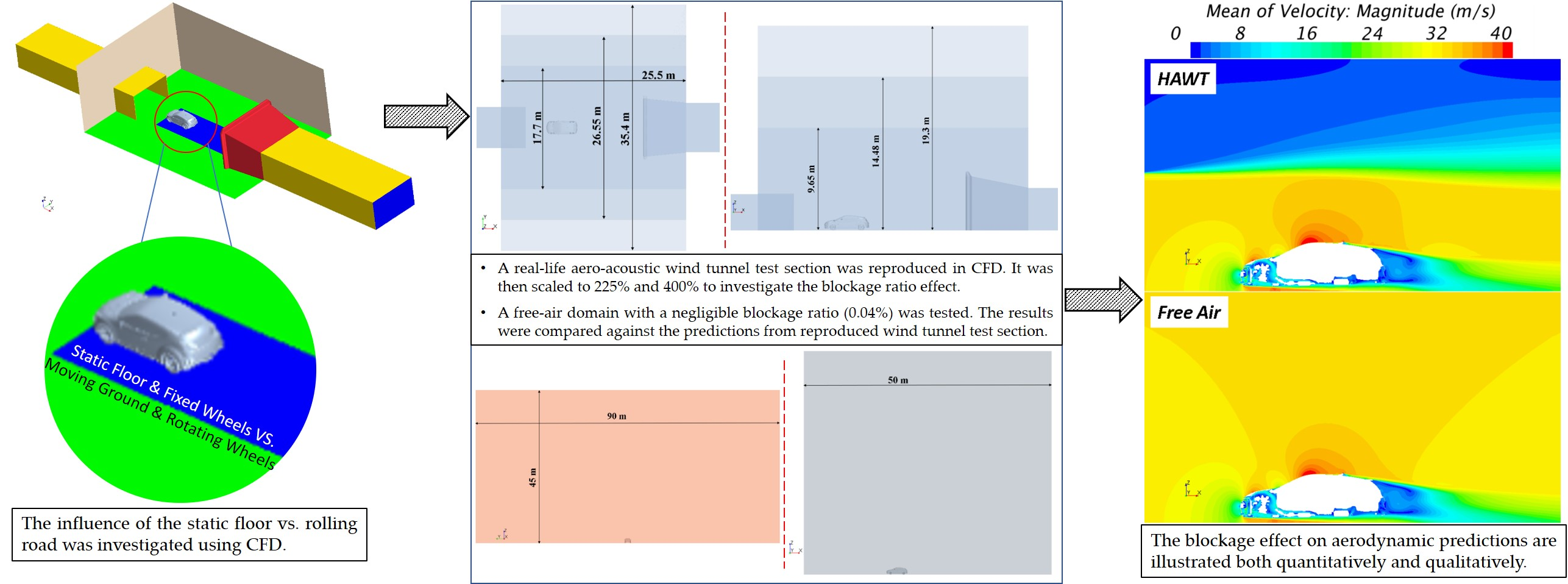
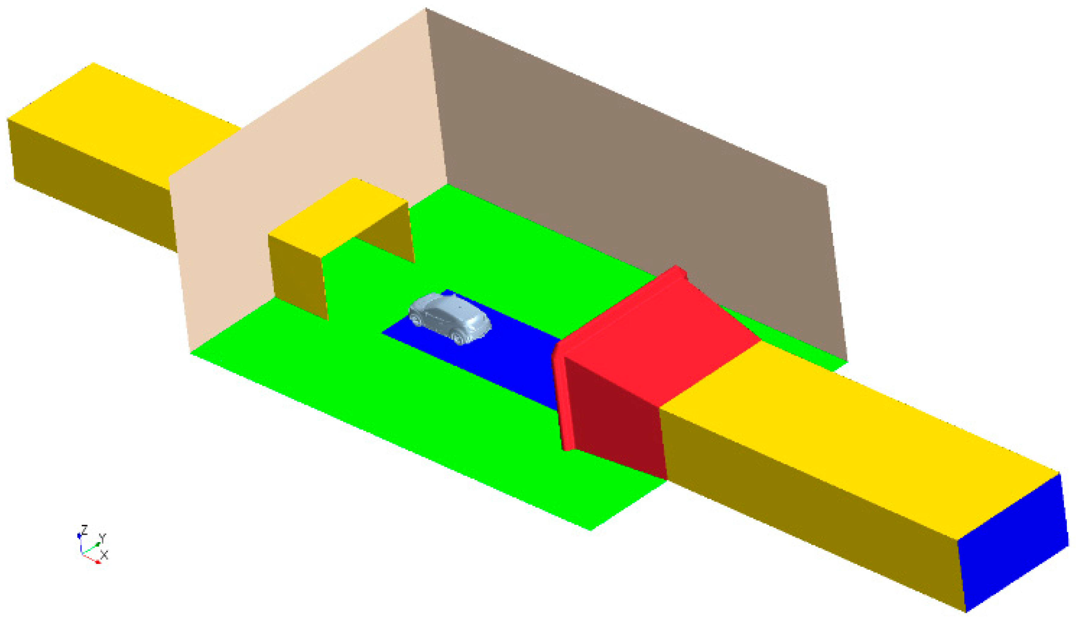
2.1. Hyundai Aero-Acoustic Wind Tunnel (HAWT) Model

The Hyundai Aero-acoustic Wind Tunnel, HAWT for short, is a full-scale, closed circuit, open jet working-section wind tunnel designed for carrying out aerodynamic, aero-acoustic, and engine cooling related tests [42]. HAWT has a test section 25.5 m long, 17.7 m wide, 9.65 m high, and a nozzle outlet measuring 28 m2; this corresponds to a wind tunnel solid blockage ratio of 1.25% for the tested vehicle model, 2014 Hyundai Veloster. Interested readers are referred to Kim et al. [42] for more details of the HAWT design methodologies, layout, instrumentations, flow controls, and visuals, which includes photographs of the critical sections and top and side views of the test section. A CAD model of the HAWT tunnel was created using the information available in [42], and is shown in Figure 1. This CAD model includes a simplified flow inlet, an outlet diffuser, and a moving-belt system under the vehicle. The nozzle contraction for the inlet was not included in the model, because it has little impact on the flow in the test section [15,43].
In order to investigate the effects of the test section volume on the prediction of aerodynamic characteristics of the test vehicle, the computational test section was inflated in horizontal ( Y ) and vertical ( Z ) directions to reach expanded test section volumes, which are 225% and 400% of the actual test section volume. Figure 2 represents top and side views of the scaled-up test sections. These two inflations of the test section in vertical and spanwise directions resulted in the wind tunnel solid blockage ratios of 0.56% and 0.30%, respectively, for the tested vehicle.

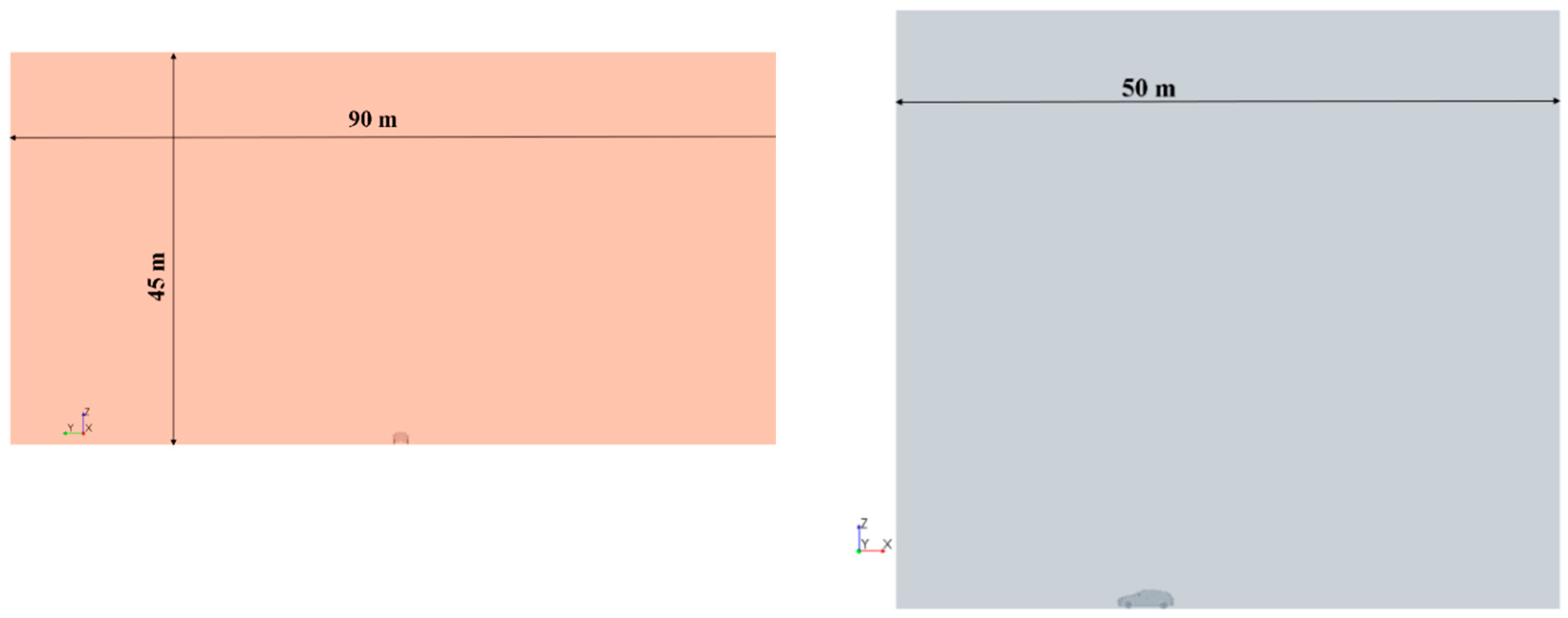
2.2. Blockage-Free Domain

The blockage free domain, which is a rectangular box, has a negligible blockage ratio of 0.04%; therefore, the model can be considered as placed in free air simulating road testing conditions for the vehicle. The domain extends 12-car length (50 m) in X , 21-car lengths (90 m) in Y , and 10.5-car lengths (45 m) in Z , as shown in Figure 3. The boundary conditions on the ground plane of this free air tunnel is the same as the MVP version of the HAWT tunnel. That is an area on the floor around the vehicle is designated as a moving ground, which has a no-slip boundary condition with a tangential velocity equal to the free-stream velocity assigned to it, while the rest of the ground plane is treated as slip-wall for computational efficiency. The two side walls and the roof of the domain were also set to as slip walls, to avoid any possible effects from the growth of boundary layers over these boundaries.

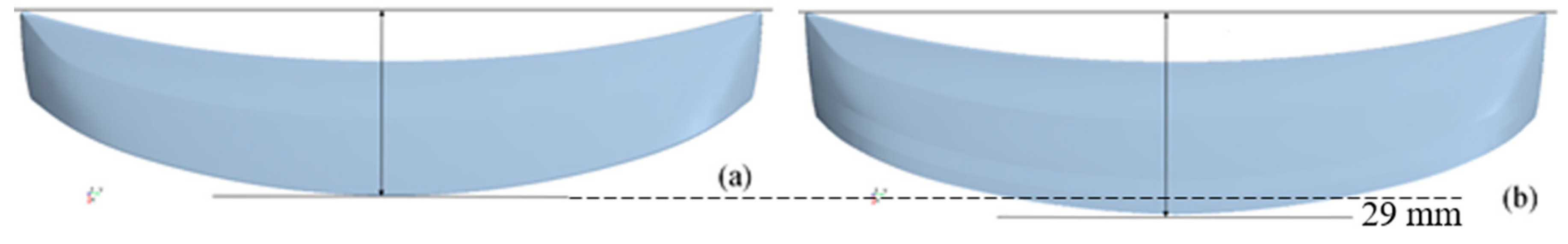
2.3. Spoiler Geometries

One purpose of this study is to verify the performance increase of the redesigned spoiler in terms of drag reduction, compared to the original spoiler. In order to reduce the vehicle drag and lift, the redesigned spoiler was extended by 29 mm in chord length (Figure 4), and featured a smoother trailing edge. The new spoiler also features a smoother transition from the roof, to positively impact the flow resistance at that point, as shown in Figure 5.
Both spoilers were tested in the HAWT test section and free air environment, with both static and moving floor boundary conditions. The comparisons showed a consistent improvement for the drag with the redesigned spoiler.

3. Numerical Setup

3.1. HAWT Model

The CFD model was meshed using the trimmer mesh; prism layer mesh was activated to better capture the boundary layers along the no-slip boundaries. As seen in Figure 6, higher mesh density was applied to the regions surrounding the vehicle and its wake, to capture the areas of high flow gradients. The underbody mesh was sufficiently refined to capture the ground effect. The shear layer development and the possible flow recirculation at the nozzle exit were also accounted for with a relatively dense mesh. The total cell number for the HAWT model configuration with the full-scale Veloster was about 70 million.

3.2. Blockage-Free Model

The mesh around the vehicle for the free air condition was identical to the mesh used in the HAWT model case, including the wake and underbody treatments. To control the cell number in this big domain within the bounds of existing computational power, five levels of volumetric control sources were used to restrain the fine regions. The cell size decreases from 384 mm to 24 mm (from the region marked as “5” to the region marked as “1”), as listed in Table 1 and shown in Figure 7.

3.3. Spoiler Mesh

As a more accurate prediction of the spoiler performance was critical to this study, the flow surrounding the spoiler needed to be predicted with a sufficient level of accuracy. As such, the region surrounding the spoiler was resolved, with a very fine mesh of 6 mm to minimize the numerical error accumulation; our preliminary studies showed that going below this mesh size does not affect the results at all. This mesh scheme for the spoiler is shown in Figure 8.

3.4. Initial and Boundary Conditions

A velocity inlet boundary condition was applied to the domain upstream with a constant uniformed incoming flow of 31.293 m/s or 70 mph and a turbulence intensity of 0.5% to match the wind tunnel test conditions. A pressure outlet boundary condition is used at the domain outlet. The moving ground effect was achieved by applying a tangential velocity, the same as the air speed, to the no-slip floor patch under the vehicle. The tire rotation in this case was simulated by a constant tire rotation rate.

3.5. Turbulence Model

The simulations were carried out using a commercial CFD code, STAR-CCM+ by Siemens, using a steady-state Reynolds-Averaged Navier-Stokes (RANS) solver. The two turbulence models tested during the study which include the Realizable k ε (RKE) [44] and Shear Stress Transport k ω (SST) [45] models. The k ε turbulence model solves for the turbulent kinetic energy ( k ) and kinetic energy dissipation rate ( ε ). The RKE model is an improvement over the standard k ε model, as it features a different formulation for the turbulence viscosity, and a new transport equation for the dissipation rate. Instead of a constant C μ , the RKE model uses a variable C μ to make the model to be more compatible. The existing literature suggests that the SST model predicts both free-stream flows and boundary layers all the way down to the viscous sub-layer with good accuracy; however, it usually predicts larger turbulence levels when compared to the the k ε model.
Preliminary investigations with the models show that he RKE and SST models over-predicted the vehicle drag coefficient by 10 and 22 counts, respectively, compared to the test data from HAWT. This small three to five percent over-prediction of drag may come from two reasons. Firstly, our CFD replication of the HAWT may not be exact, and we might have missed some flow control of the HAWT. Secondly, the RANS simulations of the unsteady flow around a vehicle are far from perfect. In consideration of these two facts, the CFD results seems to be well within the acceptable level of accuracy, which adds a reasonable confidence in the of the CFD results presented in this paper. Since the RKE results better correlate with the wind tunnel data, with less than 3% of difference in drag prediction, it was chosen as the turbulence model for further investigations.
The transport equations for turbulent kinetic energy k , and the dissipation rate ε , for the RKE model are given by
k t + U j k x j = τ i j U i x j ε + x j [ ( ν + ν t σ k ) k x j ] ,
k t + U j k x j = C 1 ε k τ i j U i x j C 2 ε 2 k + ν ε + x j [ ( ν + ν t σ ε ) ε x j ] ,
ν t = C μ k 2 ε
C μ = 1 A 0 + A s κ U * ε
where   A 0 = 4.04 , A s = 6 cos ϕ , ϕ = 1 3 cos 1 6 W , W = ( S i j S j i S k i ) / S ˜ and S ˜ = S i j S j i , where S i j is the mean rate of train tensor.

3.6. Solver and Convergence

The simulations were carried out with a segregated solver. A 2nd order discretization was used for the source and diffusion terms, and a 2nd order upwind scheme for the convection terms of the momentum equations. Each simulation took 4000 iterations to converge. The oscillations of drag and lift coefficient values of the vehicle were within 0.5% during the last 1000 iterations, and the reported mean drag coefficient C D and lift coefficient C L were calculated by averaging the values over last 500 iterations.

4. Results and Discussion

Several cross-sections were created around the vehicle to analyze the flow-filed around it which are shown in Figure 9. To facilitate the subsequent discussion these cross sections are labels with numbers 1–7, the list below shows the location and plane-type of each of these sections.
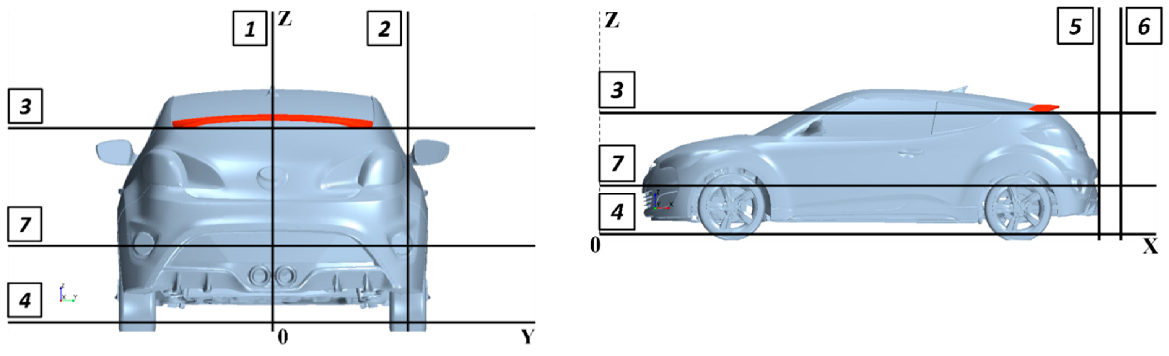
  • XZ-plane along the vehicle center line at Y = 0;
  • XZ-plane through the right-tire center at Y = 0.78 m;
  • XY-plane thru the spoiler at Z = 1.17 m;
  • XY-plane near the ground at Z = 0.05 m;
  • YZ-plane at the rear fascia at X = 3.4 m, wake cross-Section 1;
  • YZ-plane at X = 3.6 m, wake cross-Section 2;
  • XY-plane observing jet expansion at Z = 0.47 m.

4.1. Wind Tunnel Boundary Interference Effects

The simulation results of the detailed full-scale model of Veloster was validated in the virtual HAWT test section with the test data from HAWT. Table 2 shows the CFD and wind tunnel correlation results. HAWT data are proprietary and confidential. As such, all results presented in this paper were normalized by an arbitrary frontal area, to match the drag coefficients seen in open domain published resources.
The discrepancies between the CFD prediction and wind tunnel result are consistent for both spoilers. If the reported drag coefficient value from wind tunnel is the measured data without any interference correction, the numerical model over-predicted the vehicle drag by 3% (10 counts); however, because of the lack of details about the HAWT test procedure, the authors cannot guarantee if the reported data had been corrected. Despite that, an attempt has been made to correct the CFD predicted drag value thus obtained using a simplified wind tunnel interference correction procedure. An interested reader is referred to a recent publication by Cooper et al. [46], for details of why boundary corrections are a standard practice for the open-jet wind tunnel testing of automobiles.
The current literature is rich with various methods proposed for wind tunnel interference effect corrections. Some of these procedures are rather simple, and some are very sophisticated and require multi-point measurements. This paper attempts to apply wind tunnel interference corrections to the uncorrected CFD data, using one of these simple methods, as outlined below.
The correction methodology used in this paper is a twostep process. This process starts with first applying the solid blockage correction to the uncorrected C D   measurements to account for wind tunnel test section solid blockage restriction. The next step is to apply the buoyancy corrections to this first = order corrected drag to account for the higher-order wall interference induced variation of pressure gradient along the vehicle centerline.
Per Katz [2], one of the simplest solid blockage corrections can be formulated as:
C d B = C d u   1 ( 1 + 1 4 · A C ) 2   ,
where C d u is the uncorrected drag coefficient, C d B is the corrected C D   after blockage correction, A is the model front area, and C is the cross-sectional area of the open jet test section. The correction method proposed by Mercker and his co-workers [11,12] was then applied to the solid-blockage corrected drag coefficient C d B . This procedure, as outlined below, corrects measurement errors induced due to the wake distortion caused by the pressure gradient over the vehicle wake [12]. The corrected drag coefficient ( C d c ), after considering of the wake distortion and horizontal buoyancy corrections, can be written as:
C d c = [ C d B ( ± C p D ) ] n
C p D = C p W + C D H B
C p W = C P w c C P m b
where n = q c / q u is the dynamic pressure correction factor, C D H B is the horizontal buoyancy correction term, q c denotes the corrected dynamic pressure of the wind tunnel stream, and qu is the measured dynamic pressure, C P m b and C P w c are the pressure coefficients in the empty tunnel at the base of the vehicle model and at the location of wake closure, respectively.
C D H B = G ( V m S f ) ( d C p d x )
where V m is the model volume and d C p d x denotes the static pressure gradient. The Glauert factor [47] G is defined as:
G = ( 1 + 0.4 t L )
where L is the model length, and the model thickness t is given by t = 2 2 S f π , where S f is model frontal area. An interested reader is referred to Mercker et al. [12] for further details.
When the corrections detailed above are applied to the CFD calculations, the corrected CFD predicted C d of the original spoiler case becomes 0.329, which shows only 0.5% discrepancy when compared to the wind tunnel data. Without further verification from the experiment, it is hard to claim that the CFD predicted the vehicle drag accurately; however, the fact that the CFD result is close to the corrected wind tunnel test data gives some confidence in the numerical settings for the CFD model.

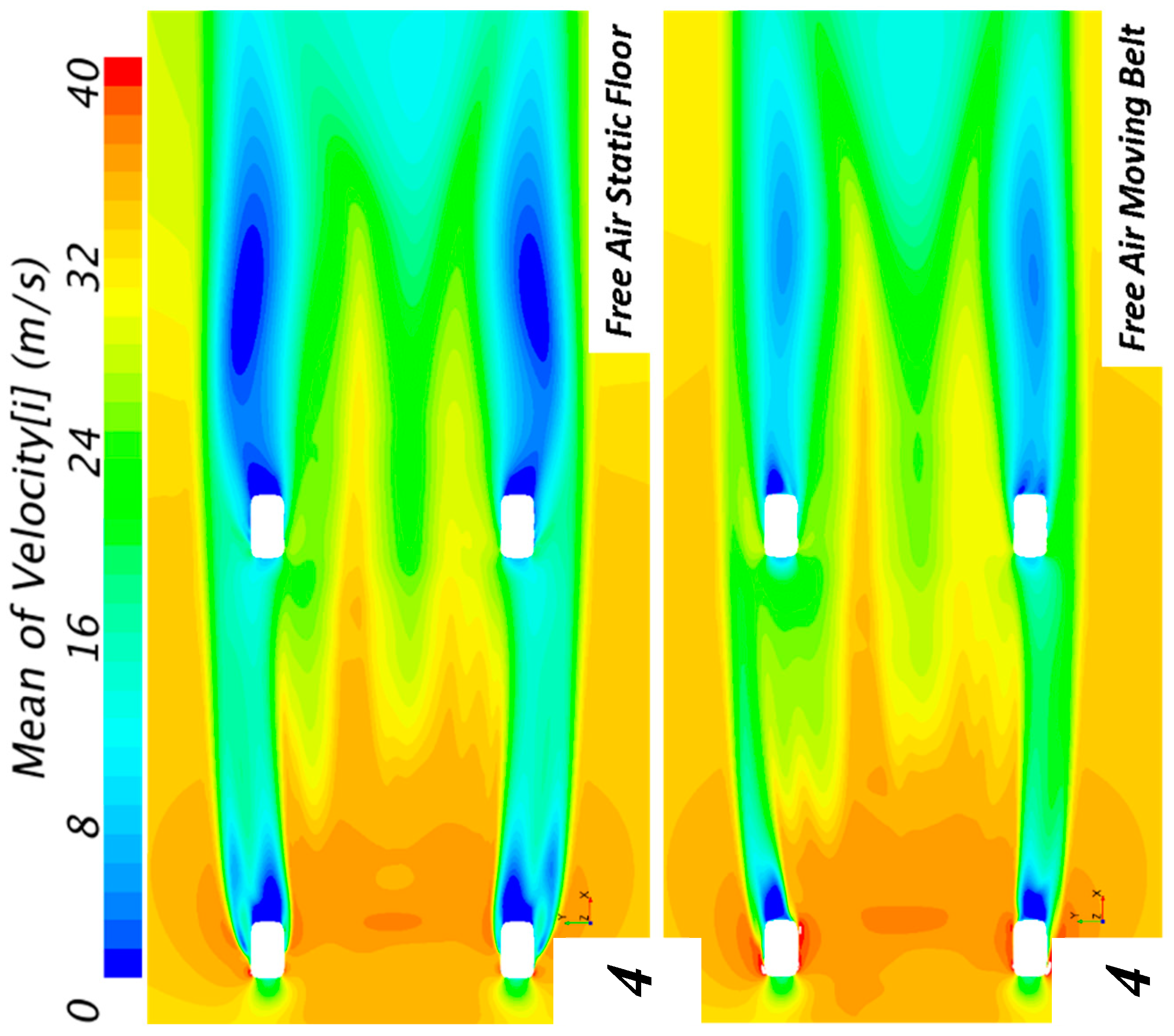
4.2. Static and Moving Ground Effects

The static and moving ground planes in the wind tunnel were simulated in CFD using two different boundary conditions. For fixed ground and fixed wheels (FG&FW) simulations, the physics conditions for tires, wheels, and ground were set to be static walls. Denser prism layers were applied to the frictional ground to capture the boundary layer development, similar to [26].
For the moving ground and rotating wheels (MVG&RW) simulations, two common methods of wheel rotation are (1) moving reference frame (MRF) and (2) local rotation rate. To avoid numerical artifacts arising from the geometry complexity near the wheels, a local rotation rate boundary condition was applied to all rotating boundaries, including the tires, wheel frames, wheel hubs, and brake rotors. Since the four wheels of the Hyundai Veloster model have the same radius, they were all set to a rotation rate of 100.1 rad/s. A moving-ground boundary condition was also applied to the no-slip floor at the same speed of the incoming flow (70 mph or 31.393 m/s).
A comparison between the drag coefficients obtained from the static and moving floor CFD simulations, with the vehicle model placed inside HAWT, can be seen in Table 3. For both the original and improved spoiler cases, the delta C D between the static floor and moving ground simulations is 5 counts. In other words, the moving ground boundary condition simply translated the Veloster performance line vertically down by 5 counts. This trend agrees with the work done by Waschle [48] on the influence of rotating wheels on the vehicle’s aerodynamics characteristics obtained using a detailed Mercedes E class model, where a reduction of 12 counts of drag was reported when changing from static to moving ground. Waschle [48] stated that the change in drag due to the rotating wheels and moving ground is mainly caused by the change of underbody flow and rear tire wakes.
Figure 10 compares the streamwise mean velocity on a Z-plane at Z = 0.05 (plane 4) obtained from the static floor and moving ground CFD simulations with the vehicle model placed inside the HAWT. The velocity contours show a marked difference between the cases in the wake region behind the tires. For the static floor case, both front and rear tires generated much stronger wakes compared to the moving ground case, especially for the rear tires. This is in line with the findings of Waschle [48], and is the main reason why the static floor CFD simulations show a higher drag for the same vehicle configuration. The change in the front tire wakes can be identified more clearly on the side view analysis, as shown in Figure 11. It is noticeable that the wake has a shorter streamwise extent for the moving ground case.
A similar phenomenon was observed too in the CFD simulations with the vehicle model placed in the blockage free domain, labelled as the free air environment, as presented in Figure 12 and Figure 13. The rotating tires and moving ground significantly reduced the wake behind the tires (Figure 12), which indicates higher velocity flow under the vehicle. From the side view of the velocity magnitude scalar image in Figure 13, the increase of velocity is obvious with the expansion of high velocity contour area. The change of the velocity profile under the car also leads to a lift change, the MVG&RW system in the simulations caused a decrease in vehicle lift for both domains. Table 4 presents the drag and lift coefficient delta between the static and moving ground boundary condition cases; the data presented correspond to the vehicle model with the original spoiler mounted. Although no reported lift coefficient values were available from the wind-tunnel test to validate the lift prediction, the reduction in lift for the free air case is close to what Waschle [48] has reported in his work.

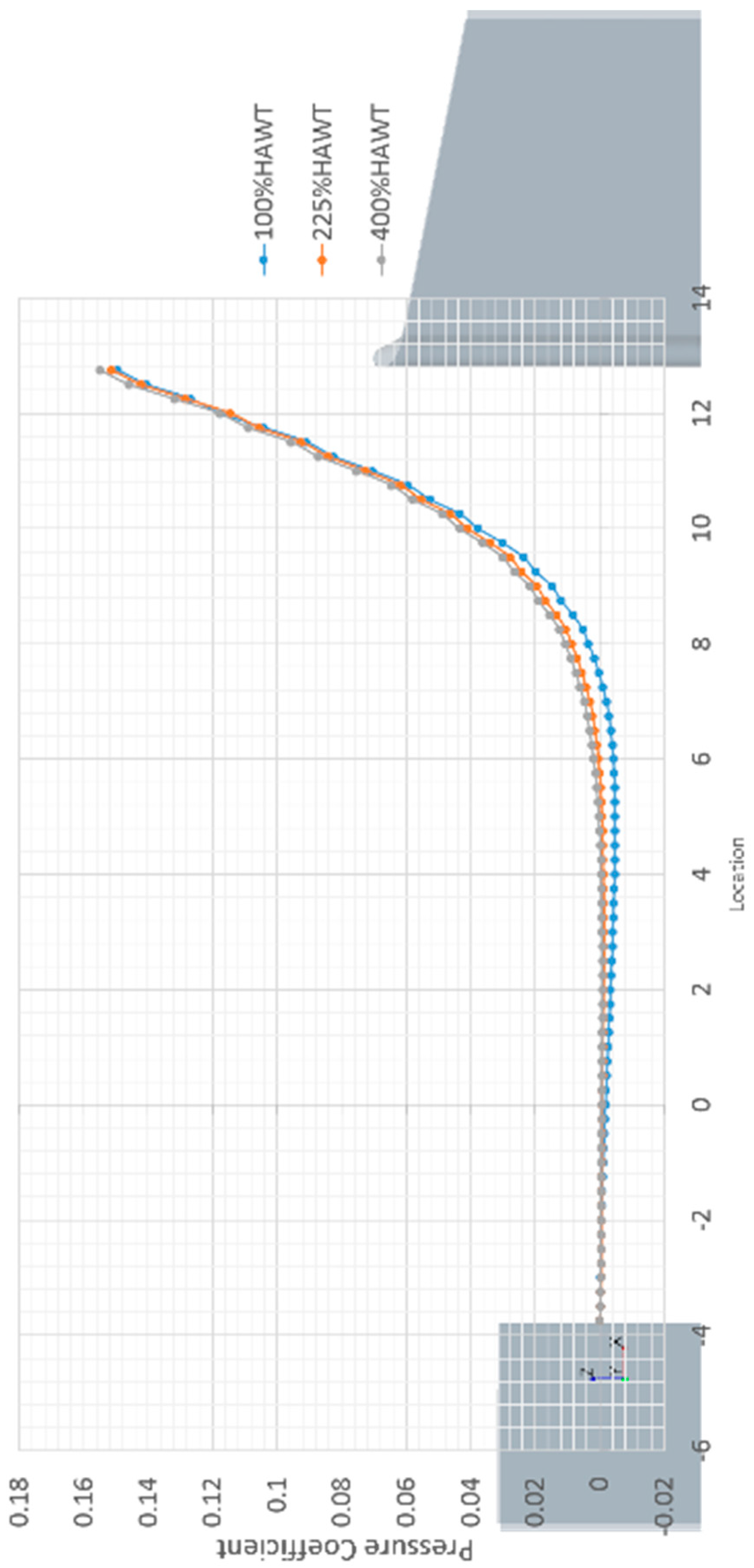
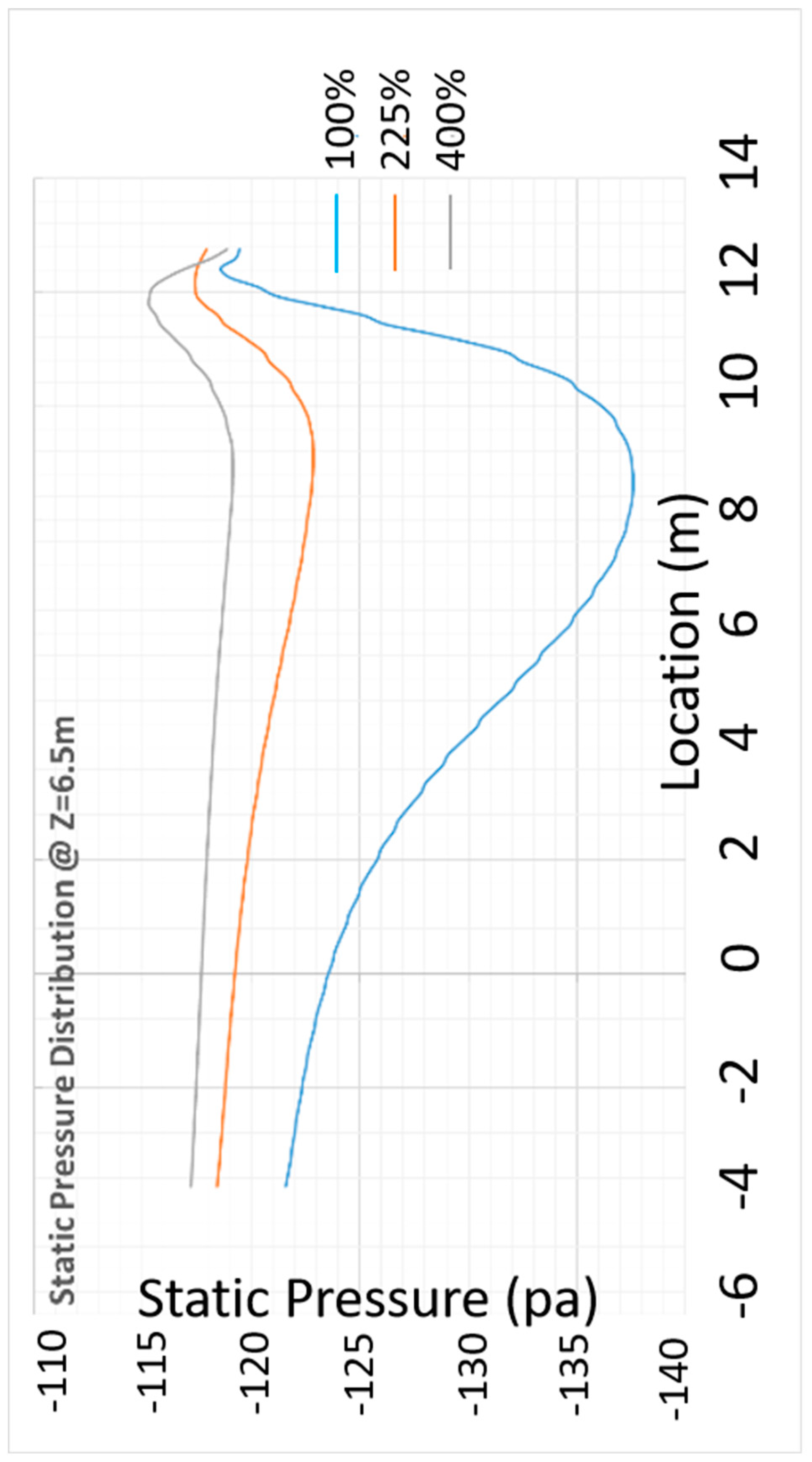
4.3. Blockage Effects of the Semi Open Jet Test Section

The frontal area of the virtual HAWT test section was expended by 225% and 400%, which resulted in reduced blockage ratios of 0.56% and 0.30%, respectively. The simulations were carried out with the moving ground and rotating wheel boundary conditions, and the results are presented in Table 5. All three scales ran without the vehicle model in the tunnel first, to obtain the pressure gradient in the empty plenum chamber. The mean static pressure coefficients along the center line of nozzle outlet are shown in Figure 14. It is noticeable, in the zoomed-in figure, that the original HAWT test section has a longitudinal negative pressure gradient in the empty model before it reaches the collector, resulting in an over-predicted drag value, since the negative pressure gradient causes the air flow to accelerate when passing over the test vehicle model. By keeping the nozzle and collector at the same location, but inflating the open jet test section in horizontal (Y) and vertical (Z) directions, the magnitude of that negative pressure gradient is reduced, becoming nearly zero when the test section was scaled up to 400% of its original size. The pressure gradient change caused a drag reduction for the larger test sections.
After putting the vehicle model into all three scales of the open jet test sections, (shown in Figure 15), the mean static pressure distributions on the center plane at different Z positions were measured. Figure 15 shows the five Z-locations of pressure probes. At all these locations, the original HAWT test section has the lowest static pressure, while the pressure in the plenum chamber increases with the increase of the test section volume. At Z = 3.5 m and above, the favorable pressure gradient in the 100% test section becomes obvious compared to other scales. At Z = 6.5 m, since it is close to the roof of the 100% domain, the favorable pressure gradient becomes stronger, while the pressure distributions in 225% and 400% scales also start turning favorable, as they are approaching to the top boundary.
The phenomenon of smaller test sections having lower static pressure in the plenum chamber of open jet wind tunnel, as Figure 16 indicates, can also be observed in Figure 17 and Figure 18, when the vehicle model is placed inside the tunnel, through the jet expansion change corresponding to different test section volumes. Both figures present the test section blockage effect on the semi-open jet expansion. From the side view of the center plane, the comparisons in Figure 17 show that the smaller plenum chamber causes the jet to expand earlier. The velocity magnitude in the outer layer of the jet is higher compared to the larger scale test-section models, which corresponds to higher dynamic pressure. As the total pressure of the domain remains constant, the static pressure in that region is relatively low.
As both the model and numerical representation of the HAWT domain are symmetric, additional features of this jet expansion can be observed using a XY-plane, covering only the right or left half of the simulation domain, which is presented in Figure 18. The velocity magnitude contour shows the original plenum chamber of HAWT forced the jet to expand much earlier than the other two larger-scale test-section models in the horizontal direction as well. The early expansion causes higher jet outer layer velocity at the nozzle outlet, as well as around the vehicle. With faster flow coming toward the test vehicle, the predicted drag coefficient of the model will be greater than that obtained from a larger test section with the same jet.
To summarize, the volume change of the open jet test section has a significant effect on the drag predictions of the test vehicle. The differences in drag coefficient measurements come from the streamwise pressure gradient change in the plenum chamber and the jet expansion rate. The smallest test section had a negative pressure gradient when tested as an empty tunnel, while a nearly zero pressure gradient was found in the larger scales. The early jet expansion causing faster jet flow passing the vehicle is another important contribution to the higher drag coefficient value in the 100% HAWT test section.

4.4. HAWT and Free-Air Tunnel Comparison

For a direct comparison between the aerodynamic characteristics observed in a limited area test section like the HAWT test section and those that might have been observed in the free air domain, Figure 19 compares the velocity magnitude contours on the center plane, when the vehicle model is placed in 100% HAWT model and in free air, respectively. For both cases, the flow field near the vehicle is similar except for the area above the roof (A), and the region above the hood-windshield conjunction (B). The deformation of the velocity contours in these regions for the HAWT simulations is because of the jet shear layer effect in the test section, which changes the flow velocity over the vehicle. As expected, the aerodynamic coefficients are overestimated in wind tunnel simulations compared to the free air domain.

5. Conclusions

In this paper, the full-scale model of 2014 Hyundai Veloster was tested in four different computational domains using a finite volume CFD code. The CFD simulations were validated with the wind tunnel test data from the Hyundai Aero-acoustic Wind Tunnel (HAWT) located at the Hyundai Namyang Technical Center in South Korea. The correlation results are encouraging. Although the CFD simulation over-predicted the drag coefficient by a small amount in the reproduced HAWT test section compared to the reported experimental data, the change in C D in CFD from the improved spoiler to the original spoiler closely matches the wind tunnel results.
The blockage effects of the open jet wind tunnel test section were evaluated by different scales of the plenum chamber, with a same longitudinal extent. A negative pressure gradient was found in the original empty HAWT test section in the streamwise direction, as well as an earlier jet expansion, which contributed to the higher drag predictions. By increasing the volume of the test section, the negative pressure gradient turned to a nearly zero pressure gradient before approaching the collector, and the jet expansion was delayed. As a result, the larger test sections have less interference effect on the test models in open jet wind tunnels, and the drag predictions are closer to the free air condition.
Two different ground plane boundary conditions, static floor with fixed wheels and moving ground with rotating wheels, were tested in both HAWT and free-air environments. The changes in vehicle drag and lift agree with the findings of Waschle [48]. These results also agree well with the works of Buscariolo et al. [24]. The reasons for the drag and lift reduction with moving floor and rotating wheels were explained by observing the change in tire wakes and underbody flow velocity from both top and side views; this study concluded that the reduction of the tire wake size is the primary attributer to drag reduction.

Author Contributions

Conceptualization, C.F., and M.U.; Investigation, C.F., M.U. and C.Z.; Methodology, C.F., M.U., and C.Z.; Supervision, M.U.; Validation, C.F., M.U. and C.Z.; Writing–original draft, C.F. and M.U.; Writing–review & editing, C.F., M.U., and C.Z. All authors have read and agreed to the published version of the manuscript.

Funding

This research received no external funding. However, Chen Fu and Chunhui Zhang were supported as Graduate Teaching Assistants by the UNC Charlotte Department of Mechanical Engineering and Engineer Science.

Acknowledgments

The authors thank UNC Charlotte College of Engineering MOSAIC Computing and University Research Computing for their consistent support.

Conflicts of Interest

The authors declare no conflict of interest.

References

  1. Kremheller, A. The Aerodynamics Development of the New Nissan Qashqai; 2014-01-0572; Society of Automotive Engineers: Detroit, MI, USA, 2014. [Google Scholar] [CrossRef]
  2. Katz, J. Race Car Aerodynamics: Designing for Speed; R. Bentley: Cambridge, MA, USA, 2006. [Google Scholar]
  3. Glauert, H. Wind Tunnel Interference on Wings, Bodies and Airscrews; DTIC Document, No. ARC-R/M-1566; Aeronautical Research Council: London, UK, 1933. [Google Scholar]
  4. Cooper, K. Closed-Test-Section Wind Tunnel Blockage Corrections for Road Vehicles; Special Publication SAE SP1176, Society of Automotive Engineers; SAE: Detroit, MI, USA, 1996. [Google Scholar]
  5. Mercker, E.; Wiedemann, J. On the Correction of Interference Effects in Open Jet Wind Tunnels; Technical Paper; SAE: Detroit, MI, USA, 1996. [Google Scholar]
  6. Mercker, E.; Wickern, G.; Wiedemann, J. Contemplation of Nozzle Blockage in Open Jet WindTunnels in View of Different ‘Q’ Determination Techniques; SAE 970136; Society of Automotive Engineers: Detroit, MI, USA, 1997. [Google Scholar]
  7. Wickern, G. On the Application of Classical Wind Tunnel Corrections for Automotive Bodies; 2001-01-0633; Society of Automotive Engineers: Detroit, MI, USA, 2001. [Google Scholar] [CrossRef]
  8. Wickern, G.; Schwartekopp, B. Correction of Nozzle Gradient Effects in Open Jet Wind Tunnels; 2004-01-0669; Society of Automotive Engineers: Detroit, MI, USA, 2004. [Google Scholar] [CrossRef]
  9. Hoffman, J.; Martindale, B.; Arnette, S.; Williams, J.; Wallis, S. Effect of Test Section Configuration on Aerodynamic Drag Measurements; 2001-01-0631; Society of Automotive Engineers: Detroit, MI, USA, 2001. [Google Scholar] [CrossRef]
  10. Hoffman, J.; Martindale, B.; Arnette, S.; Williams, J.; Wallis, S. Development of Lift and Drag Corrections for Open Jet Wind Tunnel Tests for an Extended Range of Vehicle Shapes; 2003-01-0934; Society of Automotive Engineers: Detroit, MI, USA, 2003. [Google Scholar] [CrossRef]
  11. Mercker, E.; Cooper, K.R.; Fischer, O.; Wiedemann, J. The Influence of a Horizontal Pressure Distribution on Aerodynamic Drag in Open and Closed Wind Tunnels; 2005-01-0867; Society of Automotive Engineers: Detroit, MI, USA, 2005. [Google Scholar] [CrossRef]
  12. Mercker, E.; Cooper, K.R. A Two-Measurement Correction for the Effects of a Pressure Gradient on Automotive, Open-Jet, Wind Tunnel Measurements; 2006-01-0568; Society of Automotive Engineers: Detroit, MI, USA, 2006. [Google Scholar] [CrossRef]
  13. Lounsberry, T.; Walter, J. Practical Implementation of the Two-Measurement Correction Method in Automotive Wind Tunnels. SAE Int. J. Passeng. Cars Mech. Syst. 2015, 8, 676–686. [Google Scholar] [CrossRef]
  14. Gleason, M. CFD Analysis of Various Automotive Bodies in Linear Static Pressure Gradients; 2012-01-0298; Society of Automotive Engineers: Detroit, MI, USA, 2012. [Google Scholar] [CrossRef]
  15. Gleason, M.E.; Lounsberry, T.; Sbeih, K.; Surapaneni, S. CFD Analysis of Automotive Bodies in Static Pressure Gradients; 2014-01-0612; Society of Automotive Engineers: Detroit, MI, USA, 2014. [Google Scholar] [CrossRef]
  16. Hucho, W.-h.; Sovran, G. Aerodynamics of road vehicles. Ann. Rev. Fluid Mech. 1993, 25, 485–537. [Google Scholar] [CrossRef]
  17. Soares, R.F.; Garry, K.F.; Holt, J. Comparison of the Far-Field Aerodynamic Wake Development for Three Drivaer Model Configurations using a Cost-Effective RANS Simulation; 2017-01-1514; Society of Automotive Engineers: Detroit, MI, USA, 2017. [Google Scholar]
  18. Aljure, D.E.; Calafell, J.; Baez, A.; Oliva, A. Flow over a realistic car model: Wall modeled large eddy simulations assessment and unsteady effects. J. Wind Eng. Ind. Aerodyn. 2018, 174, 225–240. [Google Scholar] [CrossRef] [Green Version]
  19. Roy, A.; Dasgupta, D. Towards a novel strategy for safety, stability and driving dynamics enhancement during cornering manoeuvres in motorsports applications. Sci. Rep. 2020, 10, 1–14. [Google Scholar] [CrossRef] [PubMed] [Green Version]
  20. Gaylard, A.P. The Appropriate Use of CFD in the Automotive Design Process; 2009-01-1162; Society of Automotive Engineers: Detroit, MI, USA, 2009. [Google Scholar] [CrossRef]
  21. Ueno, D.; Hu, G.; Komada, I.; Otaki, K.; Fan, Q. CFD Analysis in Research and Development of Racing Car; 2006-01-3646; Society of Automotive Engineers: Detroit, MI, USA, 2006. [Google Scholar] [CrossRef]
  22. Cyr, S.; Ih, K.D.; Park, S.H. Accurate Reproduction of Wind-Tunnel Results with CFD; 2011-01-0158; Society of Automotive Engineers: Detroit, MI, USA, 2011. [Google Scholar] [CrossRef]
  23. Wickern, G.; Dietz, S.; Luehrmann, L. Gradient Effects on Drag Due to Boundary-Layer Suction in Automotive Wind Tunnels; 2003-01-0655; Society of Automotive Engineers: Detroit, MI, USA, 2003. [Google Scholar] [CrossRef]
  24. Buscariolo, F.F.; de Campos Mariani, A.L. Analysis of Different Types of Wind Tunnel’s Ground Configuration Using Numerical Simulation; 2010-36-0078; Society of Automotive Engineers: Detroit, MI, USA, 2010. [Google Scholar] [CrossRef]
  25. Hennig, A.; Widdecke, N.; Kuthada, T.; Wiedemann, J. Numerical Comparison of Rolling Road Systems. SAE Int. J. Engines 2011, 4, 2659–2670. [Google Scholar] [CrossRef]
  26. Meederira, P.; Fadler, G.; Uddin, M. Numerical Investigation on the Characterization of Interaction Between the Tire-Wake-Vortices and 5-Belt MGP Turntable; SAE Technical Paper 2020-01-0683; Society of Automotive Engineers: Detroit, MI, USA, 2020. [CrossRef]
  27. Koitrand, S.; Lofdahl, L.; Rehnberg, S.; Gaylard, A. A Computational Investigation of Ground Simulation for a Saloon Car. SAE Int. J. Commer. Veh. 2014, 7, 111–123. [Google Scholar] [CrossRef]
  28. Wäschle, A.; Cyr, S.; Kuthada, T.; Wiedemann, J. Flow Around an Isolated Wheel—Experimental and Numerical Comparison of Two CFD Codes; 2004-01-0445; Society of Automotive Engineers: Detroit, MI, USA, 2004. [Google Scholar] [CrossRef]
  29. Elofsson, P.; Bannister, M. Drag Reduction Mechanisms Due to Moving Ground and Wheel Rotation in Passenger Cars; 2002-01-0531; Society of Automotive Engineers: Detroit, MI, USA, 2002. [Google Scholar] [CrossRef]
  30. Misar, A.S.; Uddin, M.; Robinson, A.; Fu, C. Numerical Analysis of Flow around an Isolated Rotating Wheel Using a Sliding Mesh Technique; 2020-01-0675 SAE Technical Paper; Society of Automotive Engineers: Detroit, MI, USA, 2020. [Google Scholar]
  31. Fischer, O.; Kuthada, T.; Mercker, E.; Wiedemann, J.; Duncan, B. CFD Approach to Evaluate Wind-Tunnel and Model Setup Effects on Aerodynamic Drag and Lift for Detailed Vehicles; 2010-01-0760; Society of Automotive Engineers: Detroit, MI, USA, 2010. [Google Scholar] [CrossRef]
  32. Kandasamy, S.; Duncan, B.; Gau, H.; Maroy, F.; Belanger, A.; Gruen, N.; Schäufele, S. Aerodynamic Performance Assessment of BMW Validation Models using Computational Fluid Dynamics; 2012-01-0297; Society of Automotive Engineers: Detroit, MI, USA, 2012. [Google Scholar] [CrossRef]
  33. Ashton, N.; West, A.; Lardeau, S.; Revell, A. Assessment of RANS and DES methods for realistic automotive models. Comput. Fluids 2016, 128, 1–15. [Google Scholar] [CrossRef] [Green Version]
  34. Guilmineau, E.; Deng, G.B.; Leroyer, A.; Queutey, P. Assessment of hybrid RANS-LES formulations for flow simulation around the Ahmed body. Comput. Fluids 2018, 176, 302–319. [Google Scholar] [CrossRef]
  35. Zhang, C.; Bounds, C.P.; Foster, L.; Uddin, M. Turbulence Modeling Effects on the CFD Predictions of Flow over a Detailed Full-Scale Sedan Vehicle. Fluids 2019, 4, 148. [Google Scholar] [CrossRef] [Green Version]
  36. Fu, C.; Uddin, M.; Robinson, C.; Guzman, A.; Bailey, D. Turbulence models and model closure coefficients sensitivity of NASCAR Racecar RANS CFD aerodynamic predictions. SAE Int. J. Passeng. Cars-Mech. Syst. 2017, 10, 330–344. [Google Scholar] [CrossRef]
  37. Fu, C.; Uddin, M.; Robinson, A.C. Turbulence modeling effects on the CFD predictions of flow over a NASCAR Gen 6 racecar. J. Wind Eng. Ind. Aerodyn. 2018, 176, 98–111. [Google Scholar] [CrossRef]
  38. Fu, C.; Uddin, M.; Selent, C. The Effect of Inlet Turbulence Specifications on the RANS CFD Predictions of a NASCAR Gen-6 Racecar; No. 2018-01-0736 SAE Technical Paper; Society of Automotive Engineers: Detroit, MI, USA, 2018. [Google Scholar]
  39. Fu, C.; Bounds, C.; Uddin, M.; Selent, C. Fine Tuning the SST k− ω Turbulence Model Closure Coefficients for Improved NASCAR Cup Racecar Aerodynamic Predictions. SAE Int. J. Adv. Curr. Pract. Mobil. 2019, 1, 1226–1232. [Google Scholar] [CrossRef]
  40. Fu, C.; Bounds, C.P.; Selent, C.; Uddin, M. Turbulence modeling effects on the aerodynamic characterizations of a NASCAR Generation 6 racecar subject to yaw and pitch changes, Proceedings of the Institution of Mechanical Engineers. Part D J. Autom. Eng. 2019, 233, 3600–3620. [Google Scholar] [CrossRef]
  41. Connor, C.; Kharazi, A.; Walter, J.; Martindale, B. Comparison of Wind Tunnel Configurations for Testing Closed-Wheel Race Cars: A CFD Study; 2006-01-3620; Society of Automotive Engineers: Detroit, MI, USA, 2006. [Google Scholar] [CrossRef]
  42. Kim, M.S.; Lee, J.H.; Kee, J.D.; Chang, J.H. Hyundai Full Scale Aero-acoustic Wind Tunnel; 2001-01-0629; Society of Automotive Engineers: Detroit, MI, USA, 2001. [Google Scholar] [CrossRef]
  43. Fischer, O.; Kuthada, T.; Wiedemann, J.; Dethioux, P.; Mann, R.; Duncan, B. CFD Validation Study for a Sedan Scale Model in an Open Jet Wind Tunnel; 2008-01-0325; Society of Automotive Engineers: Detroit, MI, USA, 2008. [Google Scholar] [CrossRef]
  44. Shih, T.H.; Liou, W.W.; Shabbir, A.; Yang, Z.; Zhu, J. A New k-Epsilon Eddy Viscosity Model for High Reynolds Number Turbulent Flows: Model Development and Validation; NASA-TM-106721; NASA Lewis Research Center: Cleveland, OH, USA, 1994. [Google Scholar]
  45. Menter, F.R. Improved two-equation k-omega turbulence models for aerodynamic flows. NASA STI/Recon Tech. Rep. News 1992, 93, 22809. [Google Scholar]
  46. Cooper, K.R.; Mercker, E.; Müller, J. The necessity for boundary corrections in a standard practice for the open-jet wind tunnel testing of automobiles. Proceedings of the Institution of Mechanical Engineers. Part D J. Autom. Eng. 2017, 231, 1245–1273. [Google Scholar] [CrossRef]
  47. Glauert, H. Wind Tunnel Interference on Wings, Bodies and Airscrews. Aeronautical Research Committee Reports and Memoranda 1566; HM Stationery Office: London, UK, 1933. [Google Scholar]
  48. Wäschle, A. The Influence of Rotating Wheels on Vehicle Aerodynamics—Numerical and Experimental Investigations; 2007-01-0107; Society of Automotive Engineers: Detroit, MI, USA, 2007. [Google Scholar] [CrossRef]
Figure 1. Computational fluid dynamics (CFD) representation of the Hyundai Aero-Acoustic Wind Tunnel (HAWT) test section, drawn using the geometry details given in Kim et al. [42].
Vehicles 02 00018 g001
Figure 2. Top and side views of the computational domain used for various blockage ratios, based on the HAWT baseline tunnel, as used by Kim et al. [42].
Vehicles 02 00018 g002
Figure 3. Schematics of the blockage-free tunnel.
Vehicles 02 00018 g003
Figure 4. Top views of the original (a) and improved (b) spoilers.
Vehicles 02 00018 g004
Figure 5. Side views of the original (a) and improved (b) spoiler.
Vehicles 02 00018 g005
Figure 6. Mesh on the center plane of the model.
Vehicles 02 00018 g006
Figure 7. Blockage-free domain mesh.
Vehicles 02 00018 g007
Figure 8. Top (top figure) and side (bottom figure) views of the spoiler mesh.
Vehicles 02 00018 g008
Figure 9. Cross-sections layout.
Vehicles 02 00018 g009
Figure 10. Streamwise mean velocity on a Z-plane at Z = 0.05 (plane 4) for static floor vs. moving ground with vehicle placed inside HAWT.
Vehicles 02 00018 g010
Figure 11. Velocity magnitude for the static floor and moving belt cases with the vehicle in HAWT model; the Y-plane is taken through the right-tire center at Y = 0.78 (plane 2).
Vehicles 02 00018 g011
Figure 12. Streamwise mean velocity on a Z-plane at Z = 0.05 (plane 4) for static floor vs. moving ground with vehicle placed in blockage free environment.
Vehicles 02 00018 g012
Figure 13. Velocity magnitude for the static floor and moving belt cases with the vehicle in free air environment; the Y-plane is taken through the right-tire center at Y = 0.78 (plane 2).
Vehicles 02 00018 g013
Figure 14. Empty test section static pressure coefficients in the longitudinal direction along the nozzle centerline.
Vehicles 02 00018 g014
Figure 15. Static pressure probes layout.
Vehicles 02 00018 g015
Figure 16. Static pressure distributions on center plane at different Z locations; from top to bottom Z = 2.5 m, 3.5 m, 4.5 m, 5.5 m, and 6.5 m, respectively. Please see Figure 15 for the reference of these Z -locations with respect to vehicle.
Vehicles 02 00018 g016aVehicles 02 00018 g016bVehicles 02 00018 g016c
Figure 17. Mean velocity magnitude on a Y-plane along the vehicle centerline.
Vehicles 02 00018 g017
Figure 18. Mean velocity magnitude at nozzle outlet (top view).
Vehicles 02 00018 g018
Figure 19. Velocity magnitude for free air and 100% HAWT model a Y-plane along the vehicle centerline.
Vehicles 02 00018 g019
Table 1. Computational grid levels vs. grid sizes.
Grid Level12345
Grid Size (mm)244896192384
Table 2. Tabulated values of drag coefficient C D .
C D Original SpoilerImproved Spoiler C D
Wind-tunnel0.3280.3260.002
CFD0.3380.3360.002
Table 3. Drag coefficient values obtained from the static and moving ground plane CFD simulations with the vehicle model placed inside the HAWT.
HAWT   ( C D ) Original SpoilerImproved Spoiler
Static Floor0.3380.336
Moving Floor0.3330.331
C D 0.0050.005
Table 4. Influence of moving ground and rotating wheels on drag and lift coefficients.
HAWT C D C L
Static Floor0.3380.157
Moving Floor0.3330.105
Delta ( )0.0050.052
Free Air C D C L
Static Floor0.3260.140
Moving Floor0.3200.098
Delta ( )0.0060.042
Table 5. Effect of blockage ratio on drag prediction.
Test Section Blockage Ratio1.25% (HAWT)0.56%0.30%0.04%
C D 0.3330.3280.3250.320

