Vacuum Interaction of Topological Strings at Short Distances

Abstract

The paper provides an extended overview of recent results obtained by the authors in the process of studying the vacuum interaction of topological cosmic strings at short distances, taking into account their transverse size a and the mass m of the quantized field. We consider the case of a massive real-valued scalar field with minimal coupling. It is shown that at the interstring distances significantly larger than the Compton length, $l_c=1/m$, the Casimir effect is damped exponentially. On the other hand, at distances smaller than $l_c$ but much larger than the typical string width, the field-mass influence becomes insignificant. In this case, the partial contribution of a massive field to the Casimir energy is of the same order as the contribution of a massless one. At these distances, the string’s transverse size is insignificant also. However, at the interstring distances of the same order as a string radius, the energy of the vacuum interaction of thick strings may significantly surpass the one for two infinitely thin strings with the same mass per unit length.

1. Introduction

Seventy-five years ago, a phenomenon was predicted [1] and then named the Casimir effect in honor of the author. Being experimentally confirmed, it became direct evidence of the close relationship between the macroscopic external conditions and quantized fields. Since those times, it has shown great development, both in experimental investigations and at the level of theoretical research. Now, it is a subject of study not only by specialists in quantum field theory and physics of condensed matter and nanotechnology but also by scientists working in various fields of gravity and cosmology (see, e.g., [2]).

One of the problems related to modern astrophysics, which was considered in the literature, is the problem of the vacuum interaction of cosmic strings.

Cosmic strings are considered as one-dimensional-extended topological defects (closed or infinite), which might be created under cosmological phase transitions during the Universe evolution [3,4]. In what follows, we use the term “string” for this kind of cosmic string (so-called topological cosmic strings) and do not consider the case of non-topological F-strings and D-strings, which may be formed during the interaction of multidimensional branes.

A special interest in these types of defects arose in connection with the hypothesis that they might represent one of the basic sources of primary fluctuations in the Hot Universe. The hypothesis was not confirmed, but the cosmic strings are still considered to be a possible origin of some observable effects (a review of the possible appearance and indirect effects of cosmic strings is to be found in Ref. [5]). This stimulates the searches for ways to detect cosmic strings and, consequently, the investigation of features concerning how classical (or quantum) matter behaves in the corresponding curved backgrounds.

The study of the evolution of the cosmic-string net during its formation in the Early Universe phase transitions implies that the investigations of processes happened under close contact of strings and collisions [3,4]. In these processes, the account of the vacuum (Casimir) string interaction may turn out to be significant.

The first estimate of the energy of Casimir of two parallel infinitely thin strings was obtained in Ref. [6]. Subsequently, the result of this study was corrected in Refs. [7,8,9].

In papers [7,9], the authors proceeded within the framework of a local formalism, where the object of study was the renormalized vacuum average of the energy–momentum tensor (EMT) operator. In paper [8], a global formalism was applied, which allowed us to work directly with the renormalized total vacuum energy. In studies [7,8,9], the direct product of the two-dimensional Minkowski space and a two-dimensional locally flat surface with two conical singularities was chosen as the spacetime model.

Meanwhile, the creation and evolution of cosmic strings do not imply that they are necessarily parallel. In Ref. [10], the global formalism was extended to the different mutual directions of strings. The Casimir energy due to the massless scalar field and infinitely thin strings was computed for two interacting straight strings.

However, the string’s radius is determined by the energy scale of that phase transition with broken symmetry when the string was created, and for the GUT strings, the radius has an estimate of $a\sim {10}^{-28}\mathrm{cm}$. At these scales, the cone vertex represents not just a point-like singularity but also the curvature, distributed over a cylindrical region of radius a, while the metric should smoothly transit to the external conical domain. Therefore, it raises the following question: how does the transverse string size influence the quantum field effects near the strings?

In the meantime, another problem concerns the influence of the quantized field’s mass on the Casimir effect. It is natural to suppose that the characteristic lengthy scale, where the mass is significant, is a Compton length. Quantitatively, the latter is much larger (for all known elementary particles) than the transverse size of Grand Unified Theory (GUT) strings.

The effects of the finite core on the vacuum polarization around a single cosmic string have been investigated earlier, and some nontrivial field-theory effects have been discovered [11,12,13,14,15,16,17]. In the present paper, we perform the next step and consider the Casimir effect arising in the net of parallel cosmic strings, taking into account not only the non-zero strings’ widths but also the non-zero field’s mass.

The striking feature of the multi-string background is that, due to translational symmetry along the z-axis, it is enough to analyze the geometry in the two-dimensional plane transverse to the string net. Inside this plane, the scalar curvature does not vanish only on a system of non-overlapping compact domains. As a result, the direct gravitational interstring interaction is absent. However, the global distinction of the spacetime considered here, from the Minkowski one, leads to a change in the spectrum of vacuum fluctuations and, consequently, to the appearance of the interstring attraction force, the Casimir effect.

Let us start with a qualitative analysis of the problem. First, to notice is that the energy (per unit string’s length) of vacuum interaction has a dimensionality of the inverse length square. Thus, from the dimensional quantities in the problem considred here, it can depend only upon the interstring distance, d, the string radius, a, and the field’s Compton length, $l_c=1/m$.

Then the relative energy (per unit length) of the interaction of two similar strings, parallel to the z-axis, in the units of G = ħ = c = 1 (where G denotes the Newtonian constant of gravity, ħ the Planck’s constant, and c the speed of light) can be presented in the form

$$\begin{array}{c}\hfill \frac{{\mathcal{E}}_{\mathrm{Cas}}}{Z}=-\frac{4}{15\pi }\frac{{\mu }_1{\mu }_2}{d^2}\mathcal{F}\left(\frac{a}{d},md\right),Z=\int dz,\end{array}$$

(1)

where ${\mu }_{1,2}$ is the strings’ masses per unit length, while $\mathcal{F}$ is a real-valued function. The pre-factor just in front of $\mathcal{F}$ is determined using dimensional analysis and is specified to be equal to the Casimir energy of two infinitely thin strings interacting via the massless scalar field with minimal coupling. Let us note that with that choice of the pre-factor, the function $\mathcal{F}$ tends to unit as $a/d\to 0^{+}$ or $md\to 0^{+}$. Actually, the vanishing of these arguments can be interpreted both as neglect of the strings’ radii and as a transition to the massless field.

Hereafter, we restrict the study to the case of the scalar field with minimal coupling. It is related to the observation that for the case of the infinitely thin string, the non-zero coupling leads to the appearance of a potential with the Aharonov-Bohm $\delta$-like singularities in the field equation. Such an appearance takes special attention, and the computational results may drastically vary, in dependence on how one interprets these singularities [18,19].

However, the Compton length of the most massive currently known particle (the t-quark) is $l_c\sim {10}^{-15}\mathrm{cm}$, while the width of GUT strings is estimated as $a\sim {10}^{-28}\mathrm{cm}$, what is of many orders less. If one considers the distances $d\gg a$ then strings are to be approximately considered to be infinitely thin, and hence, in Equation (1), one can replace

$$\mathcal{F}\left(\frac{a}{d},md\right)\to {\mathcal{F}}_1\left(md\right)=\mathcal{F}\left(0,md\right).$$

Now let us estimate the behavior of ${\mathcal{F}}_1\left(md\right)$ as $md$ tends to zero. This limit can be regarded as a transition to the massless field limit with finite values d, and consequently, with the choice of a pre-factor in Equation (1), one has ${\mathcal{F}}_1=1$ in this limit. On the other hand, equally, this limit can be regarded as a transition $d\to 0^{+}$ (for infinitely thin strings), keeping the mass fixed. Therefore, the scale where the mass influence is significant is a Compton length. Thus, at interstring distances of the order of $l_c$ or smaller, the influence of mass is significant, and the partial contribution of massive modes into the vacuum energy is comparable with the one of a massless field. But for finite strings’ width, if one considers the distances $2a<d\ll l_c$, then the string transverse size cannot be neglected. However, if the above estimates hold, in this regime, one can neglect the field’s mass and carry out another substitution in Equation (1):

$$\mathcal{F}\left(\frac{a}{d},md\right)\to {\mathcal{F}}_2\left(\frac{a}{d}\right)=\mathcal{F}\left(\frac{a}{d},0\right).$$

In what follows, the length scale, where the transverse strings’ size is significant, is the string radius. Thus again, as soon as $\tilde{z}=a/d\to 0^{+}$ the function ${\mathcal{F}}_2$ tends to unity. Actually, if this limit is to be regarded as limit $d\to \infty$, then it is quite evident that at these distances, strings interact as infinitely thin ones. Consequently, the result should reproduce the Casimir energy of interaction of two infinitely thin strings, with the coefficient ${\mathcal{F}}_2=1$. The same limit is to be valid if a tends to zero. But for the finite-width (or, equivalently, ”thick”) strings, one has $d⩾2a$. Hence, the significant difference ${\mathcal{F}}_2$ from unity (and the significant difference of the Casimir energy from the strings’ width) should take place if the interstring distance does not significantly exceed $2a$.

Below, it is explicitly shown that these qualitative estimates are fully confirmed.

Actually, there is a variety of string models. Some of them imply that the gravity-induced Casimir force is not the only interaction. We compute a partial contribution to the total interstring interaction within any model, for which the above assumptions on the metric hold.

The computation is carried out within the so-called tr-ln formalism for the effective action, where one starts from the expression for the total vacuum energy, expressed in terms of the effective action.

Throughout the paper, we use the system of units G = ħ = c = 1; the metric signature is $(+,-,-,-)$.

2. Multi-String Spacetime

Consider the following four-dimensional spacetime, which represents the Cartesian product of two-dimensional Minkowski space and two-dimensional Riemannian manifold. The observation that any two-dimensional Riemannian surface is locally conformal to the Euclidean plane allows the reduction, by the appropriate coordinate transformation, of the four-dimensional metric to the form

$$\begin{array}{c}\hfill d{s}^2=d{t}^2-d{z}^2-{\mathrm{e}}^{-\sigma \left(\mathit{x}\right)}\left(d{x}_1^2+d{x}_2^2\right),\end{array}$$

(2)

where $x_1$ and $x_2$ are the two-dimensional Riemannian space coordinates and t denotes the time.

Let

$$\begin{array}{c}\hfill \sigma \left(\mathit{x}\right)=\sum _{\alpha }{\sigma }_{\alpha }\left(|\mathit{x}-{\mathit{x}}_{\alpha }|\right),|\mathit{x}-{\mathit{x}}_{\alpha }|={\left[{(x_1-x_{\alpha 1})}^2+{(x_2-x_{\alpha 2})}^2\right]}^{1/2}.\end{array}$$

(3)

Then the Ricci scalar reads:

$$\begin{array}{c}\hfill R=\sum _{\alpha }{R}_{\alpha }=\sum _{\alpha }{\mathrm{e}}^{\sigma }\Delta {\sigma }_{\alpha },\end{array}$$

(4)

where $\Delta$ stands for the Laplacian associated with two-dimensional Euclidean metric in the transverse subspace. If the supports of partial contributions, $\Delta {\sigma }_{\alpha }$, are compact and do not intersect each other, one deals with ultra-static spacetime, where the curvature is non-zero in a series of non-overlapping domains.

Choose the functions ${\sigma }_{\alpha }$ in the form

$${\sigma }_{\alpha }\left(\mathit{x}\right)=2(1-{\beta }_{\alpha })f_{\alpha }\left(r_{\alpha }\right)\theta \left(a_{\alpha }-r_{\alpha }\right)+2(1-{\beta }_{\alpha })ln\frac{r_{\alpha }}{a_{\alpha }}\theta \left(r_{\alpha }-a_{\alpha }\right),$$

(5)

where $a_{\alpha }$ is a conformal radius of $\alpha$th string, all parameters ${\beta }_{\alpha }⩽1$, $\theta (·)$ stands for the Heaviside step-function, and f is a twice-differentiable function of an argument $r_{\alpha }=|\mathit{x}-{\mathit{x}}_{\alpha }|$, which satisfies the following boundary conditions:

$$\begin{array}{c}\hfill f_{\alpha }{|}_{r_{\alpha }=a_{\alpha }}=0,\frac{d{f}_{\alpha }}{d{r}_{\alpha }}{|}_{r_{\alpha }=a_{\alpha }}=\frac{1}{a_{\alpha }}.\end{array}$$

(6)

With such a choice of the conformal factor, ${\mathrm{e}}^{-\sigma }$, the scalar curvature vanishes everywhere if $|\mathit{x}-{\mathit{x}}_{\alpha }|>a_{\alpha }$ holds for all $\alpha$. Moreover, in this domain, the metric coincides with that of a system of parallel infinitely thin cosmic strings [20]. Furthermore, the criterion of the perturbation smallness and thus the validity of calculations within the perturbation theory is a smallness of parameters $(1-{\beta }_{\alpha })$. It is assumed that for the GUT strings, the estimate of these parameters is ${10}^{-6}$.

Therefore, the space defined above is to be regarded as a spacetime generated by the net of parallel cosmic strings with non-zero width. The scalar curvature of this spacetime reads:

$$R\left(\mathit{x}\right)=\left\{\begin{array}{ccc}{\mathrm{e}}^{\sigma }\Delta {\sigma }_{\alpha },\hfill & \mathrm{if}\mathrm{exists}\alpha :\hfill & |\mathit{x}-{\mathit{x}}_{\alpha }| ⩽ a_{\alpha };\hfill \\ 0,\hfill & \mathrm{if}\mathrm{for}\mathrm{all}\alpha \hfill & |\mathit{x}-{\mathit{x}}_{\alpha }| > a_{\alpha }.\hfill \end{array}\right.$$

(7)

The metric under consideration satisfies the Einstein equation, where on the right-hand side, the energy-momentum tensor has the following time component:

$$T_{tt}=\frac{R}{16\pi }=\frac{1}{16\pi }{\mathrm{e}}^{\sigma }\sum _{\alpha }\Delta {\sigma }_{\alpha }.$$

Hence, the energy per unit length of a system of thick strings equals

$$\int T_{tt}\sqrt{-g}{d}^{2}x=\frac{1}{16\pi }\sum _{\alpha }\int d^{2}x\Delta {\sigma }_{\alpha }=\frac{1-{\beta }_{\alpha }}{8\pi }\sum _{\alpha }\int d^{2}x\Delta f_{\alpha },$$

where g is the determinant of the metric tensor.

In what follows, the quantity

$$\begin{array}{c}\hfill {\mu }_{\alpha }:=\frac{1-{\beta }_{\alpha }}{8\pi }\int d^{2}x\Delta f_{\alpha }\end{array}$$

(8)

is to be regarded as the energy per unit length of the $\alpha$th string.

The transition to the infinitely thin strings implies the limit of any support $\Delta {\sigma }_{\alpha }$ to be the single dot $\mathit{x}={\mathit{x}}_{\alpha }$, preserving the value of integrals over $d^{2}x$. This limit (as $a_{\alpha }\to 0^{+}$) corresponds to the fixation of the linear energy density of any string. In this limit, the exponential power in Equation (2) goes to

$$\begin{array}{c}\hfill \sigma \left(\mathit{x}\right)=2\sum _{\alpha }(1-{\beta }_{\alpha })ln|\mathit{x}-{\mathit{x}}_{\alpha }|.\end{array}$$

(9)

Then, regarding the limit in the distributional sense, one obtains:

$$\begin{array}{c}\hfill \underset{a_{\alpha }\to 0^{+}}{lim}\Delta {\sigma }_{\alpha }=4\pi (1-{\beta }_{\alpha }){\delta }^2(\mathit{x}-{\mathit{x}}_{\alpha }).\end{array}$$

(10)

Therefore, in addition to Equation (6), when specifying the functions $f_{\alpha }$, one has to demand

$$\int d^{2}x\Delta f_{\alpha }=2\pi .$$

Then from Equation (8), one obtains

$${\mu }_{\alpha }=\frac{1-{\beta }_{\alpha }}{4},$$

and, in the limit $a_{\alpha }\to 0^{+}$, the heuristic expression,

$$\begin{array}{c}\hfill T_{tt}\left(\mathit{x}\right)={\mathrm{e}}^{\sigma \left(\mathit{x}\right)}\sum _{\alpha }{\mu }_{\alpha }{\delta }^2(\mathit{x}-{\mathit{x}}_{\alpha }),\end{array}$$

(11)

holds.

As shown in Ref. [20], any two-dimensional $x_1{x}_2$-plane represents the locally flat surface with a series of conical singularities located at the points ${\mathit{x}}_{\alpha }$, while the parameter $(1-{\beta }_{\alpha })$ represents the angular deficit, related to $\alpha$th conical vertex

$$\delta {\phi }_{\alpha }=8\pi {\mu }_{\alpha }=2\pi (1-{\beta }_{\alpha }).$$

Hereafter, we assume that the conformal coordinates cover the $x_1{x}_2$-plane globally. In the case of single singularity, it takes place if $\mu <1/4$, while in the case of more singularities—if the restriction $\sum {\mu }_{\alpha }<1/2$ holds and thus the conical subspace does not acquire the sphere topology [21,22,23,24].

In the case of a single infinitely thin string, the spacetime metric has two striking features: (i) the absence of any length parameters and (ii) higher symmetry. The first allows us to state that for a massless field, the vacuum expectation value of the EMT depends upon the distance, r, from the observation point to the singularity. In four dimensions of a spacetime the EMT scales as

$${\langle T_{\mu \nu }\rangle }_{\mathrm{vac}}\sim r^{-4}$$

with $\mu$, $\nu$ the four-dimensional indices.

The second feature allows the separation of variables in the field equation to construct Green’s function analytically and to compute the renormalized ${\langle T_{\mu \nu }\rangle }_{\mathrm{vac}}$. In the case of two strings and more, the problem becomes too complicated, and the perturbation theory techniques become of particular significance [7,8,9].

The transition to the finite-width strings complicates the problem and demands the concretization of functions ${\sigma }_{\alpha }$. The smoothing of the cone vertices can be realized with the following choice of the functions $f_{\alpha }$ [25,26]:

$$\begin{array}{c}\hfill f_{\alpha }\left(r_{\alpha }\right)=-\frac{1}{2}\left(1-\frac{r_{\alpha }^2}{a_{\alpha }^2}\right).\end{array}$$

(12)

Now, the Ricci scalar is given by

$$R\left(\mathit{x}\right)=\left\{\begin{array}{ccc}4(1-{\beta }_{\alpha }){\mathrm{e}}^{\sigma }/a_{\alpha }^2,\hfill & \mathrm{if}\mathrm{exists}\alpha :\hfill & |\mathit{x}-{\mathit{x}}_{\alpha }| ⩽ a_{\alpha };\hfill \\ 0,\hfill & \mathrm{if}\mathrm{for}\mathrm{all}\alpha \hfill & |\mathit{x}-{\mathit{x}}_{\alpha }| > a_{\alpha }.\hfill \end{array}\right.$$

This model is known as the ”ballpoint-pen” model, and below, when considering the Casimir effect in a system of thick strings, we restrict ourselves to this particular case.

For a single cosmic string, the schematic illustrations of a two-dimensional section for the infinitely thin string and the ”smoothed” one are shown in Figure 1.

3. The Setup

The action of the real-valued scalar field $\varphi$ with mass m can be chosen in the form

$$S_{\varphi }=-\frac{1}{2}\int d^{4}x\varphi \left(x\right)L(x,\partial )\varphi \left(x\right),$$

where the field operator $L(x,\partial )=\sqrt{-g}(\square +m^2)$ and $\square ={\nabla }_{\mu }{\nabla }^{\mu }$—the curvilinear Laplace– Beltrami operator.

Represent operator $L(x,\partial )$ in the form

$$\begin{array}{c}\hfill L(x,\partial )=({\partial }^2+m^2)+\delta L(x,\partial ),{\partial }^2={\partial }_t^2-{\partial }_1^2-{\partial }_2^2-{\partial }_z^2,\end{array}$$

(13)

where ${\partial }_{\mu }\equiv \partial /\partial x^{\mu }$.

Hereafter, the scalar products of 4-vectors are regarded in the sense of the Minkowski spacetime metric. The operator $\delta L(x,\partial )$, corresponding to the metric (2), equals

$$\begin{array}{c}\hfill \delta L(x,\partial )=\mathsf{\Lambda }\left(x\right)\left({\partial }_t^2-{\partial }_z^2+m^2\right),\mathsf{\Lambda }\left(x\right)={\mathrm{e}}^{-\sigma \left(\mathit{x}\right)}-1.\end{array}$$

(14)

Therefore, $\mathsf{\Lambda }\left(x\right)$ does not depend on t and z and thus can be equivalently denoted as $\mathsf{\Lambda }\left(\mathit{x}\right)$.

In the case considered in this paper, all the external factors (the metric, matter, boundaries, external fields, etc.) are static, hence the effective action, $W_{\mathrm{eff}}$, is just proportional to the total vacuum energy, ${\mathcal{E}}_{\mathrm{vac}}$, namely:

$$W_{\mathrm{eff}}=-T{\mathcal{E}}_{\mathrm{vac}},$$

where T denotes the total time [27].

On the other hand, the effective action can be reexpressed as [28]

$$W_{\mathrm{eff}}=\frac{i}{2}\mathrm{tr}lnL=\frac{i}{2}lndetL$$

and consequently, within the tr-ln formalism, we infer:

$$\begin{array}{c}\hfill {\mathcal{E}}_{\mathrm{vac}}=-\frac{i}{2T}lndetL.\end{array}$$

(15)

If $\delta L$ can be considered to be a small perturbation, then one has

$$\begin{array}{cc}\hfill lndetL& =lndet\left({\partial }^2+m^2+\delta L\right)\hfill \\ \hfill & =lndet\left({\partial }^2+m^2\right)+lndet\left[1+{({\partial }^2+m^2)}^{-1}\delta L\right]\hfill \\ \hfill & =\mathrm{tr}ln\left({\partial }^2+m^2\right)+\mathrm{tr}ln\left[1+{({\partial }^2+m^2)}^{-1}\delta L\right]\hfill \\ \hfill & =\mathrm{tr}ln({\partial }^2+m^2)+\mathrm{tr}\left[{({\partial }^2+m^2)}^{-1}\delta L\right]-\frac{1}{2}\mathrm{tr}\left[{({\partial }^2+m^2)}^{-1}\delta L{({\partial }^2+m^2)}^{-1}\delta L\right]+\dots \hfill \end{array}$$

(16)

However, the latter formal expansion is well-defined iff all its operator constituents represent the trace-class operators [29]. In the problem considered here, this is not the case. Hence, in the computation of traces, one requires some regularization. Here, we use the dimensional regularization. However, the usage of it can generate another difficulty. As shown by Hawking [30], in the case of curved spacetime, there is no natural recipe for which dimensions should be specified for the dimensional analytical continuation. The final result may depend upon this choice and, moreover, may differ from the results obtained by other regularization schemes. The way, proposed in Ref. [30], consists of the construction of the direct product of the curved four-dimensional spacetime and fictitious $(d-4)$-dimensional flat space. Such a continuation leads to the result, which coincides with that obtained with the help of generalized zeta-function. In our case, the spacetime under consideration represents the direct product of a two-dimensional curved Riemann surface times a two-dimensional flat Minkowski. Thus, we make the dimensional continuation of the Minkowski subspace and keep the dimensionality of transverse curved subspace; thus, the prescript, proposed in Ref. [30], works as well.

Within the dimensional regularization technique, the computation of the first two terms in Equation (16) yields:

$$\begin{array}{cc}\hfill \mathrm{tr}ln({\partial }^2+m^2)+\mathrm{tr}\left({({\partial }^2+m^2)}^{-1}\delta L\right)& =-iTZ{m}^D\frac{\mathsf{\Gamma }[-D/2]}{{\left(4\pi \right)}^{D/2}}\int \left(\mathsf{\Lambda }\left(\mathit{x}\right)+1\right)d^{2}x\hfill \\ & =-iTZ{m}^D\frac{\mathsf{\Gamma }[-D/2]}{{\left(4\pi \right)}^{D/2}}\int \sqrt{-g\left(\mathit{x}\right)}{d}^{2}x,\hfill \end{array}$$

(17)

where $\mathsf{\Gamma }$ is the gamma function and $D=4-2\epsilon$. The corresponding contribution to the effective action coincides with the first term of deWitt–Schwinger expansion and should be neglected in the subsequent renormalization procedure [28].

Therefore, for the separation of the Casimir contribution to the total vacuum energy to the first non-zero perturbational order, one must take the third term of the expansion (16):

$$\begin{array}{c}\hfill {\mathcal{E}}_{\mathrm{vac}}=\frac{i}{4T}tr\left[{({\partial }^2+m^2)}^{-1}\delta L{({\partial }^2+m^2)}^{-1}\delta L\right].\end{array}$$

(18)

In the Fourier basis, the latter expression becomes

$$\begin{array}{c}\hfill {\mathcal{E}}_{\mathrm{vac}}=\frac{i}{4T}\int \frac{d^{4}k}{{\left(2\pi \right)}^4}\frac{d^{4}p}{{\left(2\pi \right)}^4}\frac{\delta L\left(k,i(p+k)\right)\delta L\left(-k,ip\right)}{[p^2-m^2][{(p+k)}^2-m^2]},\end{array}$$

(19)

where

$$\delta L(k,ip)=\int d^{4}x{\mathrm{e}}^{ikx}\left[\delta L(x,\partial ){|}_{\partial \to -ip}\right].$$

(20)

In our problem, from Equation (14) we infer:

$$\begin{array}{c}\hfill \delta L(k,ip)=-\mathsf{\Lambda }\left(k\right)\left(p_0^2-p_z^2-m^2\right),\end{array}$$

(21)

(where $\mathsf{\Lambda }\left(k\right)$ denotes the four-dimensional Fourier-transform of $\mathsf{\Lambda }\left(x\right)$). The direct n-dimensional Fourier-transform (with the indication of dimensionality in text) is defined as

$$f\left(k\right)=\int {\mathrm{e}}^{ikx}f\left(x\right)d^{n}x.$$

Thus, the vacuum energy is determined by the following expression:

$$\begin{array}{c}\hfill {\mathcal{E}}_{\mathrm{vac}}=\frac{i}{4T}\int \frac{d^{4}k}{{\left(2\pi \right)}^4}\frac{d^{4}p}{{\left(2\pi \right)}^4}\frac{{(p_0^2-p_z^2-m^2)}^2}{[p^2-m^2][{(p+k)}^2-m^2]}\mathsf{\Lambda }\left(k\right)\mathsf{\Lambda }(-k).\end{array}$$

(22)

Under the derivation of Equation (22), it was taken into account that

$$\begin{array}{c}\hfill \mathsf{\Lambda }\left(k\right)=4{\pi }^2\delta \left(k^0\right)\delta \left(k^z\right)\mathsf{\Lambda }\left(\mathit{k}\right),\end{array}$$

(23)

where $\mathsf{\Lambda }\left(\mathit{k}\right)$ stands for the two-dimensional Fourier-transform of $\mathsf{\Lambda }\left(\mathit{x}\right)$, $\mathit{k}=(k^1,k^2),$ and $\delta (·)$ is the Dirac delta function. Consequently, in the expressions below, one has to fix $k^0=k^z=0.$

The integral over $d^{4}p$ in Equation (22) diverges, but it has a standard form appropriate for the usage of the dimensional regularization method.

The Wick rotation,

$$p^0=i{p}_{\mathrm{E}}^0,d^{4}p=i{d}^4{p}_{\mathrm{E}},p^2=-p_{\mathrm{E}}^2,$$

where the subscript ‘E’ indicates the Euclidean space, and subsequent substitution of $d^{4}p$ by ${\tilde{\mu }}^{4-D}{d}^D{p}_{\mathrm{E}}$ reduce the expression (22) to the form

$$\begin{array}{c}\hfill {\mathcal{E}}_{\mathrm{vac}}^{\mathrm{reg}}=-\frac{{\tilde{\mu }}^{4-D}}{4T}\int \frac{d^{4}k}{{\left(2\pi \right)}^4}\mathsf{\Lambda }\left(k\right)\mathsf{\Lambda }(-k)\int \frac{d^D{p}_{\mathrm{E}}}{{\left(2\pi \right)}^D}\frac{{(p_0^2+p_z^2+m^2)}_{\mathrm{E}}^2}{{(p^2+m^2)}_{\mathrm{E}}[{(p+k)}_{\mathrm{E}}^2+m^2]},\end{array}$$

(24)

where $\tilde{\mu }$ is an arbitrary mass scale factor introduced to preserve the physical dimension of regularized expression (24).

The internal integral over $d^D{p}_{\mathrm{E}}$ has a typical quantum filed theory (QFT) form. Thus, it can be computed with the help of the Feynman parametrization (see, e.g., [31]). In the subsequent integration over $d^{4}k$, we encounter the observation that the integrand contains $\mathsf{\Lambda }\left(k\right)$ squared (23), i.e., squares $\delta \left(k^0\right)$ and $\delta \left(k^z\right)$, respectively. We resolve this problem in a standard way:

$${\left[\delta \left(k^0\right)\right]}^2=\delta \left(k^0\right)\delta \left(0\right)=\frac{\delta \left(k^0\right)}{2\pi }\int {\mathrm{e}}^{i{k}^{0}t}dt{|}_{k^0=0}=\frac{T}{2\pi }\delta \left(k^0\right).$$

The same for the delta-function of $k^z$ yields:

$${\left[\delta \left(k^z\right)\right]}^2=\frac{Z}{2\pi }\delta \left(k^z\right).$$

As a result, for the regularized vacuum energy one has the following expression:

$$\begin{array}{cc}\hfill {\mathcal{E}}_{\mathrm{vac}}^{\mathrm{reg}}=& -\frac{Z}{4{\left(4\pi \right)}^2}\int \frac{d^{2}k}{{\left(2\pi \right)}^2}\mathsf{\Lambda }\left(\mathit{k}\right)\mathsf{\Lambda }(-\mathit{k})\times \hfill \\ & \times \underset{0}{\overset{1}{\int }}d\eta \left[2\mathsf{\Gamma }(-2+\epsilon ){\mathsf{\Psi }}^2+2m^2\mathsf{\Gamma }(-1+\epsilon )\mathsf{\Psi }+m^4\mathsf{\Gamma }\left(\epsilon \right)\right]{\left(\frac{\mathsf{\Psi }}{4\pi {\tilde{\mu }}^2}\right)}^{-\epsilon },\hfill \end{array}$$

(25)

where

$$\mathsf{\Psi }=\eta (1-\eta ){\mathit{k}}^2+m^2.$$

Then one expands ${\left(\mathsf{\Psi }/{\tilde{\mu }}^2\right)}^{-\epsilon }$ with respect to small $\epsilon$:

$$\begin{array}{c}\hfill {\left(\frac{\mathsf{\Psi }}{{\tilde{\mu }}^2}\right)}^{-\epsilon }=1-\epsilon ln\frac{\mathsf{\Psi }}{{\tilde{\mu }}^2}+\mathcal{O}\left({\epsilon }^2\right).\end{array}$$

(26)

The first term in Equation (26) leads to the appearance of terms proportional to the “pole-valued” $\mathsf{\Gamma }$-functions, in the expression for ${\mathcal{E}}_{\mathrm{vac}}^{\mathrm{reg}}$ (25). These terms are to be excluded in our renormalization scheme [28].

The procedure of dimensional regularization on curved background in four dimensions reduces to separation and discarding the terms proportional to $\mathsf{\Gamma }\left(\epsilon \right)$, $\mathsf{\Gamma }(-1+\epsilon )$, $\mathsf{\Gamma }(-2+\epsilon )$. It is shown (see, e.g., [28]) that the renormalized effective action obtained under this prescription coincides with the analogous expressions obtained under other often used regularization techniques.

Thus, one obtains:

$$\begin{array}{cc}\hfill {\mathcal{E}}_{\mathrm{vac}}^{\mathrm{ren}}=& \frac{Z}{4{\left(4\pi \right)}^2}\int \frac{d^{2}k}{{\left(2\pi \right)}^2}\mathsf{\Lambda }\left(\mathit{k}\right)\mathsf{\Lambda }(-\mathit{k})\underset{0}{\overset{1}{\int }}d\eta {(\mathsf{\Psi }-m^2)}^{2}ln\frac{\mathsf{\Psi }}{{\tilde{\mu }}^2}\hfill \\ \hfill =& \frac{Z}{4{\left(4\pi \right)}^2}\int \frac{d^{2}k}{{\left(2\pi \right)}^2}\mathsf{\Lambda }\left(\mathit{k}\right)\mathsf{\Lambda }(-\mathit{k}){\mathit{k}}^4\underset{0}{\overset{1}{\int }}d\eta {\eta }^2{(1-\eta )}^{2}ln\frac{\mathsf{\Psi }}{{\tilde{\mu }}^2}.\hfill \end{array}$$

(27)

This expression is taken as the starting point for further research, which is developed in Section 4 and Section 5 below.

4. Vacuum Interaction of Strings: $\mathit{d}\gg \mathbf{2}\mathit{a}$

As mentioned in Section 1, in the regime $d\gg 2a$, the strings can be considered to be infinitely thin. If so, the functions ${\sigma }_{\alpha }$ are to be specified in the form (9), hence their Fourier-transforms equal

$$\begin{array}{c}\hfill {\sigma }_{\alpha }\left(\mathit{k}\right)=-\frac{16\pi {\mu }_{\alpha }}{{\mathit{k}}^2}{\mathrm{e}}^{i\mathit{k}{\mathit{x}}_{\alpha }}.\end{array}$$

(28)

Assuming that the exponential power $\sigma$ in Equation (14) is small enough and the substitution

$$\mathsf{\Lambda }\left(\mathit{x}\right)⟶-\sum _{\alpha }{\sigma }_{\alpha }\left(\mathit{x}\right),$$

is valid, one arrives at the following expression:

$$\begin{array}{c}\hfill {\mathcal{E}}_{\mathrm{vac}}^{\mathrm{ren}}=\frac{Z}{4{\left(4\pi \right)}^2}\sum _{\alpha ,\beta }\int \frac{d^{2}k}{{\left(2\pi \right)}^2}{\sigma }_{\alpha }\left(\mathit{k}\right){\sigma }_{\beta }^{*}\left(\mathit{k}\right){\mathit{k}}^4\underset{0}{\overset{1}{\int }}d\eta {\eta }^2{(1-\eta )}^{2}ln\frac{\mathsf{\Psi }}{{\tilde{\mu }}^2}.\end{array}$$

(29)

Within the problem formulation, common for the Casimir effect, the criterion of elicitation of the Casimir contribution from the total vacuum energy is a dependence upon the distance between ”walls”. It was shown (see, e.g., [2]) that for the finite-sized bodies, separated by the finite distance, the corresponding Casimir contribution into the total (generally, diverging) vacuum energy turns out to be finite. In the problem considered here, this prescript allows the neglect of those terms in the integrand, which contain products ${\sigma }_{\alpha }{\sigma }_{\alpha }$.

One can see that only the summand terms with $\alpha \ne \beta$ are responsible for the Casimir interaction since the latter depends upon the relative interstring distances. Thus, with the computational perturbation-order accuracy used here, the Casimir interaction is to be regarded as pairwise.

Taking into account Equation (28), the integration with respect to $\eta$ reduces the Casimir energy expression into

$$\begin{array}{c}\hfill {\mathcal{E}}_{\mathrm{Cas}}=\frac{8Z{\mu }_1{\mu }_2}{15}\int \frac{d^{2}k}{{\left(2\pi \right)}^2}{\mathrm{e}}^{i\mathit{k}\mathit{d}}\left[ln\frac{m}{\tilde{\mu }}+A\left(x\right)\left(1-\frac{2}{x^2}+\frac{6}{x^4}\right)-\left(\frac{47}{60}-\frac{3}{2x^2}+\frac{6}{x^4}\right)\right],\end{array}$$

(30)

where

$$x=\frac{\left|\mathit{k}\right|}{m},A\left(x\right)=\sqrt{1+{(2/x)}^2}\mathrm{arcsinh}\frac{x}{2}.$$

Being integrated, the constant terms in the square brackets yield ${\delta }^2\left(\mathit{d}\right)$, and therefore, they do not contribute to ${\mathcal{E}}_{\mathrm{Cas}}$, by virtue of $d>0$.

Furthermore, at small values of x the function $A\left(x\right)$ behaves like

$$\begin{array}{c}\hfill A\left(x\right)=1+\frac{1}{12}{x}^2-\frac{1}{120}{x}^4+\frac{1}{840}{x}^6+\mathcal{O}\left(x^8\right),\end{array}$$

(31)

and, as is straightforward to verify, the integrand has no non-integrable singularity as $\left|\mathit{k}\right|\to 0^{+}$.

On the other hand, as $(x\gg 1)$ the following expansion holds

$$\begin{array}{c}\hfill A\left(x\right)=lnx+\frac{2lnx+1}{x^2}-\frac{2lnx-1/2}{x^4}+\mathcal{O}\left(\frac{lnx}{x^6}\right),\end{array}$$

(32)

so the integral (regarded in the Riemann sense) diverges at large $\left|\mathit{k}\right|$.

This divergence occurs due to the logarithmic behavior of the function $A\left(x\right)$ at infinity, so we proceed as follows. Add and subtract $lnx$ inside the square brackets in Equation (30). The minus-logarithm is to remain inside the integrand, while the Fourier-transform of the plus-logarithm is to be separated as an independent term. Therefore, we represent Equation (30) in the form

$$\begin{array}{c}\hfill {\mathcal{E}}_{\mathrm{Cas}}=\frac{8Z{\mu }_1{\mu }_2}{15}\int \frac{d^{2}k}{{\left(2\pi \right)}^2}{\mathrm{e}}^{i\mathit{k}\mathit{d}}\left[A\left(x\right)\left(1-\frac{2}{x^2}+\frac{6}{x^4}\right)-lnx+\left(\frac{3}{2x^2}-\frac{6}{x^4}\right)\right]-\frac{4Z{\mu }_1{\mu }_2}{15d^2}.\end{array}$$

(33)

We took the help of the point that the Fourier-transform of the logarithm is well-defined in the sense of distributions [32]. The latter yields a non-integral term in Equation (33). Now, the remaining integral in Equation (33) is well-defined as a Riemannian one.

Subsequent integration with respect to the polar angle $\phi$ in the $(k_1,k_2)$-plane with help of the table integral [33]

$$\begin{array}{c}\hfill \underset{0}{\overset{2\pi }{\int }}d\phi {\mathrm{e}}^{iqrcos\phi }=2\pi J_0\left(qr\right),\end{array}$$

(34)

where $J_0$ is a zeroth-order Bessel function of the 1st kind, yields

$$\begin{array}{c}\hfill {\mathcal{E}}_{\mathrm{Cas}}=\frac{4Z{\mu }_1{\mu }_2}{15\pi }\underset{0}{\overset{\infty }{\int }}dkk{J}_0\left(kd\right)\left[A\left(\frac{k}{m}\right)\left(1-2\frac{m^2}{k^2}+6\frac{m^4}{k^4}\right)-ln\frac{k}{m}+\frac{3}{2}\frac{m^2}{k^2}-6\frac{m^4}{k^4}\right]-\frac{4Z{\mu }_1{\mu }_2}{15d^2}.\end{array}$$

(35)

Notice that the non-integral term in Equation (35) coincides with the known result for the massless scalar field. Therefore, the dependence of the Casimir effect upon mass, which is of interest here, is completely determined by the integral term in Equation (35). Thus, for the function $\mathcal{F}={\mathcal{E}}_{\mathrm{vac}}\left(m\right)/{\mathcal{E}}_{\mathrm{vac}}\left(0\right)$, introduced formally in Equation (1), one obtains a definite expression

$$\begin{array}{c}\hfill \mathcal{F}=-d^2\underset{0}{\overset{\infty }{\int }}dkk{J}_0\left(kd\right)\left[A\left(1-2\frac{m^2}{k^2}+6\frac{m^4}{k^4}\right)-ln\frac{k}{m}+\frac{3}{2}\frac{m^2}{k^2}-6\frac{m^4}{k^4}\right]+1.\end{array}$$

(36)

After the variable change $s=k/2m$, the integral splits as follows:

$$\mathcal{F}\left(z\right)=1-z^2\left[h_0\left(z\right)-\frac{1}{2}{h}_1\left(z\right)+\frac{3}{8}{h}_2\left(z\right)\right],z=2md,$$

where $h_n\left(z\right)$ are defined as

$$\begin{array}{cc}\hfill h_0\left(z\right)& =\underset{0}{\overset{\infty }{\int }}ds{J}_0\left(sz\right)\left[\sqrt{1+s^2}\mathrm{arcsinh}s-sln2s\right],\hfill \\ \hfill h_1\left(z\right)& =\underset{0}{\overset{\infty }{\int }}ds\frac{J_0\left(sz\right)}{s^2}\left[\sqrt{1+s^2}\mathrm{arcsinh}s-s\right],\hfill \\ \hfill h_2\left(z\right)& =\underset{0}{\overset{\infty }{\int }}ds\frac{J_0\left(sz\right)}{s^4}\left[\sqrt{1+s^2}\mathrm{arcsinh}s-s-\frac{s^3}{3}\right].\hfill \end{array}$$

(37)

These integrals can be computed:

$$\begin{array}{cc}\hfill h_0\left(z\right)& =\frac{1}{z^2}+\frac{1}{4}\left[K_0^2\left(\frac{z}{2}\right)-K_1^2\left(\frac{z}{2}\right)\right],\hfill \\ \hfill h_1\left(z\right)& =\frac{z}{2}U\left(z\right),\hfill \\ \hfill h_2\left(z\right)& =-\frac{z^2}{9}\left[K_0^2\left(\frac{z}{2}\right)-K_1^2\left(\frac{z}{2}\right)\right]-\frac{z^3}{18}U\left(z\right)-\frac{z}{6}{K}_0\left(\frac{z}{2}\right)K_1\left(\frac{z}{2}\right),\hfill \end{array}$$

(38)

where $K_n(·)$ are Macdonald functions (modified Bessel functions of the 3rd kind), while $U(·)$ stands for the following special integral Macdonald function:

$$\begin{array}{c}\hfill U\left(z\right)=\underset{z}{\overset{\infty }{\int }}\frac{dx}{x^2}{K}_0^2\left(\frac{x}{2}\right).\end{array}$$

(39)

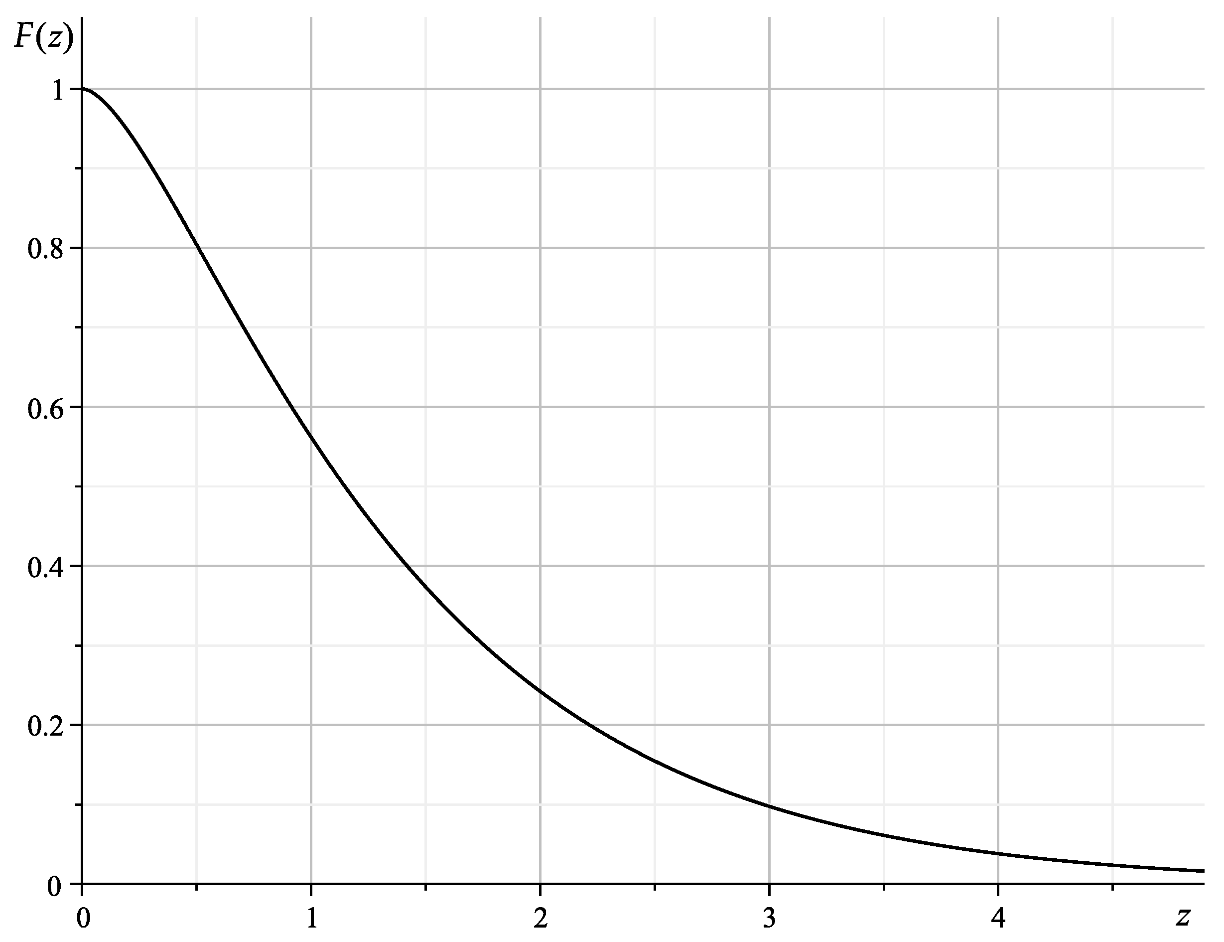
As a result, for $\mathcal{F}\left(z\right)$ one obtains eventually:

$$\begin{array}{c}\hfill \mathcal{F}\left(z\right)=\frac{z^2}{4}\left[\left(\frac{z^2}{6}-1\right)\left[K_0^2\left(\frac{z}{2}\right)-K_1^2\left(\frac{z}{2}\right)\right]+\left(\frac{z^2}{12}+1\right)zU\left(z\right)+\frac{z}{4}{K}_0\left(\frac{z}{2}\right)K_1\left(\frac{z}{2}\right)\right].\end{array}$$

(40)

The plot of $\mathcal{F}\left(z\right)$ is presented in Figure 2.

In what follows, for $z\gg 1$, the asymptotic expansion reads:

$$\mathcal{F}\left(z\right)=\frac{\pi }{16}{\mathrm{e}}^{-z}\left(15-\frac{75}{2z}+\frac{25,031}{128z^2}+\mathcal{O}\left(z^{-3}\right)\right).$$

Therefore, at large (with respect to the Compton length) distances, the Casimir effect is damped exponentially.

In the opposite case, for $z\ll 1$, the expansion is given by

$$\mathcal{F}\left(z\right)=1+\frac{5}{8}{z}^2\left(ln\frac{z}{4}+\gamma +\frac{1}{3}\right)+\mathcal{O}\left(z^4|lnz|\right),$$

and thus, one can see that for $d\ll l_c$, the contribution of massive modes into the Casimir energy turns out to be comparable to the contribution of massless modes, as follows from the qualitative speculations.

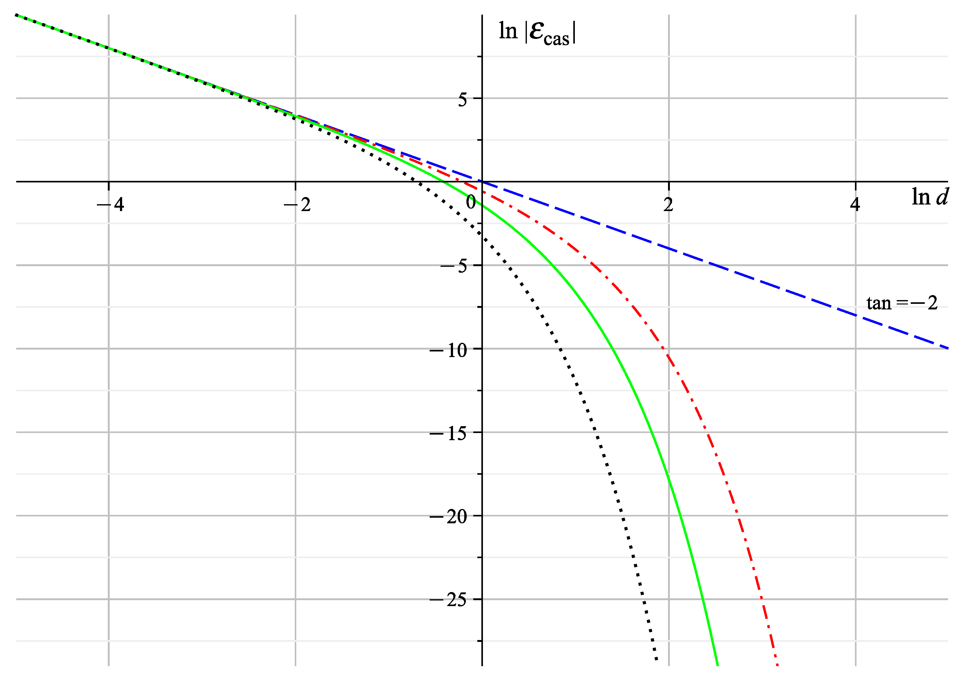
The plot of dependence of the Casimir energy,

$$\begin{array}{c}\hfill {\mathcal{E}}_{\mathrm{Cas}}=-\frac{4Z{\mu }_1{\mu }_2}{15d^2}\mathcal{F}\left(2md\right),\end{array}$$

(41)

as a function of interstring distance in doubly logarithmic scale is presented in Figure 3. The dashed line corresponds to the massless limit.

The corresponding attraction force per unit strings’ length is to be found as a derivative of the Casimir energy ${\mathcal{E}}_{\mathrm{Cas}}$ with respect to the strings-separation distance d. Therefore, both the Casimir energy and the Casimir force (both per unit length) are given by finite expressions.

5. Vacuum Interaction of Strings: $\mathbf{2}\mathit{a}<\mathit{d}\ll {\mathit{l}}_{\mathit{c}}$

As was noted in Section 1, the case $d\ll l_c$ corresponds to the observation that the field can be considered to be massless.

Then, returning to Equation (27) and fixing $m=0$, one obtains:

$$\begin{array}{c}\hfill {\mathcal{E}}_{\mathrm{vac}}^{\mathrm{ren}}=\frac{Z}{4{\left(4\pi \right)}^2}\int \frac{d^{2}k}{{\left(2\pi \right)}^2}\mathsf{\Lambda }\left(\mathit{k}\right)\mathsf{\Lambda }(-\mathit{k}){\mathit{k}}^4\underset{0}{\overset{1}{\int }}d\eta {\eta }^2{(1-\eta )}^{2}ln\frac{\eta (1-\eta ){\mathit{k}}^2}{{\tilde{\mu }}^2},\end{array}$$

(42)

and after the $\eta$-integration:

$$\begin{array}{c}\hfill {\mathcal{E}}_{\mathrm{vac}}^{\mathrm{ren}}=\frac{Z}{60{\left(4\pi \right)}^2}\int \frac{d^{2}k}{{\left(2\pi \right)}^2}\mathsf{\Lambda }\left(\mathit{k}\right)\mathsf{\Lambda }(-\mathit{k}){\mathit{k}}^4\left[ln\left|\mathit{k}\right|+\mathcal{O}\left(1\right)\right].\end{array}$$

(43)

Now after the substitution $\mathsf{\Lambda }\left(\mathit{k}\right)\to -\sigma \left(\mathit{k}\right)$ the expression (43) is rewritten as a sum of two integrals. One of them reads:

$$\begin{array}{c}\hfill \int \frac{d^{2}k}{{\left(2\pi \right)}^2}{\left|\mathit{k}\right|}^4\sigma \left(\mathit{k}\right)\sigma (-\mathit{k})=\int d^{2}x{\left[\Delta \sigma \left(\mathit{x}\right)\right]}^2\simeq \int d^{2}x{R}^2\left(\mathit{x}\right).\end{array}$$

(44)

The integral, which contains a logarithm in Equation (43), also can be transformed into the coordinate representation:

$$\begin{array}{cc}\hfill \int \frac{d^{2}k}{{\left(2\pi \right)}^2}{\left|\mathit{k}\right|}^{4}ln\left|\mathit{k}\right|\sigma \left(\mathit{k}\right)\sigma (-\mathit{k})& =-\frac{1}{2\pi }\int d^{2}x{d}^2{x}^{\prime }\frac{\Delta \sigma \left(\mathit{x}\right){\Delta }^{\prime }\sigma \left({\mathit{x}}^{\prime }\right)}{|\mathit{x}-{\mathit{x}}^{\prime }{|}^2}\hfill \\ & \simeq -\frac{1}{2\pi }\int d^{2}x{d}^2{x}^{\prime }\frac{R\left(\mathit{x}\right)R\left({\mathit{x}}^{\prime }\right)}{|\mathit{x}-{\mathit{x}}^{\prime }{|}^2}.\hfill \end{array}$$

(45)

In the expressions (44) and (45), it was taken into account that to the lowest order of $(1-\beta )$, which is of interest here,

$$\begin{array}{c}\hfill \Delta \sigma \left(\mathit{x}\right)=\sum _{\alpha }\Delta {\sigma }_{\alpha }\left(\mathit{x}\right)\simeq R\left(\mathit{x}\right)=\sum _{\alpha }{R}_{\alpha }\left(\mathit{x}\right).\end{array}$$

(46)

For two strings separated by distance $d>a_1+a_2$ ($\mathit{d}={\mathit{x}}_1-{\mathit{x}}_2$), the supports of the partial contributions $R_{\alpha }$ and $R_{\beta }$ do not overlap. Hence, that contribution to Equation (44), which depends upon the distance d, vanishes, and the Casimir contribution to the total vacuum energy (46) is completely determined by the contribution due to the integral (45). This contribution can be presented in the form

$$\begin{array}{c}\hfill {\mathcal{E}}_{\mathrm{Cas}}=-\frac{Z}{15{\left(4\pi \right)}^3}\underset{\begin{array}{c}\left|\mathit{x}\right|<a_1,\\ |{\mathit{x}}^{\prime }|<a_2\end{array}}{\int }{d}^{2}x{d}^2{x}^{\prime }\frac{R_1\left(\mathit{x}\right)R_2\left({\mathit{x}}^{\prime }\right)}{|\mathit{x}-{\mathit{x}}^{\prime }{+\mathit{d}|}^2}.\end{array}$$

(47)

Introduce two polar coordinate systems $(\varrho ,\phi )$ and $({\varrho }^{\prime },{\phi }^{\prime })$ (with suggestive notations) with origins in the centers of strings. Then, both angular integrations are carried out with the help of the table integral [33]

$$\begin{array}{c}\hfill \underset{0}{\overset{2\pi }{\int }}\frac{d\phi }{A+Bcos\phi }=\frac{2\pi }{\sqrt{A^2-B^2}}.\end{array}$$

It results in the following expression for the Casimir energy per unit length:

$$\begin{array}{c}\hfill \frac{{\mathcal{E}}_{\mathrm{Cas}}}{Z}=-\frac{16}{15\pi }\frac{{\mu }_1{\mu }_2}{a_1^2{a}_2^2}\underset{0}{\overset{a_1}{\int }}\varrho d\varrho \underset{0}{\overset{a_2}{\int }}\frac{{\varrho }^{\prime }d{\varrho }^{\prime }}{\sqrt{[{(d+{\varrho }^{\prime })}^2-{\varrho }^2][{(d-{\varrho }^{\prime })}^2-{\varrho }^2]}}.\end{array}$$

Integrating with respect to $\varrho$, one has:

$$\begin{array}{c}\hfill \frac{{\mathcal{E}}_{\mathrm{Cas}}}{Z}=-\frac{8}{15\pi }\frac{{\mu }_1{\mu }_2}{a_1^2{a}_2^2}\underset{0}{\overset{a_2}{\int }}{\varrho }^{\prime }d{\varrho }^{\prime }\left(ln\frac{d}{{\varrho }^{\prime }}-\mathrm{arccosh}\frac{d^2+{{\varrho }^{\prime }}^2-a_1^2}{2d{\varrho }^{\prime }}\right).\end{array}$$

(48)

The final integration yields:

$$\begin{array}{cc}\hfill \frac{{\mathcal{E}}_{\mathrm{Cas}}}{Z}=\frac{8}{15\pi }\frac{{\mu }_1{\mu }_2}{a_1^2{a}_2^2}& [\frac{d^2-2a_1^2}{8}-\frac{1}{8}\sqrt{{\left(d^2+a_1^2-a_2^2\right)}^2-4d^2{a}_1^2}+\hfill \\ & +\frac{a_1^2}{2}\left(\mathrm{arccosh}\frac{d^2+a_1^2-a_2^2}{2d{a}_1}-ln\frac{d}{a_1}\right)+\left\{a_1⟷a_2\right\}].\hfill \end{array}$$

(49)

In the case of GUT strings, both the mass per unit length and the string’s width are determined by the energy scale of the corresponding phase transition, ${\eta }_{\mathrm{GUT}}\sim {10}^{16}\mathrm{GeV}$. Hence it is reasonable to fix

$$a_1=a_2=a=a_{\mathrm{GUT}}\sim {\eta }_{\mathrm{GUT}}^{-1},{\mu }_1={\mu }_2=\mu ={\mu }_{\mathrm{GUT}}\sim {\eta }_{\mathrm{GUT}}^2$$

and consider two similar strings. Then, introducing

$$\xi =\frac{a}{d}<\frac{1}{2},$$

the energy of the Casimir attraction per unit length of two finite-width strings equals [34]

$$\begin{array}{c}\hfill \frac{{\mathcal{E}}_{\mathrm{Cas}}}{Z}=\frac{4}{15\pi }\frac{{\mu }^2}{d^2}\frac{1}{{\xi }^4}\underset{0}{\overset{{\xi }^2}{\int }}dxln\frac{1+x-{\xi }^2+\sqrt{{(1+x-{\xi }^2)}^2-4x}}{2}.\end{array}$$

(50)

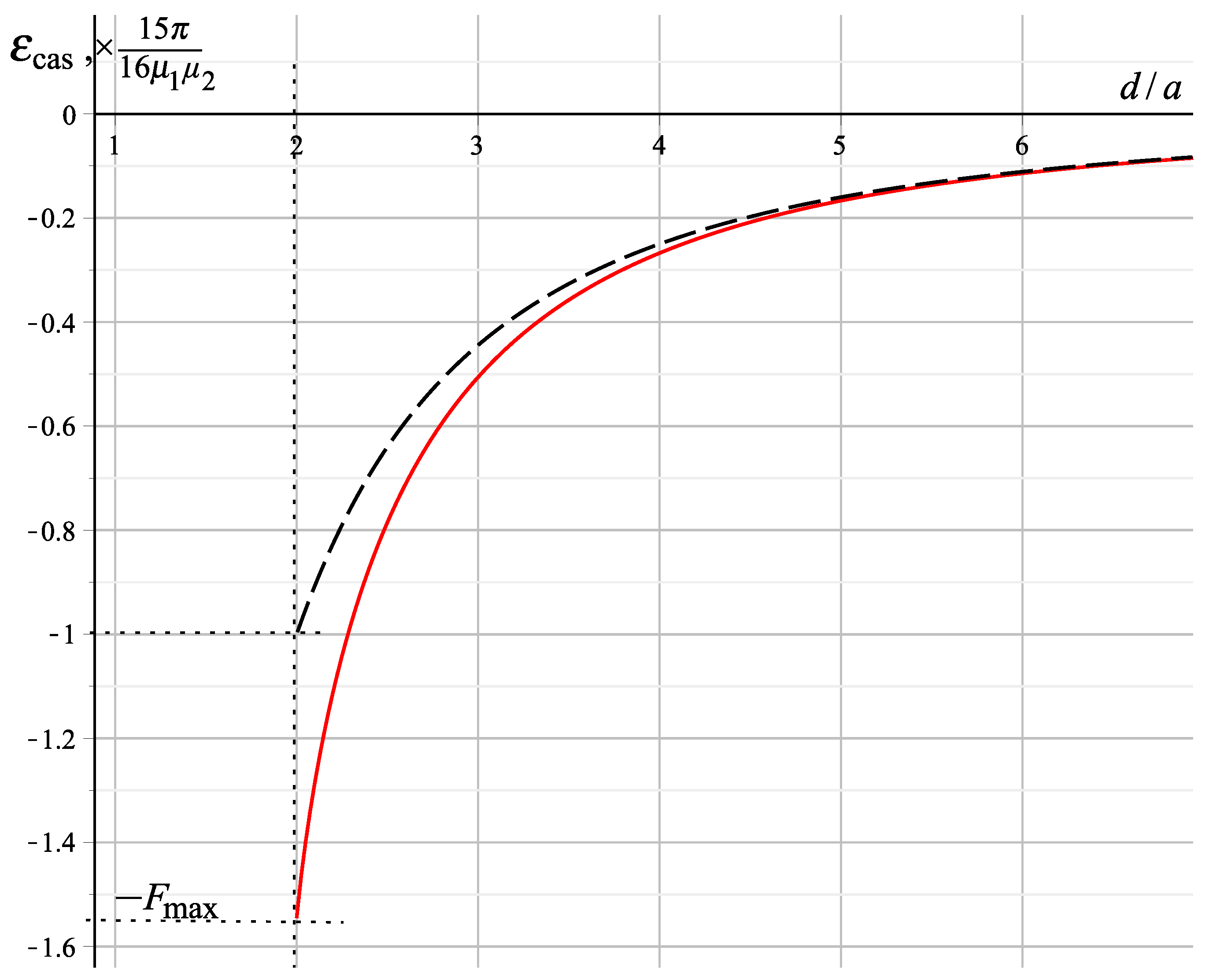
Finally, integrating with respect to x, the Casimir energy of two equivalent strings is given by

$$\begin{array}{c}\hfill \frac{{\mathcal{E}}_{\mathrm{Cas}}}{Z}=-\frac{4}{15\pi }\frac{{\mu }^2}{d^2}\frac{1}{{\xi }^2}\left[1-2ln\frac{1+\sqrt{1-4{\xi }^2}}{2}-\frac{1-\sqrt{1-4{\xi }^2}}{2{\xi }^2}\right].\end{array}$$

(51)

The dependence of the Casimir energy (normalized by $(-4{\mu }^2/15\pi )$) of attraction of two similar strings upon the interstring distance is plotted in Figure 4.

In the case $d\gg a$, the direct expansion in $\xi \ll 1$ yields

$$\begin{array}{c}\hfill \frac{{\mathcal{E}}_{\mathrm{Cas}}}{\mathrm{Z}}=-\frac{4}{15\pi }\frac{{\mu }^2}{d^2}\left[1+\frac{a^2}{d^2}+\frac{5}{3}\frac{a^4}{d^4}+\mathcal{O}\left(d^{-6}\right)\right],\end{array}$$

(52)

what to the leading (in $a/d$) order coincides with the result for infinitely thin strings [7,8,9].

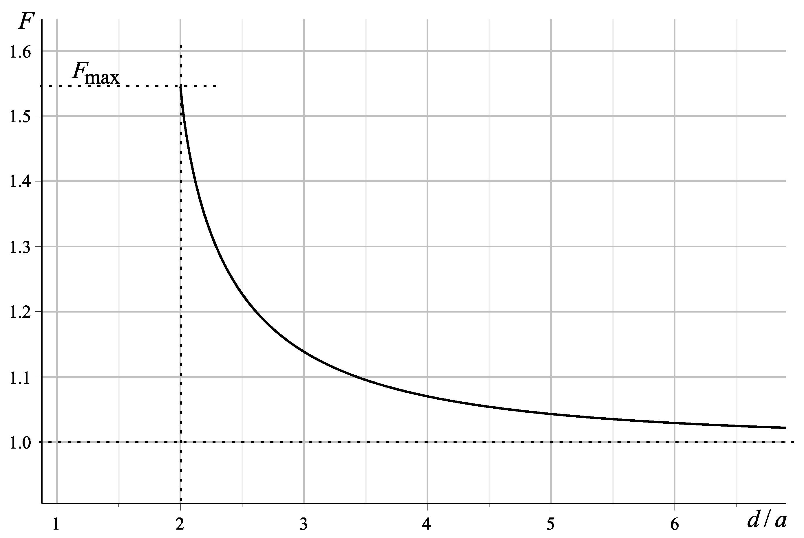
In Figure 5, we plot the curve of a ratio of the Casimir energy for the ballpoint-pen model with respect to the same quantity for infinitely thin strings.

Let us consider the case $a_1\ll a_2<d$ separately. It can be considered to be a case when one of the strings (namely, $a_2$) was formed under the electroweak (EW) phase transition. It happened with considerably lower energies $({\eta }_{\mathrm{EW}}\sim {10}^3\mathrm{GeV})$ and corresponds to the transverse size of the created strings of $a_{\mathrm{EW}}\sim {10}^{-15}\mathrm{cm}$, what significantly exceeds the corresponding width of a typical GUT-string $(a_{\mathrm{GUT}}\sim {10}^{-28}\mathrm{cm})$.

Then from the expression (48) we infer:

$$\begin{array}{c}\hfill \frac{{\mathcal{E}}_{\mathrm{Cas}}}{Z}=-\frac{8}{15\pi }\frac{{\mu }_1{\mu }_2}{a_2^2}\underset{0}{\overset{a_2}{\int }}\frac{{\varrho }^{\prime }d{\varrho }^{\prime }}{d^2-{{\varrho }^{\prime }}^2}+\mathcal{O}(a_1^2/d^2).\end{array}$$

(53)

In what follows, in the limit $a_1\to 0^{+}$, denoting $a_2=a$, one obtains

$$\begin{array}{c}\hfill \frac{{\mathcal{E}}_{\mathrm{Cas}}}{Z}=\frac{4}{15\pi }\frac{{\mu }_1{\mu }_2}{a^2}ln\left(1-\frac{a^2}{d^2}\right),\end{array}$$

(54)

so, for $d\gg a$, we return to the result valid for two infinitely thin strings.

However, in the case of close contact, where the interstring gap, $\delta =d-a$, is considerably smaller than the interstring distance d, Equation (54) gives logarithmic singularity (${\mathcal{E}}_{\mathrm{Cas}}\sim ln(2\delta /d)$) as ($\delta \to 0^{+}$). This implies that if $\delta$ becomes of the same order as the width of the thinner string, one cannot neglect string’s radius.

Let us demonstrate that under a contact of the strings of any finite width, the Casimir energy per unit length is finite within the model under interest. Then, two radii are related by $a_2=d-a_1$. Define $a=min\{a_1,a_2\}$ now and introduce $\overline{\xi }:=a/d$. Then for any $0<\overline{\xi }⩽1/2$,

$$\begin{array}{c}\hfill \frac{{\mathcal{E}}_{\mathrm{Cas}}}{Z}=-\frac{4}{15\pi }\frac{{\mu }_1{\mu }_2}{d^2}\frac{1}{{\overline{\xi }}^2}\left[\frac{{\overline{\xi }}^2(1-ln\overline{\xi })-\overline{\xi }}{{(1-\overline{\xi })}^2}-ln(1-\overline{\xi })\right].\end{array}$$

(55)

For $\overline{\xi }=1/2$ one reproduces the result (51) with $\xi =1/2$:

$$\begin{array}{c}\hfill \mathcal{F}=4(2ln2-1),\end{array}$$

(56)

while, in the opposite limiting case ($\overline{\xi }\ll 1$), the expansion in relatively small a reads:

$$\begin{array}{c}\hfill \frac{{\mathcal{E}}_{\mathrm{Cas}}}{Z}=-\frac{4}{15\pi }\frac{{\mu }_1{\mu }_2}{d^2}\left(ln\frac{d}{a}-\frac{1}{2}\right)+\mathcal{O}\left(a\right|lna\left|\right).\end{array}$$

(57)

From the quantitative viewpoint, this case (applied to the pair GUT-plus-EW strings) is of a significantly lower interest than the case of two similar GUT strings discussed in this Section. It happens since the energy per unit length, ${\mu }_{\mathrm{EW}}\sim {\eta }_{\mathrm{EW}}^2$, of the EW string is many orders smaller than the same energy, ${\mu }_{\mathrm{GUT}}$, for the GUT string. But from the qualitative viewpoint, for the EW strings, these effects take place already at the distances of the order of $d\sim 1/{\eta }_{\mathrm{EW}}\sim {10}^{-15}\mathrm{cm}$, in contrast to the orders ${10}^{-28}\mathrm{cm}$ for the Casimir interaction of two GUT strings. Also, the model considered above once again illustrates the nontrivial dependence of this effect on the strings’ size.

6. Discussion

We have presented an extended overview of recent results obtained by the authors in the process of studying the vacuum interaction of topological cosmic strings at short distances [34,35]. Within the tr-ln formalism, we have considered the vacuum interaction of finite-width topological cosmic strings, which interact via a massive scalar field with minimal coupling. It is shown that at distances much less than the Compton length but significantly larger than the strings’ width, the partial contribution of massive fields to the Casimir energy is comparable with the contribution of massless fields. Therefore, at such small (in the sense mentioned above) distances, one can neglect the mass. Nevertheless, if the interstring distance becomes comparable with the strings’ width, one cannot neglect the string radius. Furthermore, if the interstring gap is of the order of the string’s width, the energy of the Casimir interaction may significantly surpass the same quantity for the infinitely thin strings with the same mass per unit length.

The results obtained here may be useful in subsequent issues on the interaction of strings at short distances, on their collisions, and on accompanying intertanglements and reconnections.