Numerical Simulations of the Decaying Transverse Oscillations in the Cool Jet


Abstract
:1. Introduction
2. MHD Model of Cool Jets and Numerical Methods
2.1. The Ideal MHD System
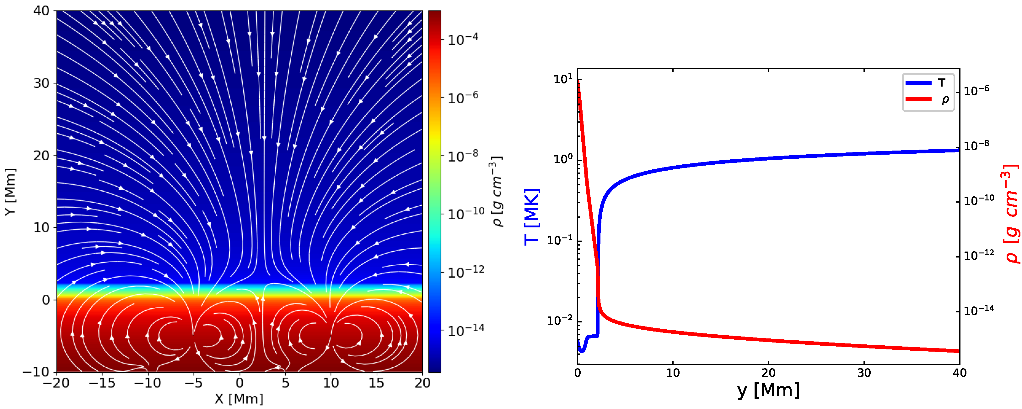
2.2. Equilibrium Condition of the Model Solar Atmosphere
2.3. Numerical Methods
2.4. Perturbation
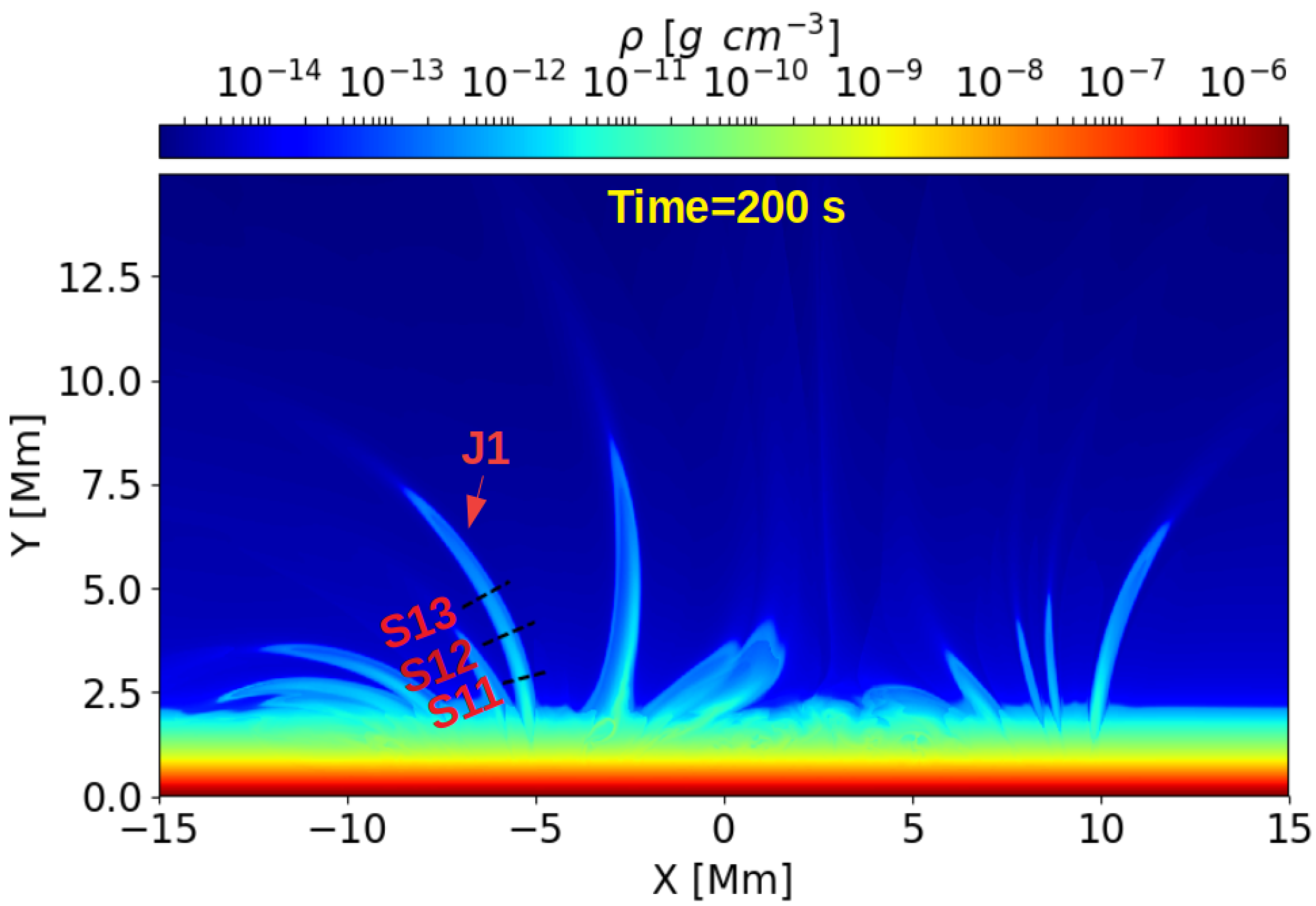
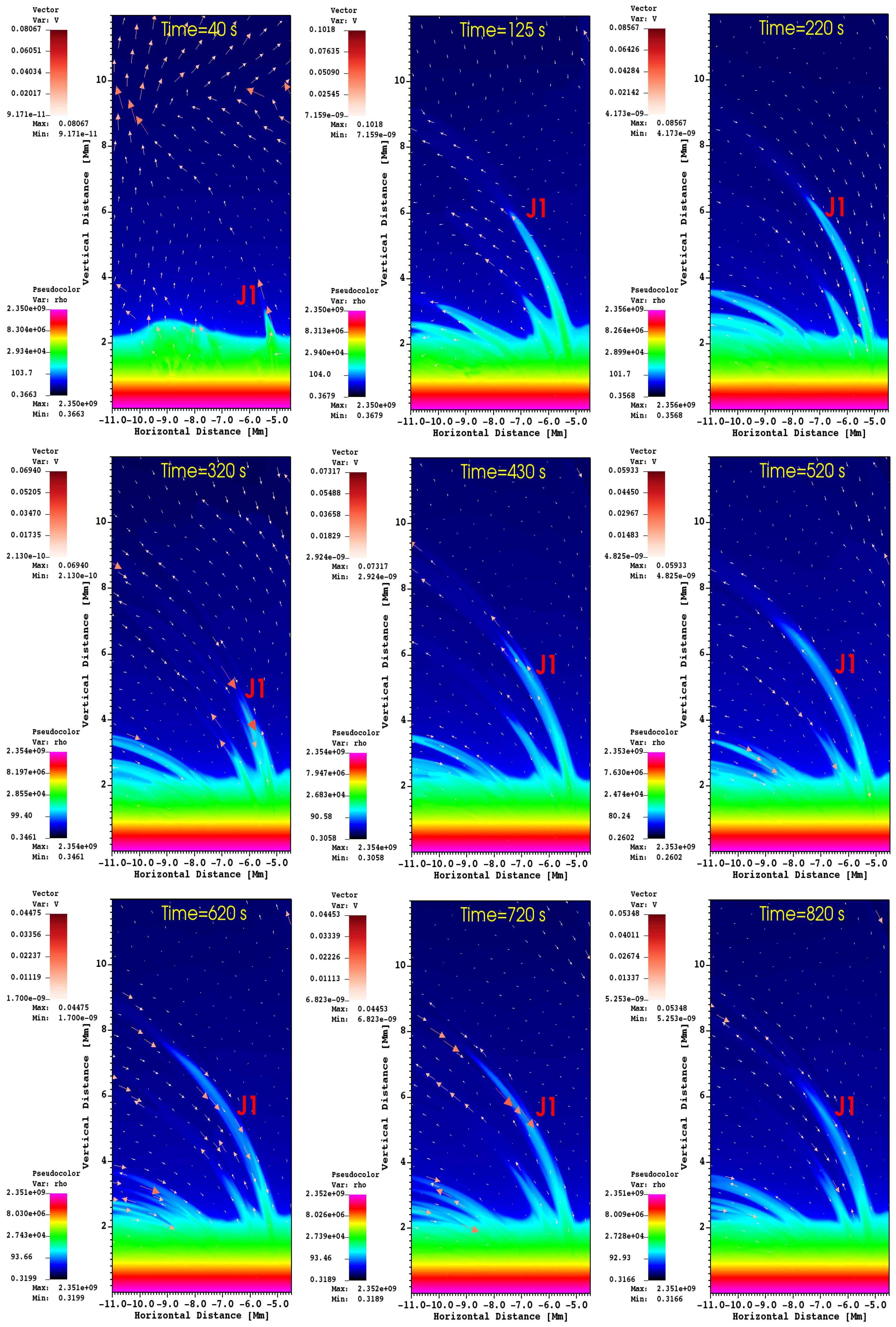
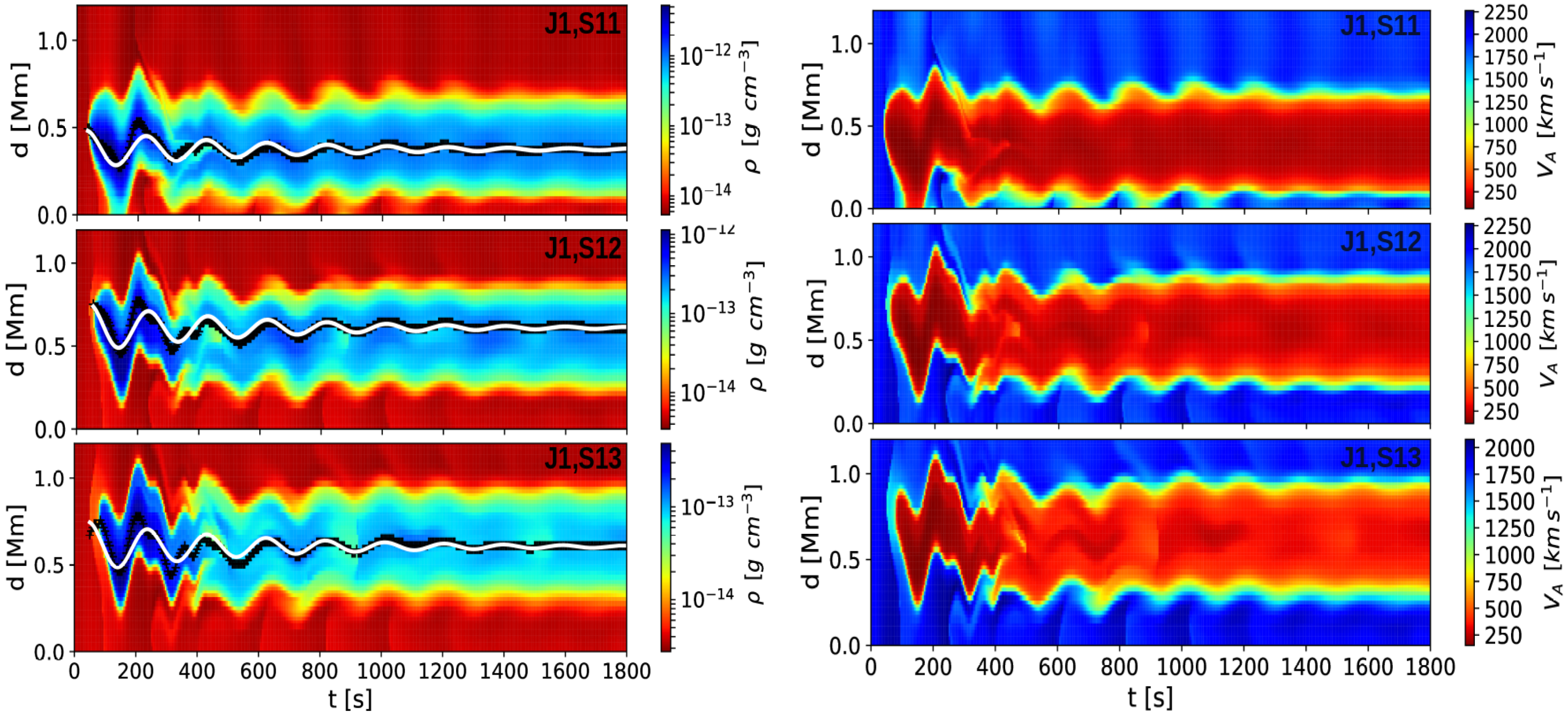
3. Results
4. Discussion and Conclusions
Supplementary Materials
Author Contributions
Funding
Data Availability Statement
Acknowledgments
Conflicts of Interest
References
- Sterling, A.C. Solar spicules: A review of recent models and targets for future observations. Sol. Phys. 2000, 196, 79–111. [Google Scholar] [CrossRef]
- De Pontieu, B.; Erdélyi, R.; James, S.P. Solar chromospheric spicules from the leakage of photospheric oscillations and flows. Nature 2004, 430, 536–539. [Google Scholar] [CrossRef] [PubMed]
- De Pontieu, B.; McIntosh, S.W.; Carlsson, M.; Hansteen, V.H.; Tarbell, T.D.; Schrijver, C.J.; Title, A.M.; Shine, R.A.; Tsuneta, S.; Katsukawa, Y.; et al. Chromospheric Alfvénic waves strong enough to power the solar wind. Science 2007, 318, 1574–1577. [Google Scholar] [CrossRef] [PubMed]
- Sterling, A.C.; Harra, L.K.; Moore, R.L. Fibrillar chromospheric spicule-like counterparts to an extreme-ultraviolet and soft X-ray blowout coronal jet. Astrophys. J. 2010, 722, 1644–1653. [Google Scholar] [CrossRef] [Green Version]
- McIntosh, S.W.; de Pontieu, B.; Carlsson, M.; Hansteen, V.; Boerner, P.; Goossens, M. Alfvénic waves with sufficient energy to power the quiet solar corona and fast solar wind. Nature 2011, 475, 477–480. [Google Scholar] [CrossRef]
- De Pontieu, B.; Rouppe van der Voort, L.; McIntosh, S.W.; Pereira, T.M.D.; Carlsson, M.; Hansteen, V.; Skogsrud, H.; Lemen, J.; Title, A.; Boerner, P.; et al. On the prevalence of small-scale twist in the solar chromosphere and transition region. Science 2014, 346, 1255732. [Google Scholar] [CrossRef] [Green Version]
- Jelínek, P.; Srivastava, A.K.; Murawski, K.; Kayshap, P.; Dwivedi, B.N. Spectroscopic observations and modelling of impulsive Alfvén waves along a polar coronal jet. Astron. Astrophys. 2015, 581, A131. [Google Scholar] [CrossRef] [Green Version]
- Srivastava, A.K.; Shetye, J.; Murawski, K.; Doyle, J.G.; Stangalini, M.; Scullion, E.; Ray, T.; Wójcik, D.P.; Dwivedi, B.N. High-frequency torsional Alfvén waves as an energy source for coronal heating. Sci. Rep. 2017, 7, 43147. [Google Scholar] [CrossRef]
- Liu, J.; Nelson, C.J.; Snow, B.; Wang, Y.; Erdélyi, R. Evidence of ubiquitous Alfvén pulses transporting energy from the photosphere to the upper chromosphere. Nat. Commun. 2019, 10, 3504. [Google Scholar] [CrossRef] [Green Version]
- Srivastava, A.K.; Murawski, K.; Kuźma, B.; Wójcik, D.P.; Zaqarashvili, T.V.; Stangalini, M.; Musielak, Z.E.; Doyle, J.G.; Kayshap, P.; Dwivedi, B.N. Confined pseudo-shocks as an energy source for the active solar corona. Nat. Astron. 2018, 2, 951–956. [Google Scholar] [CrossRef]
- Kayshap, P.; Murawski, K.; Srivastava, A.K.; Dwivedi, B.N. Rotating network jets in the quiet Sun as observed by IRIS. Astron. Astrophys. 2018, 616, A99. [Google Scholar] [CrossRef] [Green Version]
- Singh, B.; Sharma, K.; Srivastava, A.K. On modelling the kinematics and evolutionary properties of pressure-pulse-driven impulsive solar jets. Ann. Geophys. 2019, 37, 891–902. [Google Scholar] [CrossRef] [Green Version]
- Srivastava, A.K.; Rao, Y.K.; Konkol, P.; Murawski, K.; Mathioudakis, M.; Tiwari, S.K.; Scullion, E.; Doyle, J.G.; Dwivedi, B.N. Velocity response of the observed explosive events in the lower solar atmosphere. I. Formation of the flowing cool-loop system. Astrophys. J. 2020, 894, 155. [Google Scholar] [CrossRef]
- Panesar, N.K.; Tiwari, S.K.; Moore, R.L.; Sterling, A.C. Network jets as the driver of counter-streaming flows in a solar filament/filament channel. Astrophys. J. Lett. 2020, 897, L2. [Google Scholar] [CrossRef]
- Wang, Y.; Zhang, Q.; Ji, H. High-resolution He I 10830 Å narrowband imaging for a small-scale chromospheric jet. Astrophys. J. 2021, 913, 59. [Google Scholar] [CrossRef]
- Mackenzie Dover, F.; Sharma, R.; Erdélyi, R. Magnetohydrodynamic simulations of spicular jet propagation applied to lower solar atmosphere model. Astrophys. J. 2021, 913, 19. [Google Scholar] [CrossRef]
- Hou, Z.; Tian, H.; Berghmans, D.; Chen, H.; Teriaca, L.; Schühle, U.; Gao, Y.; Chen, Y.; He, J.; Wang, L.; et al. Coronal microjets in quiet-Sun regions observed with the extreme ultraviolet imager on board the solar orbiter. Astrophys. J. Lett. 2021, 918, L20. [Google Scholar] [CrossRef]
- Singh, B.; Srivastava, A.K.; Sharma, K.; Mishra, S.K.; Dwivedi, B.N. Quasi-periodic spicule-like cool jets driven by Alfvén pulses. Mon. Not. R. Astron. Soc. 2022, 511, 4134–4146. [Google Scholar] [CrossRef]
- Yuan, D.; Fu, L.; Cao, W.; Kuźma, B.; Geeraerts, M.; Trelles Arjona, J.C.; Murawski, K.; Van Doorsselaere, T.; Srivastava, A.K.; Miao, Y.; et al. Transverse oscillations and an energy source in a strongly magnetized sunspot. Nat. Astron, 2023; in print. [Google Scholar] [CrossRef]
- Tian, H.; DeLuca, E.E.; Cranmer, S.R.; De Pontieu, B.; Peter, H.; Martínez-Sykora, J.; Golub, L.; McKillop, S.; Reeves, K.K.; Miralles, M.P.; et al. Prevalence of small-scale jets from the networks of the solar transition region and chromosphere. Science 2014, 346, 1255711. [Google Scholar] [CrossRef] [Green Version]
- Samanta, T.; Tian, H.; Yurchyshyn, V.; Peter, H.; Cao, W.; Sterling, A.; Erdélyi, R.; Ahn, K.; Feng, S.; Utz, D.; et al. Generation of solar spicules and subsequent atmospheric heating. Science 2019, 366, 890–894. [Google Scholar] [CrossRef] [Green Version]
- Pasachoff, J.M.; Jacobson, W.A.; Sterling, A.C. Limb spicules from the ground and from space. Sol. Phys. 2009, 260, 59–82. [Google Scholar] [CrossRef]
- Takasao, S.; Isobe, H.; Shibata, K. Numerical simulations of solar chromospheric jets associated with emerging flux. Publ. Astron. Soc. Jpn. 2013, 65, 62. [Google Scholar] [CrossRef] [Green Version]
- Shibata, K.; Ishido, Y.; Acton, L.W.; Strong, K.T.; Hirayama, T.; Uchida, Y.; McAllister, A.H.; Matsumoto, R.; Tsuneta, S.; Shimizu, T.; et al. Observations of X-ray jets with the YOHKOH soft X-ray telescope. Publ. Astron. Soc. Jpn. 1992, 44, L173–L179. [Google Scholar] [CrossRef] [Green Version]
- Yokoyama, T.; Shibata, K. Magnetic reconnection as the origin of X-ray jets and Hα surges on the Sun. Nature 1995, 375, 42–44. [Google Scholar] [CrossRef]
- Heggland, L.; De Pontieu, B.; Hansteen, V.H. Numerical simulations of shock wave-driven chromospheric jets. Astrophys. J. 2007, 666, 1277–1283. [Google Scholar] [CrossRef] [Green Version]
- Nishizuka, N.; Shimizu, M.; Nakamura, T.; Otsuji, K.; Okamoto, T.J.; Katsukawa, Y.; Shibata, K. Giant chromospheric anemone jet observed with Hinode and comparison with magnetohydrodynamic simulations: Evidence of propagating Alfvén waves and magnetic reconnection. Astrophys. J. Lett. 2008, 683, L83–L86. [Google Scholar] [CrossRef] [Green Version]
- Murawski, K.; Zaqarashvili, T.V. Numerical simulations of spicule formation in the solar atmosphere. Astron. Astrophys. 2010, 519, A8. [Google Scholar] [CrossRef] [Green Version]
- Murawski, K.; Srivastava, A.K.; Zaqarashvili, T.V. Numerical simulations of solar macrospicules. Astron. Astrophys. 2011, 535, A58. [Google Scholar] [CrossRef] [Green Version]
- Kayshap, P.; Srivastava, A.K.; Murawski, K.; Tripathi, D. Origin of macrospicule and jet in Polar Corona by a small-scale kinked flux tube. Astrophys. J. Lett. 2013, 770, L3. [Google Scholar] [CrossRef] [Green Version]
- Iijima, H.; Yokoyama, T. A Three-dimensional magnetohydrodynamic simulation of the formation of solar chromospheric jets with twisted magnetic field lines. Astrophys. J. 2017, 848, 38. [Google Scholar] [CrossRef]
- Kuźma, B.; Murawski, K.; Kayshap, P.; Wójcik, D.; Srivastava, A.K.; Dwivedi, B.N. Two-fluid numerical simulations of solar spicules. Astrophys. J. 2017, 849, 78. [Google Scholar] [CrossRef] [Green Version]
- González-Avilés, J.J.; Murawski, K.; Srivastava, A.K.; Zaqarashvili, T.V.; González-Esparza, J.A. Numerical simulations of macrospicule jets under energy imbalance conditions in the solar atmosphere. Mon. Not. R. Astron. Soc. 2021, 505, 50–64. [Google Scholar] [CrossRef]
- Kuridze, D.; Morton, R.J.; Erdélyi, R.; Dorrian, G.D.; Mathioudakis, M.; Jess, D.B.; Keenan, F.P. Transverse oscillations in chromospheric mottles. Astrophys. J. 2012, 750, 51. [Google Scholar] [CrossRef]
- Morton, R.J. Magneto-seismological insights into the penumbral chromosphere and evidence for wave damping in spicules. Astron. Astrophys. 2014, 566, A90. [Google Scholar] [CrossRef]
- Tavabi, E.; Koutchmy, S. Oscillations in solar jets observed with the SOT of Hinode: Viscous effects during reconnection. Astrophys. Space Sci. 2014, 352, 7–15. [Google Scholar] [CrossRef] [Green Version]
- Pariat, E.; Dalmasse, K.; DeVore, C.R.; Antiochos, S.K.; Karpen, J.T. Model for straight and helical solar jets. I. Parametric studies of the magnetic field geometry. Astron. Astrophys. 2015, 573, A130. [Google Scholar] [CrossRef] [Green Version]
- Martínez-Sykora, J.; De Pontieu, B.; De Moortel, I.; Hansteen, V.H.; Carlsson, M. Impact of Type II spicules in the corona: Simulations and synthetic observables. Astrophys. J. 2018, 860, 116. [Google Scholar] [CrossRef] [Green Version]
- Srivastava, A.K.; Ballester, J.L.; Cally, P.S.; Carlsson, M.; Goossens, M.; Jess, D.B.; Khomenko, E.; Mathioudakis, M.; Murawski, K.; Zaqarashvili, T.V. Chromospheric heating by magnetohydrodynamic waves and instabilities. J. Geophys. Res. Space Phys. 2021, 126, e029097. [Google Scholar] [CrossRef]
- Kulidzanishvili, V.I.; Zhugzhda, I.D. On the problem of spicular oscillations. Sol. Phys. 1983, 88, 35–41. [Google Scholar] [CrossRef]
- Zaqarashvili, T.V.; Erdélyi, R. Oscillations and waves in solar spicules. Space Sci. Rev. 2009, 149, 355–388. [Google Scholar] [CrossRef] [Green Version]
- De Pontieu, B.; Erdélyi, R.; de Wijn, A.G. Intensity oscillations in the upper transition region above active region plage. Astrophys. J. Lett. 2003, 595, L63–L66. [Google Scholar] [CrossRef] [Green Version]
- Xia, L.D.; Popescu, M.D.; Doyle, J.G.; Giannikakis, J. Time series study of EUV spicules observed by SUMER/SoHO. Astron. Astrophys. 2005, 438, 1115–1122. [Google Scholar] [CrossRef]
- Pascoe, D.J.; Goddard, C.R.; Nisticò, G.; Anfinogentov, S.; Nakariakov, V.M. Damping profile of standing kink oscillations observed by SDO/AIA. Astron. Astrophys. 2016, 585, L6. [Google Scholar] [CrossRef] [Green Version]
- Kukhianidze, V.; Zaqarashvili, T.; Khutsishvili, E. Observation of kink waves in solar spicules. Astron. Astrophys. 2006, 449, L35–L38. [Google Scholar] [CrossRef]
- Jess, D.B.; Pascoe, D.J.; Christian, D.J.; Mathioudakis, M.; Keys, P.H.; Keenan, F.P. The origin of type I spicule oscillations. Astrophys. J. 2011, 744, L5. [Google Scholar] [CrossRef] [Green Version]
- Sarkar, S.; Pant, V.; Srivastava, A.K.; Banerjee, D. Transverse oscillations in a coronal loop triggered by a jet. Sol. Phys. 2016, 291, 3269–3288. [Google Scholar] [CrossRef] [Green Version]
- Zhang, Q.M.; Dai, J.; Xu, Z.; Li, D.; Lu, L.; Tam, K.V.; Xu, A.A. Transverse coronal loop oscillations excited by homologous circular-ribbon flares. Astron. Astrophys. 2020, 638, A32. [Google Scholar] [CrossRef]
- Dai, J.; Zhang, Q.M.; Su, Y.N.; Ji, H.S. Transverse oscillation of a coronal loop induced by a flare-related jet. Astron. Astrophys. 2021, 646, A12. [Google Scholar] [CrossRef]
- Nakariakov, V.M.; Anfinogentov, S.A.; Antolin, P.; Jain, R.; Kolotkov, D.Y.; Kupriyanova, E.G.; Li, D.; Magyar, N.; Nisticò, G.; Pascoe, D.J.; et al. Kink oscillations of coronal loops. Space Sci. Rev. 2021, 217, 73. [Google Scholar] [CrossRef]
- Zhang, Q.; Li, C.; Li, D.; Qiu, Y.; Zhang, Y.; Ni, Y. First detection of transverse vertical oscillation during the expansion of coronal loops. Astrophys. J. Lett. 2022, 937, L21. [Google Scholar] [CrossRef]
- Goossens, M.; Terradas, J.; Andries, J.; Arregui, I.; Ballester, J.L. On the nature of kink MHD waves in magnetic flux tubes. Astron. Astrophys. 2009, 503, 213–223. [Google Scholar] [CrossRef] [Green Version]
- Sterling, A.C.; Hollweg, J.V. The rebound shock model for solar spicules: Dynamics at long times. Astrophys. J. 1988, 327, 950–963. [Google Scholar] [CrossRef]
- Vranjes, J.; Pandey, B.P.; Poedts, S. Coupled gas acoustic and ion acoustic waves in weakly ionized plasma. Publ. Astron. Obs. Beograd 2008, 84, 507–510. Available online: https://ui.adsabs.harvard.edu/abs/2008POBeo..84..507V (accessed on 15 May 2023).
- Nakariakov, V.M.; Verwichte, E. Coronal waves and oscillations. Living Rev. Sol. Phys. 2005, 2, 3. [Google Scholar] [CrossRef] [Green Version]
- Goossens, M.; Andries, J.; Aschwanden, M.J. Coronal loop oscillations. An interpretation in terms of resonant absorption of quasi-mode kink oscillations. Astron. Astrophys. 2002, 394, L39–L42. [Google Scholar] [CrossRef] [Green Version]
- Goossens, M.; Andries, J.; Arregui, I. Damping of magnetohydrodynamic waves by resonant absorption in the solar atmosphere. Philos. Trans. R. Soc. Lond. Ser. A 2006, 364, 433–446. [Google Scholar] [CrossRef]
- Mignone, A.; Bodo, G.; Massaglia, S.; Matsakos, T.; Tesileanu, O.; Zanni, C.; Ferrari, A. PLUTO: A numerical code for computational astrophysics. Astrophys. J. Suppl. Ser. 2007, 170, 228–242. [Google Scholar] [CrossRef] [Green Version]
- Avrett, E.H.; Loeser, R. Models of the solar chromosphere and transition region from SUMER and HRTS observations: Formation of the extreme-ultraviolet spectrum of hydrogen, carbon, and oxygen. Astrophys. J. Suppl. Ser. 2008, 175, 229–276. [Google Scholar] [CrossRef] [Green Version]
- Low, B.C. Three-dimensional structures of magnetostatic atmospheres. I. Theory. Astrophys. J. 1985, 293, 31–43. [Google Scholar] [CrossRef]
- Wilhelm, K. Solar spicules and macrospicules observed by SUMER. Astron. Astrophys. 2000, 360, 351–362. [Google Scholar]
- Chae, J. Chromospheric magnetic reconnection. In New Solar Physics with Solar-B Mission; Shibata, K., Nagata, S., Sakurai, T., Eds.; Astronomical Society of the Pacific: San Francisco, CA, USA, 2007; pp. 243–255. Available online: https://ui.adsabs.harvard.edu/abs/2007ASPC..369..243C (accessed on 15 May 2023).
- Chen, Y.; Tian, H.; Huang, Z.; Peter, H.; Samanta, T. Investigating the transition region explosive events and their relationship to network jets. Astrophys. J. 2019, 873, 79. [Google Scholar] [CrossRef]
- Srivastava, A.K.; Singh, B.; Murawski, K.; Chen, Y.; Sharma, K.; Yuan, D.; Tiwari, S.K.; Mathioudakis, M. Impulsive origin of solar spicule-like jets. Eur. Phys. J. Plus 2023, 138, 209. [Google Scholar] [CrossRef]
- Edwin, P.M.; Roberts, B. Wave propagation in a magnetic cylinder. Sol. Phys. 1983, 88, 179–191. [Google Scholar] [CrossRef]
- Roberts, B. Waves and oscillations in the corona. Sol. Phys. 2000, 193, 139–152. [Google Scholar] [CrossRef]
- Goossens, M.; Erdélyi, R.; Ruderman, M.S. Resonant MHD waves in the solar atmosphere. Space Sci. Rev. 2011, 158, 289–338. [Google Scholar] [CrossRef]
- Shukhobodskiy, A.A.; Ruderman, M.S.; Erdélyi, R. Resonant damping of kink oscillations of thin cooling and expanding coronal magnetic loops. Astron. Astrophys. 2018, 619, A173. [Google Scholar] [CrossRef] [Green Version]
- Van Doorsselaere, T.; Gijsen, S.E.; Andries, J.; Verth, G. Energy propagation by transverse waves in multiple flux tube systems using filling factors. Astrophys. J. 2014, 795, 18. [Google Scholar] [CrossRef]
- Yu, D.J.; Van Doorsselaere, T. A Study on the excitation and resonant absorption of coronal loop kink oscillations. Astrophys. J. 2016, 831, 30. [Google Scholar] [CrossRef]
- Soler, R.; Ruderman, M.S.; Goossens, M. Damped kink oscillations of flowing prominence threads. Astron. Astrophys. 2012, 546, A82. [Google Scholar] [CrossRef]
- Zaqarashvili, T.V.; Khutsishvili, E.; Kukhianidze, V.; Ramishvili, G. Doppler-shift oscillations in solar spicules. Astron. Astrophys. 2007, 474, 627–632. [Google Scholar] [CrossRef] [Green Version]
- Sharma, R.; Verth, G.; Erdélyi, R. Evolution of complex 3D motions in spicules. Astrophys. J. 2018, 853, 61. [Google Scholar] [CrossRef] [Green Version]
- Shetye, J.; Verwichte, E.; Stangalini, M.; Doyle, J.G. The nature of high-frequency oscillations associated with short-lived spicule-type events. Astrophys. J. 2021, 921, 30. [Google Scholar] [CrossRef]
- Bate, W.; Jess, D.B.; Nakariakov, V.M.; Grant, S.D.T.; Jafarzadeh, S.; Stangalini, M.; Keys, P.H.; Christian, D.J.; Keenan, F.P. High-frequency waves in chromospheric spicules. Astrophys. J. 2022, 930, 129. [Google Scholar] [CrossRef]
- Ionson, J.A. Resonant absorption of Alfvénic surface waves and the heating of solar coronal loops. Astrophys. J. 1978, 226, 650–673. [Google Scholar] [CrossRef]
- Hollweg, J.V.; Yang, G. Resonance absorption of compressible magnetohydrodynamic waves at thin “surfaces”. J. Geophys. Res. Space Phys. 1988, 93, 5423–5436. [Google Scholar] [CrossRef]
- Sakurai, T.; Goossens, M.; Hollweg, J.V. Resonant behaviour of magnetohydrodynamic waves on magnetic flux tubes. I. Connection formulae at the resonant surfaces. Sol. Phys. 1991, 133, 227–245. [Google Scholar] [CrossRef]
- Goossens, M.; Hollweg, J.V.; Sakurai, T. Resonant behaviour of magnetohydrodynamic waves on magnetic flux tubes. III. Effect of equilibrium flow. Sol. Phys. 1992, 138, 233–255. [Google Scholar] [CrossRef]
- Aschwanden, M.J. Physics of the Solar Corona. An Introduction; Praxis Publishing Ltd.: Chichester, UK; Springer: Berlin/Heidelberg, Germany, 2004. [Google Scholar]
- Martínez-Sykora, J.; De Pontieu, B.; Hansteen, V.H.; Rouppe van der Voort, L.; Carlsson, M.; Pereira, T.M.D. On the generation of solar spicules and Alfvénic waves. Science 2017, 356, 1269–1272. [Google Scholar] [CrossRef] [Green Version]
- Hollweg, J.V.; Jackson, S.; Galloway, D. Alfven waves in the solar atmospheres. III. Nonlinear waves on open flux tubes. Sol. Phys. 1982, 75, 35–61. [Google Scholar] [CrossRef]
- Kudoh, T.; Shibata, K. Alfvén wave model of spicules and coronal heating. Astrophys. J. 1999, 514, 493–505. [Google Scholar] [CrossRef]
- Brady, C.S.; Arber, T.D. Simulations of Alfvén and kink wave driving of the solar chromosphere: Efficient heating and spicule launching. Astrophys. J. 2016, 829, 80. [Google Scholar] [CrossRef] [Green Version]


| Jet | Slit | A (Mm) | β (s−1) | ω (rad s−1) | ϕ (rad) |
|---|---|---|---|---|---|
| J1 | S11 | 0.1143 ± 0.0067 | 0.0018 ± 0.0001 | 0.0318 ± 0.0001 | −0.95857 ± 0.0582 |
| S12 | 0.1557 ± 0.0099 | 0.0018 ± 0.0001 | 0.0323 ± 0.0001 | −1.3568 ± 0.0596 | |
| S13 | 0.1545 ± 0.0117 | 0.0018 ± 0.0002 | 0.0325 ± 0.0002 | −1.4839 ± 0.0729 |
Disclaimer/Publisher’s Note: The statements, opinions and data contained in all publications are solely those of the individual author(s) and contributor(s) and not of MDPI and/or the editor(s). MDPI and/or the editor(s) disclaim responsibility for any injury to people or property resulting from any ideas, methods, instructions or products referred to in the content. |
© 2023 by the authors. Licensee MDPI, Basel, Switzerland. This article is an open access article distributed under the terms and conditions of the Creative Commons Attribution (CC BY) license (https://creativecommons.org/licenses/by/4.0/).
Share and Cite
Srivastava, A.K.; Singh, B. Numerical Simulations of the Decaying Transverse Oscillations in the Cool Jet. Physics 2023, 5, 655-671. https://doi.org/10.3390/physics5030043
Srivastava AK, Singh B. Numerical Simulations of the Decaying Transverse Oscillations in the Cool Jet. Physics. 2023; 5(3):655-671. https://doi.org/10.3390/physics5030043
Chicago/Turabian StyleSrivastava, Abhishek K., and Balveer Singh. 2023. "Numerical Simulations of the Decaying Transverse Oscillations in the Cool Jet" Physics 5, no. 3: 655-671. https://doi.org/10.3390/physics5030043