1. Introduction
Living in the era of the LHC (Large Hadron Collider), one has access to an unprecedentedly huge amount of data recorded by the state-of-the-art experimental facilities. Many intriguing results have been obtained for both proton–proton and ion–ion collisions that require a deep perception from the theoretical point of view. For example, the two most-significant ones are (i) the appearance of a so-called ridge phenomena in proton-proton (pp) collisions at the LHC—the long-range rapidity structure [
1]—and (ii) the onset of collectivity in small systems [
2].
Since the calculations from the first principles are often not possible in the theory of strong interactions and in the QCD (quantum chromodynamics), then the most-popular way to understand the experimental results is to compare them to simulations performed with some widely used Monte Carlo event generators. They usually contain many versions and tunes, including various options for some physical processes to be selected to be switched on and off.
In this study, we probe the sensitivity of different experimental observables to the details of the particle source formation in 3D (three-dimensional) dynamics to see a particular effect of one or another model’s features on the final correlation measures.
We focus on the modelling of initial-state configurations of pp collisions, and we attempt to mimic soft processes that result in multiparticle production. To implement this, we follow the philosophy of the phenomenological colour string model that was initially based on the two-stage particle production scenario [
3]. In the first stage, the longitudinally extended tubes of colour flux, so-called quark–gluon strings, are formed between wounded partons of the colliding hadrons. In the second stage, strings fragment into hadrons via the colour vacuum break-down because of the creation of quark–antiquark pairs. Therefore, in this framework, one naturally accounts for the initial conditions of hadronic collision via the quark–gluon string kinematics. The effective string breaking results later in the production of observed particles.
What in principle differentiates our Monte Carlo model from the aforementioned event generators and from the original string model approach is the mechanism of the string–string interaction taken in the form of the so-called string fusion [
4]. In the case of the absence of any interactions, the factorisation occurs, and the resulting spectra can be considered as a convolution of the spectra originating from the independent strings and of the distribution in several stretched strings. In the case of a high density of strings formed, the interactions between the strings as a fusion will increase the colour field density inside the new colour flux tubes formed. This changes the strings’ characteristics, which affects the particle production.
In this paper, we argue that not only string fusion plays an important role at the initial stages, but another peculiarity, the consideration of the detailed dynamics of strings’ formation is essential. The latter complicates the inner structure of the model and deprives it of the translational invariance in the rapidity. Thus, the model is a powerful tool for studying long-range rapidity correlations, and in combination with the string fusion effect, it may serve to study different types of particle production sources.
The main object is to quantify the long-range correlations between some observables measured event-by-event in pp collisions in two separate pseudorapidity intervals that are usually selected symmetrically with respect to the midrapidity. Based on the causality principle, it was shown in Ref. [
5] that, if the long-range rapidity correlation between particles exists, then the correlation must be formed at a proper and very early stage of collision. Therefore, in this study, we concentrate on the long-range rapidity correlations, as we are most interested in the role of the initial conditions and the sensitivity to the details of the evolution of the colliding system.
In this paper, the event-by-event fluctuations in the number of particle-emitting sources are for brevity called “volume” fluctuations. This reflects our approach to the study of the initial states of a system that has a complex spatial structure. We consider the so-called strongly intensive observable, , which suppresses these trivial fluctuations. In addition, we look at the event asymmetry coefficient that reflects the asymmetrical distribution of the particle sources (strings and string clusters) in rapidity, which results in the forward–backward correlations as well.
In the present study, the resonance decays, jets, and other particle production mechanisms characterised by short-range correlations are not considered. This is because of the main interest in the search for observables being related to the string fusion phenomena and the appearance of long-range rapidity correlations measured in hadron collisions in well-separated forward and backward rapidity intervals (about a unit of rapidity). Moreover, as soon as we study soft processes of particle production, i.e., non-perturbative effects, the main role is played by the hadrons with the transverse momentum, , up to 1.5–2 GeV/ (with c the speed of light), and our model does not include the simulation of hard processes.
The paper is organized as follows. In
Section 2, we briefly present the developed model and describe its key features and parameters. In this Section, we introduce the longitudinal and transverse dynamics of strings and describe the mechanism of their fusion. In
Section 3, we perform the fits to the global observables and spectra, i.e., we explain how the parameters listed in
Section 2 are obtained. Further, in
Section 3, we present the model predictions for the forward–backward rapidity correlations measured with the correlation coefficient, the strongly intensive quantity,
, and the “almost” strongly intensive observable,
, where
C is the event-by-event asymmetry coefficient of the multiplicity distribution in rapidity. In addition, we show the connection of
with such quantities like the often used cumulants and factorial cumulants. We also obtain the dependence of
on the selected forward-multiplicity-based classes. Finally, in
Section 4, we discuss the results obtained.
2. Definitions and Model
In the model considered here, we assume an inelastic collision of two protons (called an event).
2.1. Multi-Pomeron Exchange in pp Collisions
The number of strings,
, formed in the pp-collision event comes from the pomeron number,
, distribution [
6] as
. This is due to the mechanism, in which colour strings appear from the unitarity cut of a cylindrical pomeron exchange diagram [
7], while without the cut, the diagram represents an elastic scattering. We sample
from
where
,
is the quasi-eikonal parameter related to the small-mass diffraction dissociation of incoming hadrons,
is the residue of the pomeron trajectory,
and
characterise the coupling of the pomeron trajectory with the initial hadrons, the slope of the pomeron trajectory
,
s is the square of the collision centre-of-mass energy, and
is a normalising coefficient.
The values of these parameters are taken from Ref. [
8], where one assumes that the number of primary strings in an event (related to
from Equation (
1)) is initially formed, and then, some of them can fuse, forming the string clusters with the modified fragmentation characteristics. This framework can be viewed as a three-step scenario: first, strings are produced; then, they interact (fusion); lastly, the strings hadronisation occurs.
One may note that this is in contrast to another approach used in Ref. [
9], where the strings were considered to be produced of different types from the very beginning, so that the string fusion was effectively implemented already at the string formation moment. These two methods will necessarily differ in the values of the parameters in Equation (
1) so that the final charged particle multiplicity distribution,
(
2), describes the data. However, the present scenario allows us to introduce the 3D dynamics of string formation and evolution. Formally, in our approach,
although the exact form of
is unknown because of the complexity of an event picture in our model of interacting strings of different lengths and positions in the rapidity space; thus, we treat
within a Monte Carlo simulation.
The mechanism of pp collision is described as a multi-pomeron exchange, and we consider only strings stretched between quarks and anti-quarks of the colliding protons (no diquarks as string end-points were implemented). Taking this into account, we suppose that the number of partons in each of the colliding protons is equal to the number of strings per event.
2.2. Event-by-Event Sets of Protons and Parton’s Permutations
The problem to solve is that for every collision event, characterised by a certain number of exchanged pomerons, one has to form two protons with a given number of partons. Besides, on the one hand, it is necessary, to respect the energy and momentum conservation laws and, on the other hand, not to spoil the parton distribution functions. To meet these requirements in the Monte Carlo simulation, we propose to use the following algorithm of partons’ permutations.
First, one prepares extensive sets of protons for each possible number of partons. Each parton momentum is sampled as proton momentum fraction,
(where
i denotes the
ith parton), according to the parton distribution functions (PDFs) from CT10nnlo, next-to-next-to-leading order approximation [
10], by the CTEQ (Coordinate Theoretical-Experimental Project on QCD) group based on CT10 PDFs [
11], set 1, of LHAPDF (Les Houches Accord Parton Density Functions) [
12] at the momentum transferred,
(GeV/
c)
. A parton is assigned with the current quark mass of a certain flavour that is found from the probability distribution for a given
. At this point, there is no restriction to the parton content in terms of
.
Second, the generated partons are rearranged between protons in order to have and for all protons, where , is a mass of the ith parton, is the mass of the proton, and is the proton beam rapidity, .
Thus, it is ensured that the total energy and momenta of the partons are equal to the proton’s energy and momentum. To perform this, two protons (necessarily with the same number of partons) are selected and two randomly chosen partons, one taken from each proton, are exchanged between them. This permutation is accepted only if such a rearrangement decreases and (if the sums are larger than 1 in the previous step) or increases and (if the sums are smaller than 1 in the previous step) simultaneously for both considered protons.
The computation time of such an algorithm grows crucially with the number of considered partons. Therefore, one actually cannot reach exactly the value of 1 for and . Thus, the permutations stop at some reasonable number of iterations (i.e., when the improvement caused by the exchange of the pair of partons becomes negligible), which leads to the lack of and compared to 1. Therefore, to compensate, an object called a gluon cloud with the momentum fraction, and is introduced. It is assigned the mass, , with the energy and the momentum of the gluon cloud, and is considered a parton that later is also used to form strings.
Finally, a string is stretched between two randomly selected partons belonging to two randomly selected protons (but with the same number of partons). A string is accepted only if its energy is sufficient to decay at least into two pions at rest meaning that
[
13] with
denoting the pion mass. Thus, all partons from the two colliding protons should form such strings. Otherwise, another random proton pair to be sought.
2.3. Strings Motion in Transverse Plane
Initial transverse positions of the strings are sampled from the Gaussian distribution respecting the cross-section area of a proton. Then, the strings are put in motion in the transverse plane according to the system of differential equations of the second order,
defined by the two-dimensional Yukawa interaction [
14]. Here,
is a 2D distance between the
ith and
jth strings,
is a regularized 2D distance in which there is no Coulomb singularity at small
due to the introduction of
fm [
14] that is a genuine string width, unlike the effective string width, which is a result of quantum fluctuations;
is the QCD string self-interaction coupling [
15];
GeV/
c [
14] is the mass of the
-meson that is a mediator of the force between strings;
is a modified Bessel function due to the cylindrical symmetry of the problem. Following Equation (
3), strings are considered moving as a whole, with no kinks.
It is worth mentioning that, in the case of many overlapping strings, their interaction will lead to the formation of string clusters, which at some threshold, eventually may cause the quark–gluon plasma formation. That is to say that some density of overlapping strings will be sufficient to eliminate the quark-antiquark chiral condensate,
, because of its suppression in the vicinity of colour strings [
14], which will lead to the restoration of the chiral symmetry.
Transverse strings’ evolution governed by Equation (
3) can be terminated at some proper time,
, which will affect the final string density. We consider two scenarios. In the first scenario, the system of strings is frozen at some conventional time (same for all events) before the start of string fragmentation at
fm/
c [
14]. In the second case, the system is fixed at
time, obtained event-by-event. This is the time that takes for some initial configuration of strings in the transverse plane to reach the global minimum of the potential energy, changing according to Equation (
3). Thus,
depends not only on the initial string transverse positions, but also on the number of strings, hence on the collision energy. It is also worth emphasising that, for
fm/
c, one obtains a more dilute system, while for
, the string density is highest.
2.4. Strings’ Longitudinal Evolution
In the longitudinal direction, initial strings’ end rapidities, defined by partons forming a string and expressed by the first term in
are decreased [
16] by the loss of string length in rapidity,
, expressed by the second term in Equation (
4). It is the string tension
that slows down the massive quarks flying outwards according to
, where
is a proton beam momentum,
is the square of the collision centre-of-mass energy per nucleon pair,
GeV/
c,
is a current quark mass (we consider
GeV/
c,
GeV/
c,
GeV/
c, and
GeV/
c for
u,
d,
s, and
c quarks, respectively) or
.
Note that here is the same time as for the transverse dynamics; therefore, string evolution is synchronised in both dimensions.
An important remark is that the value of the evolution time changes not only the length of the strings, but also strings’ positions with respect to midrapidity. This is because
(the second term in Equation (
4)) applies to both ends of the string and depends on the quark’s mass and momentum. Therefore, some strings can even lie entirely in one hemisphere if
is large enough such that the second term in Equation (
4) is greater than the first term in absolute value.
2.5. String Fusion
Considering strings density evolution in the rapidity and transverse plane dimensions, we study the fusion of strings in the string’s final configuration. Having a finite size in the transverse plane caused by the colour confinement, strings may overlap with the different degrees of intersection.
As a reference scenario to string fusion, we consider the case of independent sources, so, at this step, the possibility of strings interacting is ignored, even when overlapped.
Our main interest here is to consider string–string interaction effects in a form of fusion leading to a new type of string with higher tension. There are several options on how to account for this; see [
17] for corresponding studies.
First, one may assume that the colour field changes only in the areas where strings overlap and stays the same in the rest of the transverse strings’ area. Another possibility is that, if strings overlap, even on an arbitrarily small area, the strings form a cluster, which has the uniformly modified colour field on the area of the union of all these strings. However, so far, the attempts were in vain to find the observables sensitive to the type of overlap mode. Therefore, we follow a cellular approach in the transverse plane developed in Ref. [
17]. This means that we only look after strings’ centre position on the transverse grid with the constant cell size, which reflects the string transverse area. Thereby, the only strings to interact are the strings whose centres lie in the same transverse cell. This simplification is beneficial from the point of view of computing resources, and besides, it gives the same results as a full-scale simulation that should account for the particular areas of overlap.
One has to mention that the fusion problem becomes three-dimensional since in the rapidity space there are the fluctuations of both the lengths of strings and the strings’ positions with respect to midrapidity. Thus, for strings occupying the same cell in the transverse plane, one has to search for their overlaps in the rapidity space to perform fusion in slices in rapidity.
Technically,
k overlapping strings that have centres in some transverse cell and overlap over some rapidity interval are replaced by a cluster of
k strings, which can be seen as a new string with the modified particle production characteristics [
18]:
while
is the mean particle multiplicity per rapidity unit for an independent string. The parts of the initial strings that do not overlap in the rapidity space (even though string centres may lie in the same transverse cell) maintain the same colour field characteristics, and are considered also as separate strings. Thus, the process of string fusion makes overlapping strings shorter in the rapidity space, although the strings obtain the modification factor
k as stated in Equation (
5), which results in an overall decrease of mean multiplicity for interacting sources.
One can qualitatively explain Equation (
5) as follows. Given the case of the overlap of a few strings, their colour field vectors could be randomly oriented with respect to each other. To find the total colour field inside the cluster of overlapping strings, one can consider this problem as a random walk in the vector colour space, thus giving not the factor of
k, but
for
k overlapping strings compared to a single independent string. The first consideration of this behaviour was proposed in Ref. [
19], while a rigorous comparison of the string percolation approach to the colour–glass condensate model can be found in Ref. [
20].
The modification of the transverse momentum,
, spectrum was supposed [
21] to be performed according to the mean,
, where
stands for the mean transverse momentum of particles produced by independent sources. Thus, strings’ interaction causes the increase in particle mean-
. However, in Refs. [
9,
22], instead
is made dependent on the total number,
M, of strings in an event as power,
. The
depends on the collision energy, and for LHC energies,
. This gives us the idea to combine these two approaches and to introduce the factor
instead of
. However, let us stress that the
k here is a number of strings in a string cluster in some rapidity interval in some transverse cell, while
M from Refs. [
9,
22] is the overall number of particle sources in an event. Eventually, we apply the following modification for the mean-
from a cluster:
which would be of special interest in our future studies of pp interactions at lower collision energies, where
changes sign according to the fit in Ref. [
22].
In the current implementation of the model, at this moment of simulation, the string system is already frozen, and no transverse position is assigned to the cluster of strings (new strings), as soon as there is no need of it in the further calculations. However, one can introduce the transverse position as an average value over transverse positions of k fused strings.
Thus, after the initial strings’ dynamics in transverse and longitudinal spaces is considered and after the string fusion procedure is completed, one has a mixture of particle production sources: (i) strings (or parts of strings in rapidity) that did not undergo the process of fusion (let us call them single strings) so that one has to use for them
in Equations (
5) and (
6) and (ii) new strings (which we call clusters of strings) with
, 3, or other values in Equations (
5) and (
6) that reflect the degree of the strings’ overlap for these clusters.
2.6. Effective String Hadronisation
We perform effective string hadronisation by dividing the string in the
y-direction into units of length,
, to relate particles’ rapidities with the corresponding pieces of strings. This gives the mean multiplicity,
, for
unit and the actual multiplicity,
, sampled from the Poisson distribution with the mean
. Thus, multiplicity from the
jth string in an event is the sum of its
pieces:
, and event multiplicity is the sum over multiplicities from all strings in event:
. Particles’ rapidities are sampled from the Gauss distribution for each
unit with the mean equal to the centre of the
unit and with variance equal to
. It is important to mention that this
-division is only a technical solution to approximate the string fragmentation. Therefore, this procedure is the same for the single strings and clusters of strings. The substantial changes when considering string fusion appear in the factor
k for mean multiplicities (
5) and mean transverse momenta (
6), as well as for the Schwinger-like probabilities for the production of particle species.
Particles’ transverse momentum is sampled from the distribution,
which corresponds to the Schwinger mechanism of particle production [
23,
24,
25], with
from Equation (
6). Here, particle species,
i, are assigned according to Schwinger-like probabilities,
, which is consistent with Equation (
7), since we set
. In the model, we consider
,
K, and
p particles and
-resonance, with the latter decaying into two charged pions. With particle masses, the longitudinal component of momentum,
, is found and, thus, the pseudorapidity,
is calculated for each particle, where
is an absolute value of particle total momentum.
2.7. Model Tuning
To tune our model, we simultaneously fit the ALICE experiment pp inelastic interaction data at
GeV on the charged particle multiplicity distribution,
-spectrum [
26], and
–
N correlation function [
27], where the
denote the averaging over events. Global model parameters not affecting the result are: the hadronisation parameter,
and the transverse grid cell size of 0.3 fm. The best fit results are obtained for the model free parameters
and
GeV/
c. The values of the parameters for multi-pomeron distribution and for the transverse dynamics of strings are fixed to those from
Section 2.1,
Section 2.2,
Section 2.3,
Section 2.4 and
Section 2.5.
3. Results
We consider a few cases of the evolution of strings’ system:
no transverse string dynamics, but for longitudinal dynamics fm/c is used;
both the transverse and longitudinal string dynamics occur till fm/c;
both the transverse and longitudinal dynamics occur till (which changes event to event depending on the initial string configuration in the transverse plane).
For each of the above cases, the results are compared for independent and interacting sources, as the evolution time determined the three-dimensional event string density, which stimulated string fusion.
The model results for different sets of string dynamics parameters are compared with PYTHIA8.3 Monte Carlo generator simulations [
28] with a default list of settings (the Monash pp tune for non-diffractive events), which are also plotted with the colour reconnection option switched off and on. A qualitative comparison with the ALICE data on pp collisions at
GeV is also performed.
3.1. Global Observables
Starting from quite a complicated string structure in the rapidity space (strings’ lengths and positions of strings’ ends significantly vary event-by-event), a symmetrical inclusive -distribution is obtained in the whole available -range.
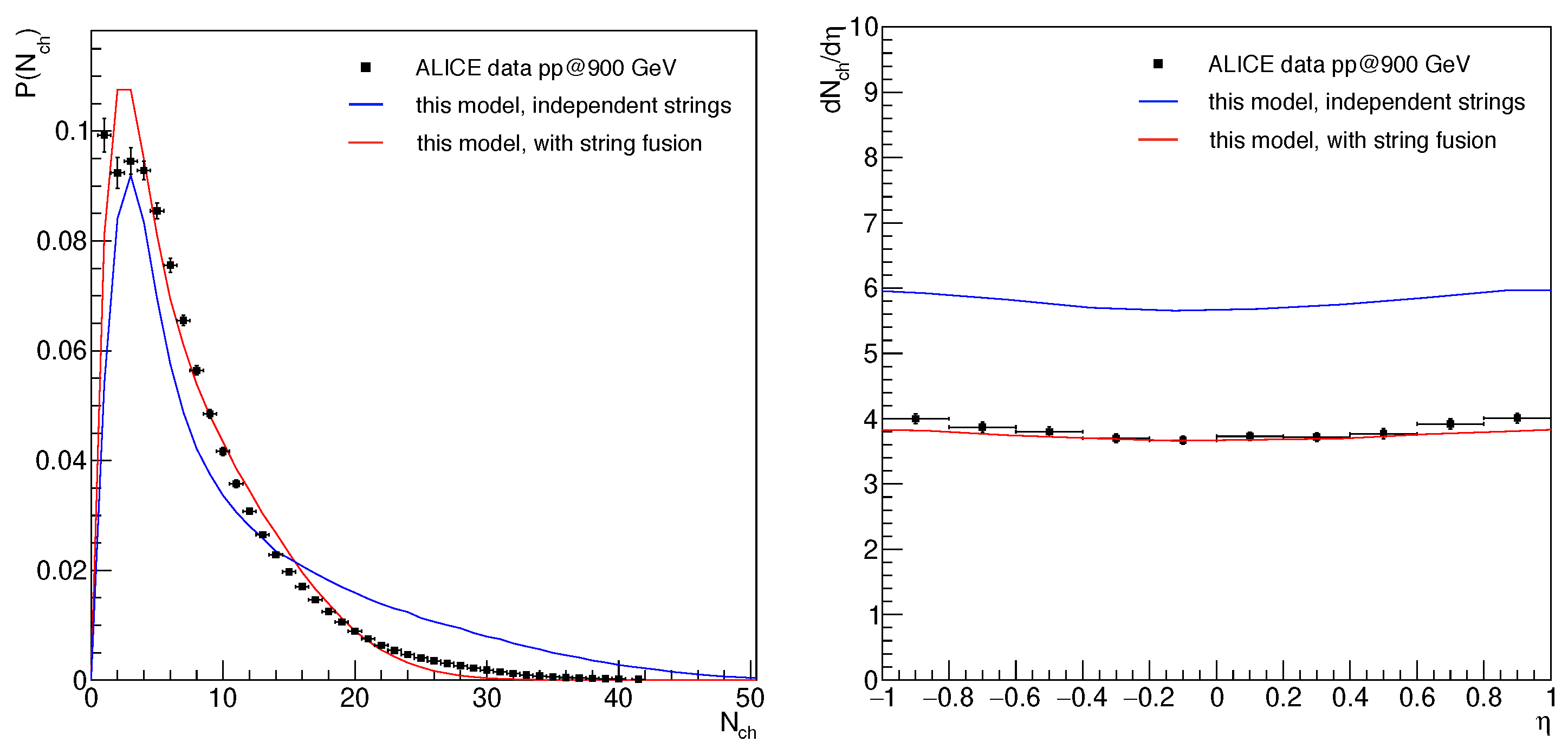
We tune our model with interacting particle production sources, evolving till
, to describe the ALICE data [
26] at midrapidity (
Figure 1). To describe the charged particle multiplicity distribution, the events with
are removed since these events are highly influenced by diffractive processes that are not considered in the model. For comparison, we also present here the results for the case of the absence of string interactions with the parameters obtained from the fit. One can see from the multiplicity distribution (
Figure 1, left) and pseudorapidity spectrum (
Figure 1, right) that the inclusion of the string fusion effect resulted into a relatively smaller average multiplicity.
One should keep in mind that, in the case of the multiplicity variable, the model can be retuned so that the no-interaction scenario would describe these spectra. One can see how important is the string fusion solely at the level of correlations, as described in the following Subsections.
Finally, it should be noted that
GeV/
c is selected in order to describe
GeV/
c measured by ALICE [
27].
3.2. –N Correlation Function
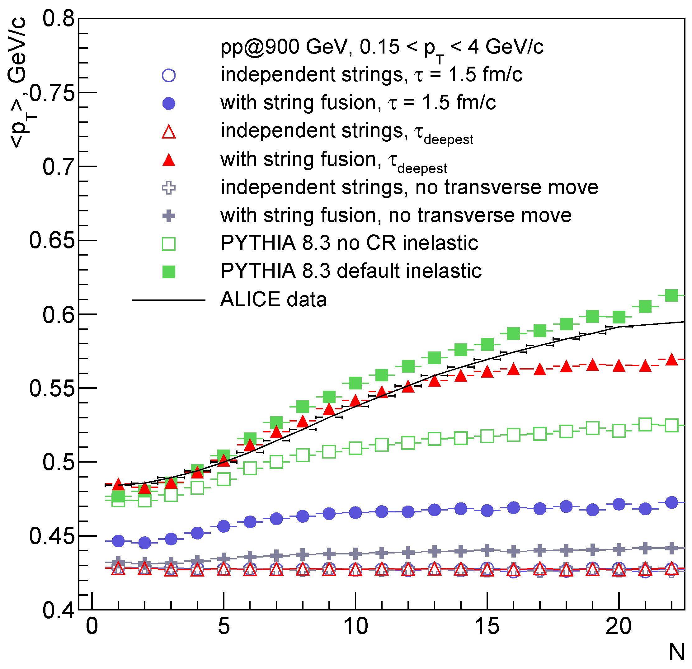
We study
–
N correlations in the acceptance of
GeV/
c,
. The model results with interacting particle production sources, evolving till
, tuned to the ALICE data [
27], are compared to the PYTHIA simulations and to the findings with other model options in
Figure 2.
From
Figure 2 one can see that the model results for independent strings (empty markers, except the squares) almost coincide, and they exhibit no dependence of
on
N regardless the transverse string dynamics. Thus, one can conclude that there is no collective behaviour without strings’ interaction.
As for the interacting particle production sources, one can see more significant correlations in
Figure 2 for the cases with the larger strings’ density formed in the event configuration. Namely, the first case is the weak
–
N dependence for string fusion and fixed strings’ positions in the transverse plane (full grey crosses): fusion occurres quite rarely. Next case is the correlation function for the system of strings evolving till
fm/
c (full blue circles). The largest
–
N correlation in the model is seen for the largest density of strings at
, where the string density is the highest one.
One could also see that the colour reconnection option in PYTHIA (full green squares) plays formally a similar role as our string fusion mechanism, although PYTHIA without the colour reconnection included (empty green squares) still has some background correlations.
In brief, even though one may try to tune global observables without collective effects of some sort, it is not possible to explain the growth of the event mean- with the multiplicity.
3.3. Multiplicity Correlations
Now, we study the multiplicity correlations in pseudorapidity in terms of the correlation coefficient,
, which represents the slope of the correlation function,
[
29],
defined for multiplicities
and
in two pseudorapidity intervals, (so-called “forward” and “backward”) separated by a
gap.
Correlation function,
, indicates how average value of
depends on the selected value of
. In case of a linear dependence the correlation coefficient reads [
30]:
It is important to mention that, in the case of a boost invariance in rapidity, i.e., when the string longitudinal dynamics is ignored, the fluctuations in the number of strings would provide the same input to the long-range correlations at all positions of forward and backward rapidity windows. This is not the case in our model, as with the loss of translational invariance, one might obtain different “volume” fluctuations (fluctuating number of strings acting as particle-emitting sources) for different .
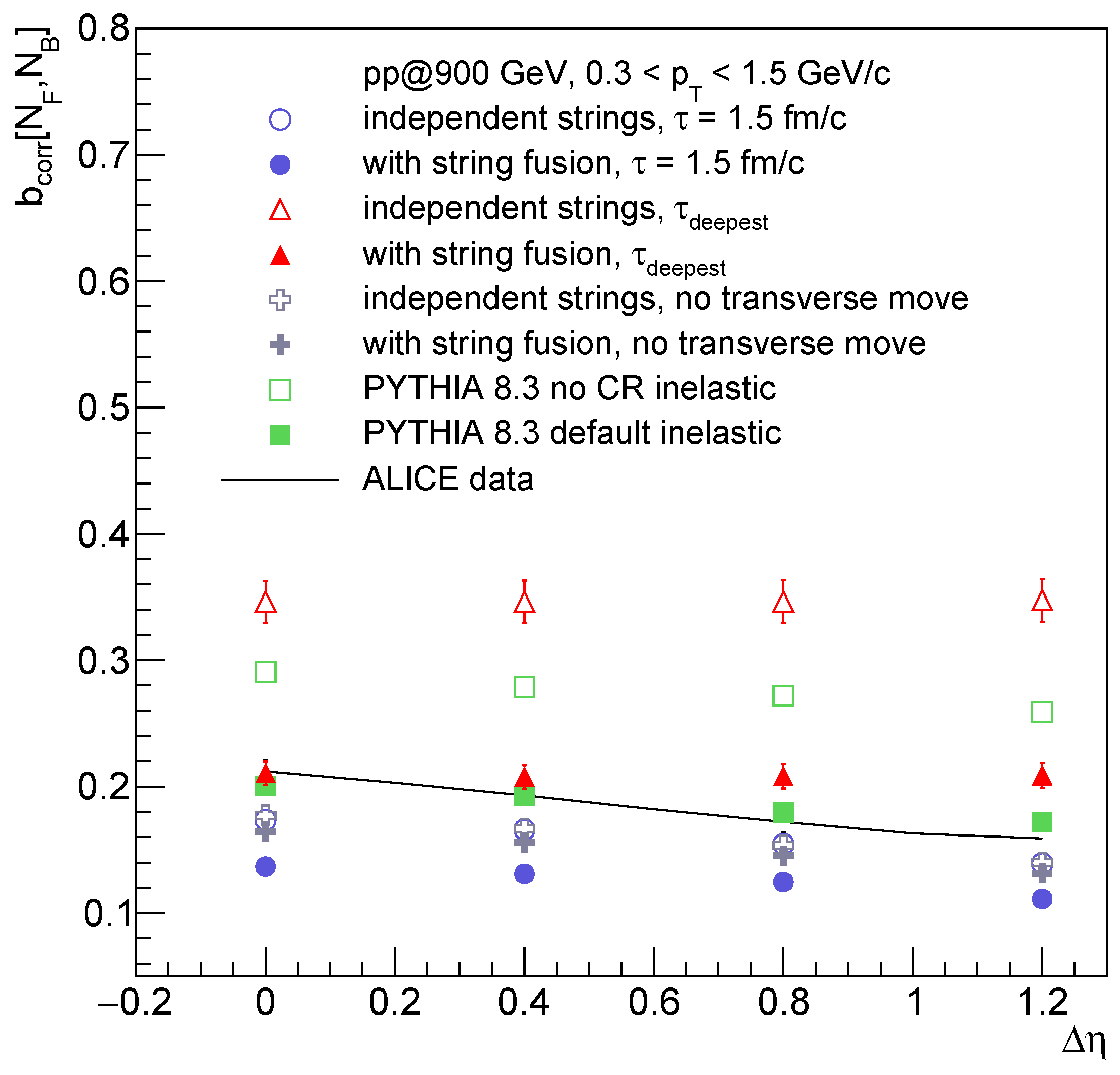
We study
as a function of the distance
between forward and backward pseudorapidity acceptances of width
each in order to access the information about particle sources and their distribution over
. As one can see from
Figure 3, the behaviour of
versus
is not trivial for a purely symmetric
-distribution, shown in
Figure 1, right.
Figure 3 shows two groups of results. The first is a set of plots for
versus
, which for
, exhibit almost no dependence on
—both with (full red triangles) and without (empty red triangles) string fusion. This is because
is not that large (the average
at
GeV is about 0.73) and, therefore, the colour strings stay long enough to produce particles into both forward and backward
-windows. This is why one sees a strong correlation which does not weaken with
. Note that the magnitudes of
are different for various model assumptions, and the calculations for
with string fusion are closer to the experimental values.
The second group shows the decreasing tendency of for all other model cases. The values of fall down with the increase of since the colour strings are significantly shrunk by with a fm/c evolution time. Therefore, the strings impact more independently in forward and backward windows the more the windows are separated. Thus, the forward–backward correlation weakens with . As a cross-check, one can notice that the results for fm/c and for the case without transverse string dynamics almost coincide for independent strings (open circles and crosses). This is because in these both cases, fm/c for the longitudinal dynamics.
For the interacting strings, the results for
fm/
c lie below the case without transverse string dynamics because of the higher frequency of string fusion and, consequently, lower multiplicity in the former case then in the latter one. This is also correct for any system evolution time: the results for interacting strings lie below the corresponding plots for independent strings because of the lower multiplicity caused by string fusion in the former case. The same prediction on the suppression of
due to string fusion was obtained earlier for strings that are infinite in rapidity [
32].
A similar behaviour one can observe for the PYTHIA simulations: colour reconnection gives an effect similar to that for the string fusion mechanism—an overall decrease of multiplicity and that of .
The model results are also compared with the ALICE measurements [
31]. The simultaneous fit to the experimental
and
distributions allows us to reproduce the experimental value of
only in the midrapidity (interacting strings evolving till
at
). However, for the moment, the model does not follow the steady decrease of the data
: the full red triangles versus the black line.
To conclude here, we note that the evolution time and the relevant string density are found playing the major role in the magnitude of long-range correlation coefficient and in its behaviour with the distance, , separating forward and backward pseudorapidity acceptance intervals.
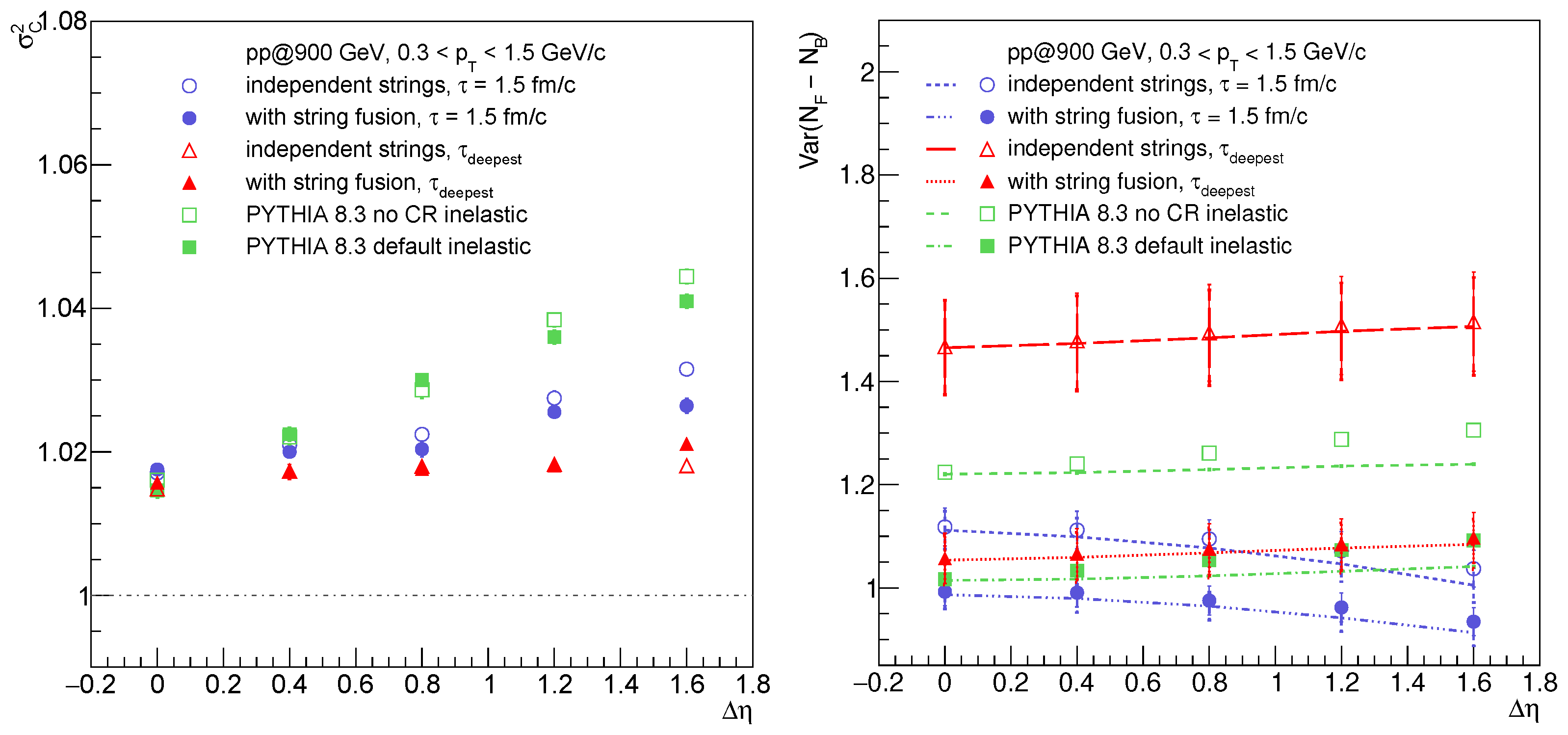
3.4. Multiplicity Fluctuations with Strongly Intensive Observable
To avoid the dependence of the results on the system “volume”, we study joint multiplicity fluctuations in forward and backward pseudorapidity intervals in terms of the special fluctuation measure,
[
33],
where
is a scaled variance of an extensive event variable
A distribution.
By construction, in the case of similar types of strings,
depends neither on the system “volume” (the number of particle-emitting sources), nor on its event-by-event fluctuations. As was proposed for the family of strongly intensive quantities [
34], the quantity
is normalised to unity in the case of the models of independent particle production.
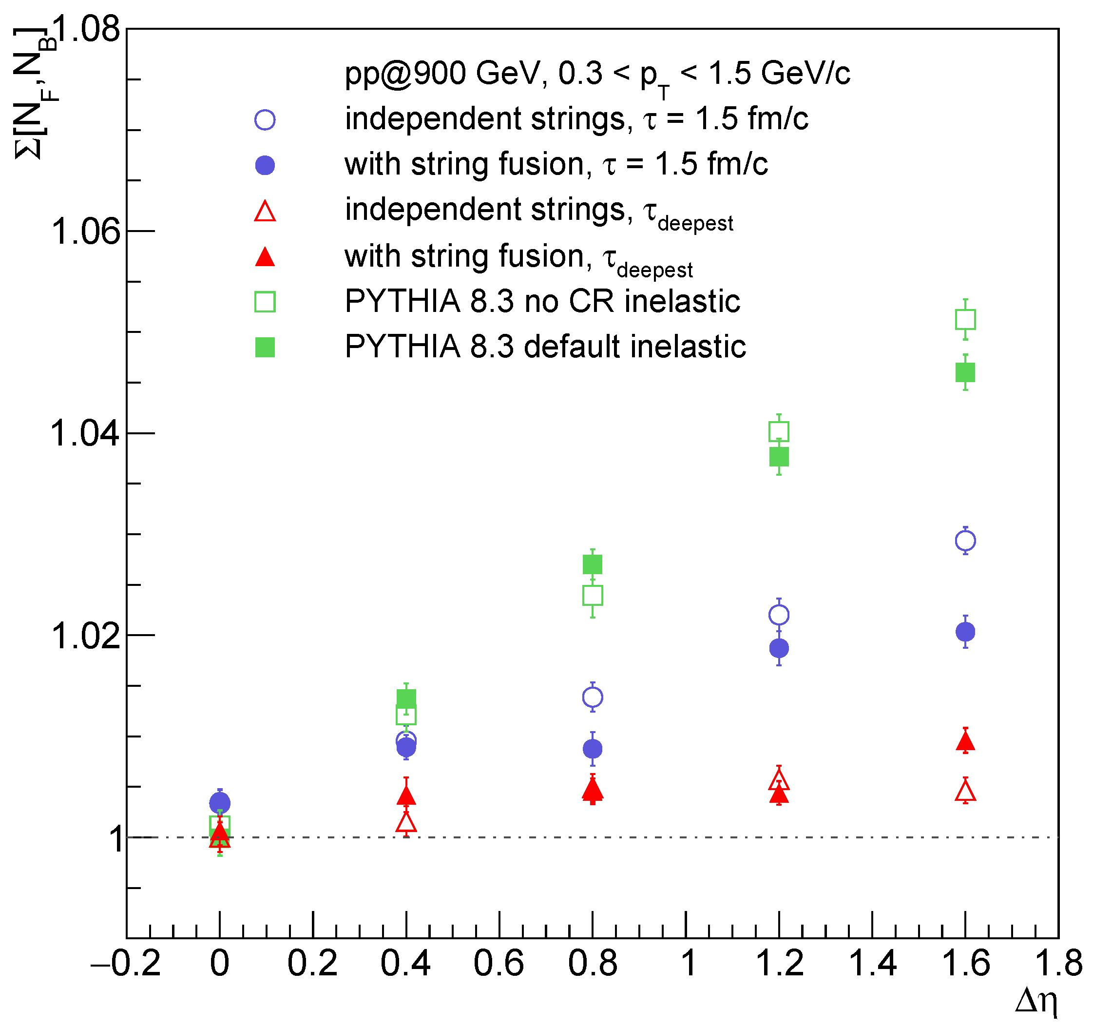
Figure 4 demonstrates an increase from the unity of
values with the distance between forward and backward
-acceptances. One can argue that the results for independent and interacting strings split, which made
dependent on the types of particle production sources. The results for
fm/
c (blue circles) tended to decrease for the case of string clusters for the largest
, which resembled also the difference for the PYTHIA plots (green squares). The results for
lied even lower (red triangles), although it is complicated to distinguish the two model regimes here.
A considerable difference with the PYTHIA predictions can be explained here by the absence of short-range effects in our model that was currently aimed at the study of long-range correlation effects.
3.5. Connection of with Cumulants and Factorial Cumulants
To illustrate the beauty of the mathematics standing behind the observable
, let us briefly discuss the
connection with the other often used objects, namely the cumulants and factorial cumulants. In the case of the joint probability distribution,
, the cumulants and factorial cumulants can be introduced for any linear combination of
and
. Following the notations of Ref. [
35], let us define a selected linear combination as a
q-vector,
. Let us consider these two specific
q-vectors:
and
, where
and
. The auxiliary
q-vectors that one needs in order to calculate cumulants and factorial cumulants are:
,
, and
.
Then, following Ref. [
35], one can immediately express the first-order and second-order cumulants for the joint probability distribution,
, in terms of the moments of the same distribution:
In turn, the factorial cumulants can be straightforwardly expressed in terms of the cumulants:
One could immediately notice the connection of the presented cumulants and factorial cumulants with the strongly intensive quantity in the case of symmetrical pseudorapidity intervals, i.e., when
:
This connection is not surprising as soon as the goal of the construction of these special observables (or ratios of observables) is to suppress trivial statistical fluctuations.
3.6. Connection of with
Asymmetry Coefficient
The main difference between the model results (
Figure 4) for
fm/
c and
comes from the geometry of the strings in an event (considering transverse dynamics, longitudinal loss, and cluster formation via string fusion). Indeed, as was already mentioned in
Section 3.3, the average
appears to be less than
fm/
c for this collision energy what results into different sets of strings and/or string clusters event-by-event producing particles in the forward and backward
-acceptances. Thus, another way to look at event-by-event multiplicity fluctuations is to construct an event observable,
that measures an event asymmetry in pseudorapidity [
36] and to study the variance,
, of its distribution over a set of events.
Let us consider the analytical form of
:
This observable has been extensively studied in different models [
37,
38,
39], e.g., in the cluster model of particle production, this observable helped to extract the average cluster size or, in other words, effective cluster multiplicity. Moreover, the extracted value both from pp and AuAu reactions was larger than the one predicted for the hadron-resonance gas model, indicating that correlations cannot be explained purely by the hadronic degrees of freedom considered in some statistical ensembles. In most of these studies, the two-stage scenario was adopted in one way or the other; some of the models take into account string interaction, while others provide a non-trivial non-uniform in rapidity fragmentation function of particle-emitting sources, but none of them consider simultaneously longitudinal dynamics and collectivity as we did in our model.
Let us show that
is closely related to the strongly intensive quantity,
. Using the assumptions,
for the first and the second term of
(
24), respectively, one arrives at
where the last equality holds under the assumption of
; “cov” stays for covariance. Thus,
The assumptions (
25) and (
26) are in accordance with the approximate calculations of Ref. [
39], where deviations of
and
from
and
are considered to be small enough.
An important remark concerning
needs to be made. Despite the demonstrated connection with
, strictly speaking,
is not a strongly intensive observable and may receive additional contributions coming from the “volume” fluctuations, as the latter are, in general, not cancelled out without the assumptions (
25) and (
26). Nevertheless,
is considered as an important quantity since it shows the magnitude of the fluctuations in terms of event asymmetry in the longitudinal dimension, i.e.,
indirectly provides us with some information about the initial state.
Figure 5, left, shows that the variance,
, taken from the distribution of the asymmetry coefficient
C (
23), indeed exhibits a behaviour similar to
(
Figure 4). Although both quantities gradually rise with
,
is not reaching the unity for the close
-acceptances (
). As seen, in this region, there are the largest fluctuations of
, and respectively, the assumption of small deviations of event-by-event multiplicities from their average values does not hold.
Figure 5, right, displays the values of
above unity in a more detailed way. For two quantities that follow the Poissonian distribution, their difference would follow the Skellam distribution. Therefore, typically, the Skellam function is considered as a baseline in the studies of net-charge fluctuations. In our case, the numerator of
can be treated as a net-hadronic charge in rapidity. The values of the model results of
, in
Figure 5, right, lie slightly above the corresponding Skellam baselines calculated as
. Therefore, the ratios of those model values over the lines are equal to
, which is slightly above the unity.
Following Ref. [
36], we may suggest that, at
= 0, strings and/or string clusters predominated, which produce particles in both forward and backward
-acceptances, which suppressed the value of
and
. With the growth of
, one expects more and more rare contributions of such sources. Instead, there were “short” quark–gluon strings that appeared only in the forward or in the backward
-intervals.
One has to mention that the same qualitative behaviour of
with
was obtained in Ref. [
40], where the authors considered only strings infinite in rapidity, but included the short-range correlations. Thus, one may argue that both the absence of short-range correlations and the presence of short strings in our model gave the same results for
that indicates the importance of the coherent application of the two approaches.
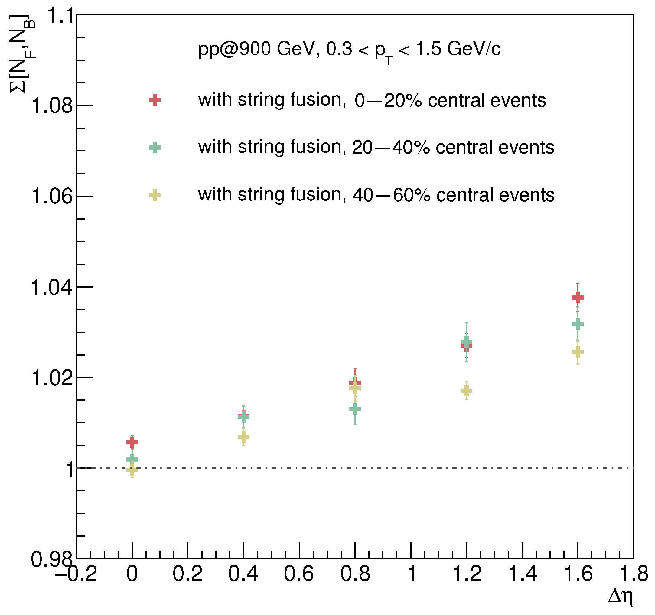
3.7. Forward Multiplicity Studies
In the analysis of the experimental data, along with the choice of stable variables, such as , another possibility to control an event’s initial conditions (such as unavoidable fluctuations due to, for instance, Fermi motion) is to select for analyses some sort of similar events.
In the context of the present study, it is necessary to make an important remark. We followed the picture of multi-pomeron exchange, which is needed to restore the unitarity of the scattering amplitudes for a pomeron intercept larger than one. Each cut pomeron resulted in the formation of two colour strings, which in total led to the formation of the number of strings in an event. In turn, each string had to be attached to either valence or sea quarks (at the moment, diquarks are not considered), which defines the number of partons “participating” in the interaction. Therefore, events differed by the number of participating partons, e.g., the number of colour strings that form the effective “volume” of the system radiating particles.
In this way, here, we repeat the procedure used in the ALICE experiment to define multiplicity-based classes of events in proton–proton collisions following Ref. [
41].
Knowing
for each particle, we plot the multiplicity of particles that fly in the V0-detector of ALICE [
42], whose acceptance covers
and
. This was to avoid auto-correlations in the TPC (Time-Projection Chamber) acceptance, where one measures particles for the analysis. We divide the distribution into five classes, each of which contained 20% of the events. For the analysis, the 0–20%, 20–40%, and 40–60% classes are taken and the corresponding strongly intensive quantity (
11) is calculated for each set of a specific class of events.
It is important to mention that the acceptance of the ALICE V0-detector covers the region where quasi-diffractive processes play a role. Furthermore in this region, it is crucial to properly model the string fragmentation close to the string endpoints, e.g., to take into account the possibility to have a diquark as an endpoint, which can produce additional baryon yields, etc. Finally, these detectors have non-ideal resolution, and hence, this factor has to be included in the simulations as well. All these effects are not taken into account in this version of the model. Because of this, we do not perform any direct comparison with the available experimental data [
41] obtained in very narrow multiplicity-based event classes. We only study whether
depends on an event “type” and whether the property of strong intensity is violated for
.
In
Figure 6, one can see that, for all multiplicity-based event classes,
(
11) exhibits the same trend of an increase with
. Moreover, one can see that, for more central events, this quantity reaches larger values. The same effect was observed by the ALICE experiment [
41]. This is another manifestation of the string fusion effect because, for more “central” events, i.e., events with the higher forward multiplicity, one has a larger number of cut pomerons and, consequently, a larger number of strings. This means that one has a higher probability of strings interaction and possibly could produce string clusters of higher string tension. A similar analysis with the same conclusion was performed recently in Ref. [
40] for interacting strings that are infinite in rapidity. Again, let us to emphasise the importance of taking into account both the short-range correlations that were modelled in Ref. [
40] and the initial conditions that are considered in this model, e.g., strings of short length and/or shift with respect to midrapidity, as these two effects give similar results and cannot be easily disentangled by analysing
only.
4. Discussion
Within the developed Monte Carlo multi-pomeron exchange model, we have obtained results on multiplicity and transverse momentum correlations for pp inelastic interactions at GeV. The key elements of the model based on the event-by-event formation and fusion of longitudinally extended colour strings are the long-range correlations naturally introduced. The correlations appear from the fluctuations in the number of “long” strings that produced particles simultaneously in the forward and backward pseudorapidity intervals.
Tuned to some global observables in the ALICE data, such as the rapidity distribution of charged particles for inelastic pp interactions at GeV and a –N correlation function, the model with string fusion and the evolution time gives results in qualitative agreement with the experiment in versus the distance between the forward and backward pseudorapidity acceptance intervals.
Strings’ evolution time and the relevant string densities are found to play a major role in the magnitude of long-range correlation coefficient and in its slope with the distance .
Results are found in trend with PYTHIA 8.3 event generator simulations, where the Colour Reconnection option plays a formally similar role, although the underlying physics of PYTHIA 8.3 is different.
Although it might seem, from
Figure 3, that our model contains also short-range correlations that are visible at small
in the
plots, we would like to stress that this is just a result of the modification of the long-range correlation background because of the appearance of short strings (with respect to forward and backward
-windows). Thus, in the present study, the short-range correlations have been effectively implemented in the model via the presence of short strings that independently impact the forward and backward pseudorapidity intervals.
A similar phenomenon has exhibited itself in the case of the application of the strongly intensive quantity
aimed at eliminating the trivial effects of the so-called volume fluctuations, as it drives
increase with
, which, in the case of the absence of longitudinal dynamics, may have originated only from the short-range correlations, as was shown in Ref. [
43]. In future, we plan to introduce genuine short-range correlations related to string hadronisation, resonance decays, or mini-jets and profit from their interplay with the string fusion mechanism.
The dependence of on the multiplicity-based event classes is found in accordance with the preliminary ALICE data: the model predicted larger values of for pp interactions with higher forward multiplicity.
We have also shown that is connected with such often used observables as cumulants, factorial cumulants, and the variance, , of the asymmetry coefficient distribution, which is also proven in the model simulation.
In this study, we have also shown that the introduction of the string fusion effect in the model results in the enhanced –N correlation as the fused strings, on average, decay to the smaller number of particles with higher s.


