Alfvén Wave Conversion and Reflection in the Solar Chromosphere and Transition Region


School of Mathematics, Monash University, Clayton, VIC 3800, Australia
Physics 2022, 4(3), 1050-1066; https://doi.org/10.3390/physics4030069
Submission received: 13 June 2022
/
Revised: 8 August 2022
/
Accepted: 25 August 2022
/
Published: 8 September 2022
(This article belongs to the Special Issue A Themed Issue in Honor of Professor Marcel Goossens on the Occasion of His 75th Birthday)
Abstract
:Series solutions are used to explore the mode conversion of slow, Alfvén and fast magnetohydrodynamic waves injected at the base of a two-isothermal-layer stratified atmosphere with a uniform magnetic field, crudely representing the solar chromosphere and corona with intervening discontinuous transition region. This sets a baseline for understanding the ubiquitous Alfvénic waves observed in the corona, which are implicated in coronal heating and solar wind acceleration. It is found that all three injected wave types can partially transmit as coronal Alfvén waves in varying proportions dependent on frequency, magnetic field inclination, wave orientation, and distance between the Alfvén/acoustic equipartition level and the transition region. However, net Alfvénic transmission is limited for plausible parameters, and additional magnetic field structuring may be required to provide sufficient wave energy flux.
1. Introduction
It is well-understood that magnetohydrodynamic (MHD) waves in continuously nonuniform plasmas exhibit ‘mixed properties’ [1], in that their natures—fast, Alfvén or slow—can differ in different regions of the domain. This is frequently discussed under the umbrella of ‘mode conversion’ [2], for example between fast and slow [3], fast and Alfvén [4], and slow and Alfvén [5]. It also includes the process of resonant absorption [6] most commonly discussed in the context of damping of oscillations in coronal loops, but which is just a particular manifestation of fast/Alfvén conversion followed by phase mixing and ultimate thermalization [7].
Mode conversion, or mixed properties, are important for several reasons. First, understanding them helps us interpret observations of the magnetic solar atmosphere. However, more importantly for the workings of the Sun itself, they provide avenues for mechanical wave energy to propagate from the photosphere, where it may have been generated by convective buffeting or have emerged from the Sun’s internal seismic waves, to the corona. Our star’s spectacular outer atmosphere, the corona (or ‘crown’), best seen at eclipse, reaches temperatures of over 1 MK, compared to the few thousand degrees of the photosphere, and is the seat of the solar wind that shapes Earth’s space environment.
There is good reason to believe that MHD waves observed in the quiet solar corona carry enough energy to heat it and to accelerate the wind [8,9], or at least to contribute substantially [10,11]. For the most part, these high energy-content waves are transverse in nature, driven largely by magnetic tension, leading to them being called ‘Alfvénic’ by some researchers. Others insist that they are more properly categorized as kink waves [12,13], though of course this requires the presence of cross-field structuring; flux tubes or flux slabs. Irrespective of this, the question arises, how do such waves reach the corona from the photosphere?
The epithets ‘fast’ and ‘slow’ refer to the local wave propagation speeds relative to the sound speed c and Alfvén speed a. Locally, a fast wave is faster than either of these, and a slow wave is slower than both. The Alfvén wave travels at the Alfvén speed, and hence is intermediate between the other two. In the simplistic layer-view of the quiet solar atmosphere (i.e., away from active regions or sunspots), the 6000–20,000 K chromosphere of around 2000 km thickness is topped by the precipitous Transition Region (TR) of only a few hundred km, across which the temperature rises to over 1 MK, and then the large-scale corona.
At its most basic, the chromosphere is a layer where the sound speed varies quite slowly (as the square root of the temperature), whilst the Alfvén speed increases exponentially with height (as the inverse square root of the density, approximately). There is some height therefore at which c and a coincide, which is called the equipartition height. This is where partial fast/slow conversion may occur [3], dependent on several factors including the attack angle between the wave vector and the magnetic field.
A few density scale heights above the level, where , the fast wave dispersion relation is approximately , where is the angular frequency and is the wave vector. Altitude corresponds to the coordinate z. With given fixed and , this implies wave reflection at , i.e., where the horizontal phase speed matches the Alfvén speed. This will normally occur somewhere in the mid to upper chromosphere, depending on frequency and how close to vertical the wave was launched. The slow wave in is essentially a field-guided sound wave, and is very prone to steepening and shocking [14], and therefore dumps the bulk of its energy there. So, just based on the fundamental properties of fast and slow waves and the strong stratification of the chromosphere, it would appear that these two wave types cannot supply the ubiquitous transverse waves observed in the corona.
Magnetic loops associated primarily with active regions can act as wave guides and support further wave types (slow and fast kink, sausage, etc., [15,16]), but the focus is on quiet Sun here. Spicules occupy less than 2% of the solar surface at any one time [17], and these are ignored too. The purpose here is to explore the options for transmitting transverse waves to the corona in an idealized horizontally homogeneous vertically stratified slab model only. As the fast and slow waves have already been dismissed, that leaves only the Alfvén wave. Or does it?
Although exciting Alfvén waves directly at the photosphere and having them propagate right through the chromosphere and transition region is plausible [18], there are issues with this idea, both as regards excitation and also the efficiency of penetration of the TR. Furthermore, strictly, in a uniform inclined magnetic field, to which attention is restricted, the only pure Alfvén wave mode must propagate in the vertical plane of the magnetic field and have its velocity polarization perpendicular to it. This is too restrictive, assuming waves at the photosphere will be launched with all orientations. In three dimensions, the mode types must couple.
Specifically, the various mode conversion processes discussed above, especially fast-to-Alfvén, present an opportunity for actually generating Alfvén waves in the upper chromosphere from fast waves before (or as) they reflect [4]. The efficacy of this is seen in the numerical experiments of Cally and Goossens [2].
The purpose of this contribution is to further explore the ability of the three basic MHD wave types to penetrate a vertically stratified chromosphere and TR to reach the corona, without the assistance of transverse structuring (flux tubes) that support their own range of leaky and non-leaky tube waves [19,20,21]. We are therefore extending the numerical analysis of Cally and Goossens [2] with the aid of recently developed exact three-dimensional (3D) series and asymptotic solutions [5] in a two-isothermal-layer (chromosphere/corona) model with uniform inclined magnetic field. The new complete asymptotic solutions in particular improve our ability to model the injection of pure fast, Alfvén, and particularly slow waves at the base. We wish to determine what types of non-tube waves can best reach the corona, having fought their way through the highly stratified chromosphere and the even sharper transition region. This makes clearer the conditions under which substantial energy is transported, and provides a baseline for wave penetration to the corona.
Of course, the introduction of cross-field magnetic structuring such as flux tubes into the model opens up further mode types such as field-guided fast waves that may efficiently convert to Alfvén waves on resonant surfaces in the tubes as they bounce back-and-forth within slow Alfvén speed tubes, as discussed in detail in Cally [22]. This is the process of resonant absorption. Many authors find such magnetic structuring assists the propagation of Alfvén or Alfvénic waves to the corona (e.g., [22,23]). Further structuring such as neutral points and quasi-separatrix layers also afford opportunities for enhanced mode conversion [24,25], and clearly play important roles, including in the corona itself. Torsional Alfvén waves in flux tubes are also found to be adept at penetrating the TR [26]. These magnetic structuring effects are not considered here. Instead we focus purely on vertical gravitational stratification alone to determine the extent to which this first-order effect can provide sufficient Alfvén flux, and by implication the extent to which more complex structuring is required.
2. Materials and Methods
We explore a very idealized two isothermal layer atmosphere, representing the chromosphere at the bottom and the corona above. The thin transition region between them is represented as a discontinuity, as typically it is much thinner than the wavelengths at issue. The very basic nature of the model is designed to allow us to focus on the most fundamental issues of wave propagation and conversion in a strongly stratified atmosphere such as the solar chromosphere/TR/corona, and also allows us to make use of recently developed exact solutions. we assume ideal linearized MHD, ignoring such important physics as partial ionization [27,28] and shocks, both of which can contribute to mode coupling [25,29,30,31,32].
Exact two-dimensional (2D) solutions in an isothermal stratified atmosphere have long been known in terms of Meijer G-functions [33] or simpler generalized hypergeometric functions [34]. Zhugzhda and Dzhalilov [33] also sketched out the (convergent) Frobenius series solutions about and the leading order asymptotic solutions as for the 3D case, but did not couple the two. Recently, Cally [5] derived the complete asymptotic solutions as and numerically coupled them with the Frobenius solutions, allowing net mode conversion between fast, slow and Alfvén at the bottom (as characterized by the asymptotic solutions) and fast, slow and Alfvén at the top (the Frobenius solutions).
In this paper, we extend this analysis to the two layer model by using the exact solutions in each of the two layers, coupled at the TR discontinuity by the appropriate matching condition, that the plasma displacement and its first z-derivative be continuous (Section 2 in [35]).
2.1. Exact 3D Solutions in an Isothermal Atmosphere
We briefly summarize the Frobenius solutions [2] and complete asymptotic solutions [5] in an isothermal atmosphere.
The governing equations are best described in dimensionless form. Consider an isothermal atmosphere with uniform magnetic field
inclined at angle from the vertical and oriented angle out of the x-z plane. The density scale height is , where is the ratio of specific heats (taken as here) and g is the gravitational acceleration. we then introduce the dimensionless frequency and horizontal wavenumber . Without loss of generality, the wave has been oriented in the x-z plane, so .
Rather than altitude z, the dimensionless position is adopted, which increases downward from zero at . For convenience, , or , has been chosen to coincide with the equipartition level . The acoustic cutoff frequency is in these units.
Let the plasma displacement be , and introduce the dependent 6-vector , where the primes denote the derivative with respect to s. The sixth order matrix ordinary differential equation
governs the linearized oscillations, where is a matrix quadratic function of s. This admits convergent Frobenius series solutions
where the indices are the eigenvalues of ,
corresponding, respectively, to the growing and evanescent fast modes, the outgoing and incoming slow modes (if ; otherwise growing and evanescent), and the Alfvén mode (which has a double root).
The repeated Alfvén eigenvalue has geometric multiplicity 1, so Equation (3) only provides the first five solutions. The sixth, the second Alfvén solution, contains a logarithmic term,
Recurrence relations for the coefficients and are described in Appendix B of Cally [5]. These series all have infinite radius of convergence.
Conversely, the solutions in the neighbourhood of the irregular singular point () are only accessible asymptotically (Appendix C in [5]). Briefly,
- Fast waves: for the fast waves,where and is chosen from the nullspace of ,andSubsequent coefficients are determined from recurrence relations.
- Alfvén and slow waves: both the Alfvén and slow waves behave asymptotically asandHereSubsequent coefficients are again constructed by recursion.
The six solutions again correspond to the upward and downward propagating fast, slow and Alfvén waves, this time in a high-beta plasma (the plasma is the ratio of gas to magnetic pressure). However, the connection between the six top and six bottom solutions is not trivial, and is only accessible numerically by matching at an intermediate point at which the asymptotic series are sufficiently accurate but where the Frobenius series can still be evaluated with precision. (In the 2D case, the connections are known analytically). In practice, works well, but this sometimes needs to be adjusted.
2.2. The Two-Layer Model
The two layer model is characterized by the following parameters.
- Height of the TR discontinuity above the equipartition level in units of the chromospheric scale height;
- Temperature jump factor across the TR;
- Magnetic field inclination ;
- Wave orientation relative to the vertical plane of ;
- Wave type—slow, Alfvén or fast—injected with unit flux from ;
- Dimensionless frequency ;
- Dimensionless horizontal wavenumber .
Consequently, and jump by factor across the TR; scale height H jumps by the same factor; and s jumps by factor . Although and must be continuous across the TR, is discontinuous. Hence, the first three components of are continuous whilst the last three jump by factor . The primary output in each case is
- The upward Alfvén wave flux at the top ;
- The upward slow (acoustic) wave flux at the top.
Exact Frobenius and high-accuracy complete asymptotic solutions can be matched at a selected point in the chromosphere. Assuming the injected fast, slow or Alfvén wave at carries unit vertical wave-energy flux, one may then calculate the slow and Alfvén wave fluxes at the top in the corona. The fast wave is evanescent there, and so carries no flux. Results for a range of parameters are presented in Section 3.
The novel aspect of this work, relative to the single-layer exploration of Cally [5], is the two layers, so we are primarily focused on the effect of the transition region in reflecting and otherwise modifying waves that reach from their injection at as pure fast, slow or Alfvén. In particular, how are Alfvén waves in the corona best produced?
3. Results
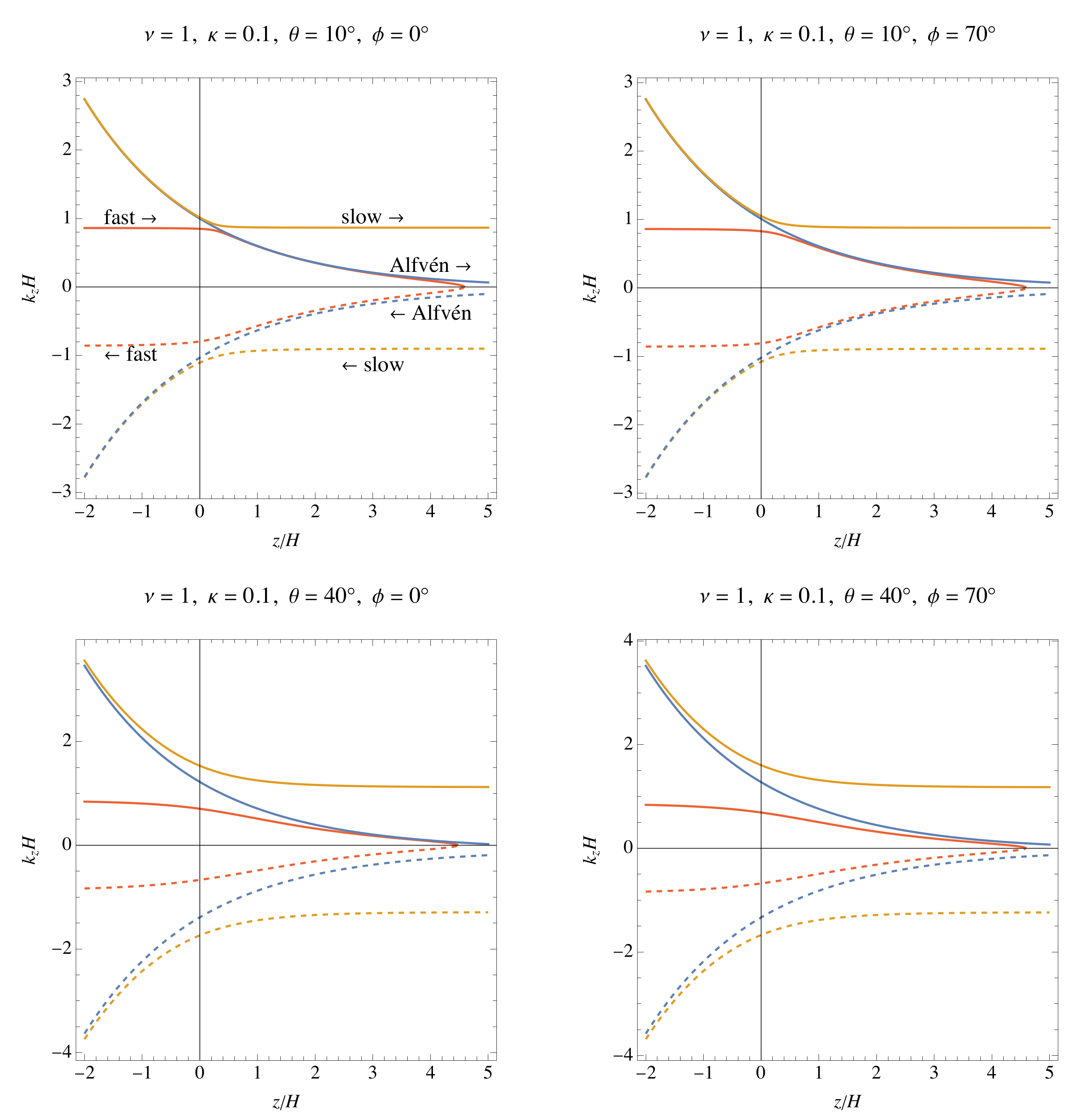
Dispersion diagrams in z- space illustrate how and where mode conversion of various types can occur in a stratified atmosphere. With frequency and horizontal wavenumber set and fixed, the dispersion relation (Equation (3) of [5]) represents an implicit link between altitude z and vertical wavenumber . This is plotted for an isothermal atmosphere in Figure 1 for the case , and and , with and . Upward propagating fast, Alfvén and slow loci are plotted as full curves, and downgoing loci as dashed curves.
It is seen that with there is a close avoided crossing between upgoing fast and slow waves in the top left panel (the 2D case ). This is where efficient fast/slow transmission occurs: fast-to-slow is acoustic-to-acoustic and is called transmission, and similarly slow-to-fast is magnetic-to-magnetic transmission. Fast-to-fast (acoustic-to-magnetic) and slow-to-slow (magnetic-to-acoustic) are both conversion, as the waves’ fundamental natures change. The gap between the downgoing fast and slow loci is noticeably wider, and so transmission is much reduced on this leg [3]. The upward avoided crossing is also wider and weaker when , as the attack angle between wave vector and magnetic field is larger.
We also notice a long near-degeneracy between the upgoing fast and Alfvén waves over , affording an opportunity for conversion between these two wave types. However, despite this opportunity, there is no such conversion in the 2D case , as the polarizations are orthogonal. In 3D though, such conversion can be very powerful [4].
Similarly, there is a near degeneracy between slow and Alfvén waves over that again allows conversion in the 3D case.
At much larger magnetic field inclination (bottom row), the fast/slow avoided crossing gap widens, and that conversion mechanism is weakened. The long near-coincidence of the fast and Alfvén branches is also shortened and weakened. Some slow/Alfvén conversion remains, as seen later, but it is not as strong.
3.1. Single Layer
For comparison with later two-layer calculations, we first look at weakly and strongly inclined magnetic field cases without transition region.
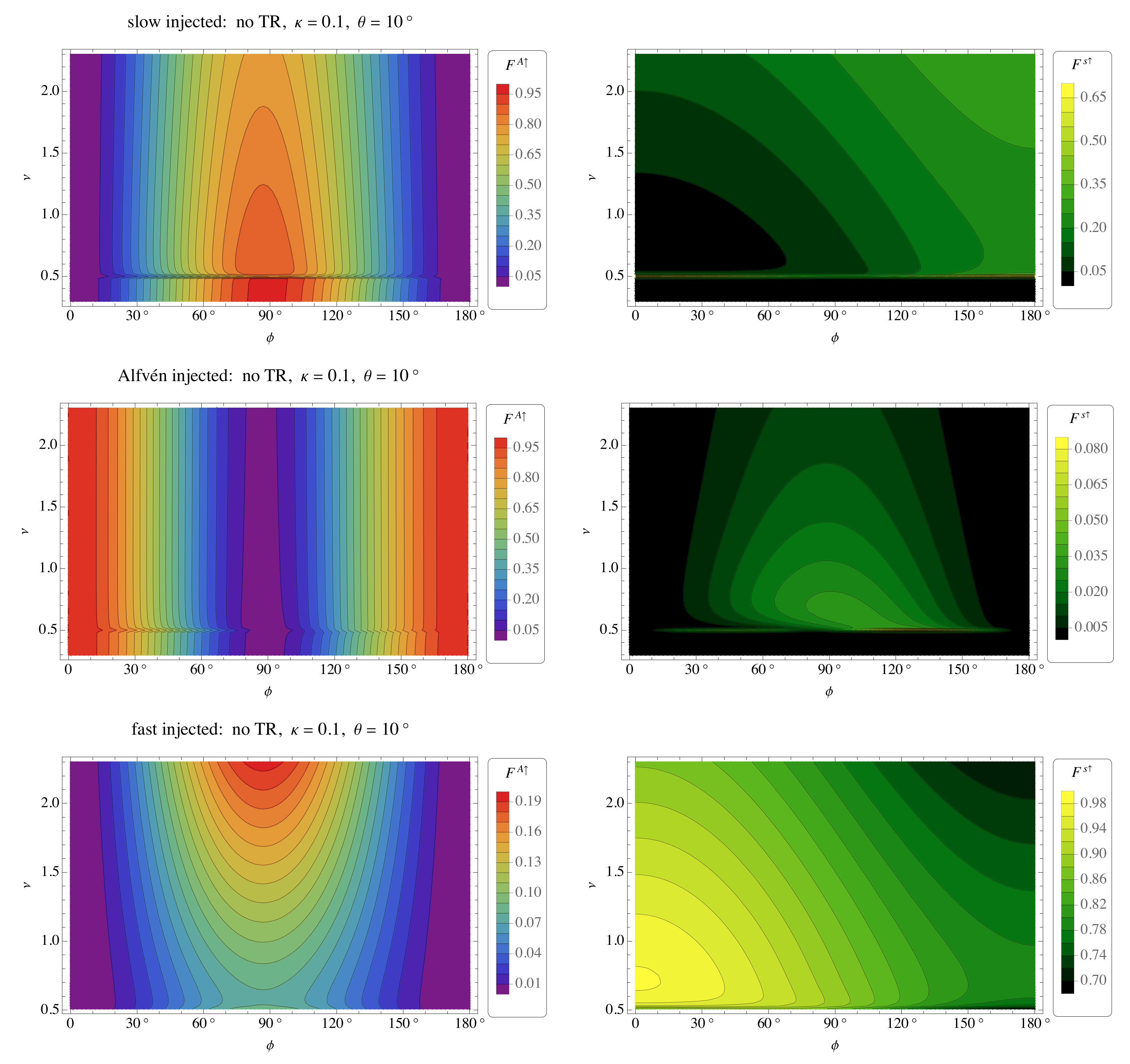
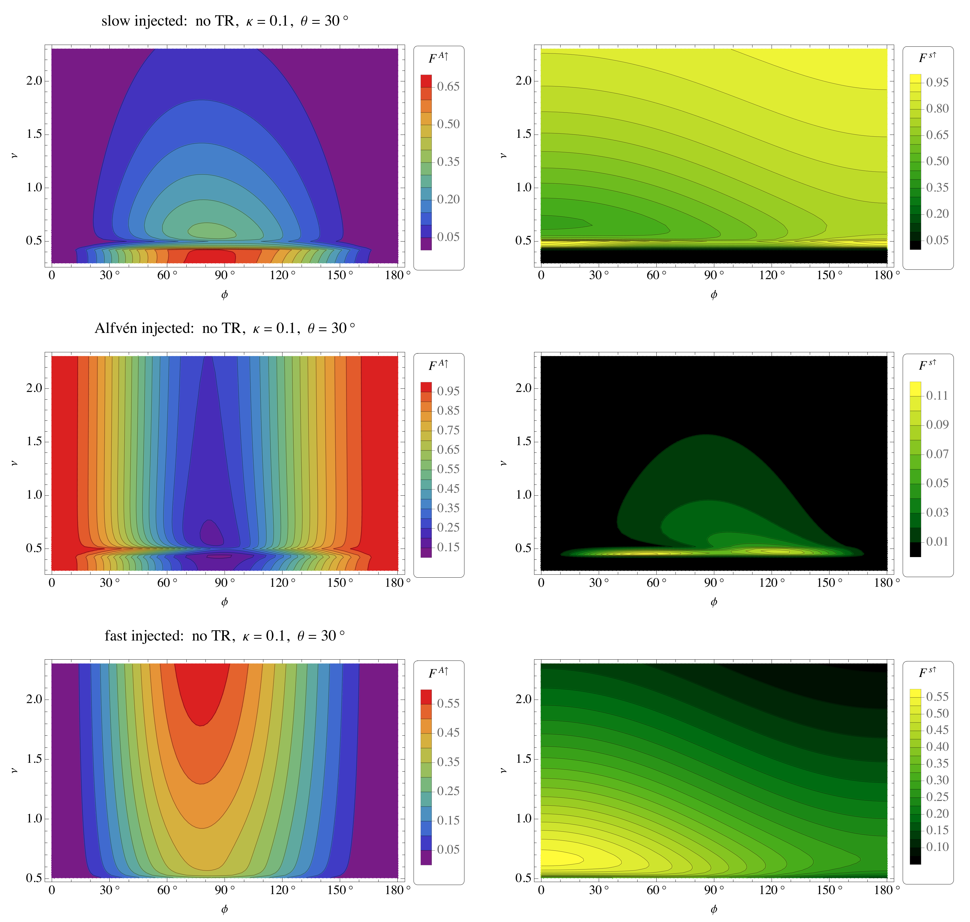
In Figure 2, with and , waves of frequency and unit flux are injected from () into an isothermal atmosphere with the magnetic field oriented at angle . The three types of injected wave are slow (top row), Alfvén (middle row), and fast (bottom row). The contour plots display the resultant top upward Alfvén (left column) and slow (right column) fluxes as functions of and . These fluxes sum to less than 1 as there is also some reflection and conversion to downgoing waves. The effect of the acoustic cutoff at is apparent. Slow and Alfvén waves are injected over , but the fast wave, which is essentially acoustic in the high-beta region, does not propagate there until , and hence only these higher frequencies are included in the bottom row.
On the other hand, the ramp effect allows acoustic waves to propagate vertically in a low-beta plasma if [3,36,37], i.e., , which is especially apparent in the right column for the case (Figure 3).
- In the top row, an injected high-beta slow wave is magnetic in nature and polarized transverse to the magnetic field, though orthogonal to the Alfvén wave in that region. Nevertheless, via several processes in the intervening layers, it emerges at the top as a mixture of Alfvén and acoustic (slow in the low-beta region). Near total conversion to Alfvén occurs below the acoustic cutoff frequency and at , and it remains strong at that orientation at higher frequencies too.
- In the middle row, the injected Alfvén wave largely maintains its identity throughout if is small, but slightly (a few percent) converts to upgoing acoustic waves via coupling. Mostly though, it reflects when is not small.
- In the bottom row, the injected fast (acoustic) wave couples significantly (up to 20% for and 60% for ) to the upgoing Alfvén wave, especially at and higher frequencies. It also partly transmits throughout as an acoustic wave, especially for small and .
Bear in mind though that these calculations are linear. In reality, acoustic waves in particular are susceptible to shocking and subsequent dissipation.
3.2. Double Layer
With many parameters defining the two-layer chromosphere-corona problem, we concentrate on surveying the top upward Alfvén and slow wave energy fluxes as functions of magnetic field orientation angle and dimensionless frequency for selected values of , , and , and also as functions of and for fixed , , and .
Recalling that is the acoustic cutoff frequency, typically around 5 mHz in the chromosphere, we restrict attention to , covering a physically interesting range of about 3 mHz to 23 mHz.
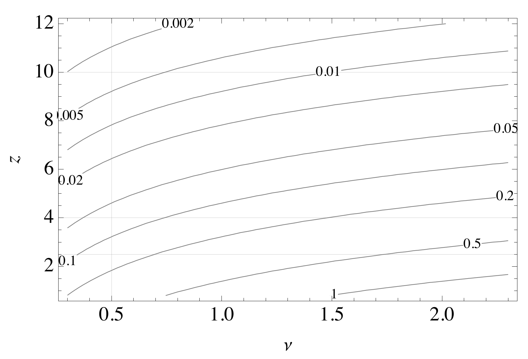
We next need to estimate the height of the fast wave turning point. As discussed earlier, this occurs about where , or in dimensionless terms where z is measured in units of the density scale height. Figure 4 plots contours in -z space. This allows determination of whether the fast wave impacts the TR, or how close it gets, for a given . For example, with , the fast wave does not reach a TR at over the plotted frequency range. The range corresponds to large scale waves, and is of most interest here.
The parameter represents the distance between the equipartition level and the TR, and is in effect a measure of the magnetic field strength. The stronger the magnetic field, the lower is the height of and hence the greater is . For example, in a sunspot umbra, typically lies a few hundred kilometres below the photosphere, whereas in quiet Sun it is generally in the low chromosphere, and can be identified loosely with the canopy. As the quiet Sun TR may be around 15 scale heights above the photosphere, we select and 10 to represent small and large gaps, respectively.
3.2.1. ,
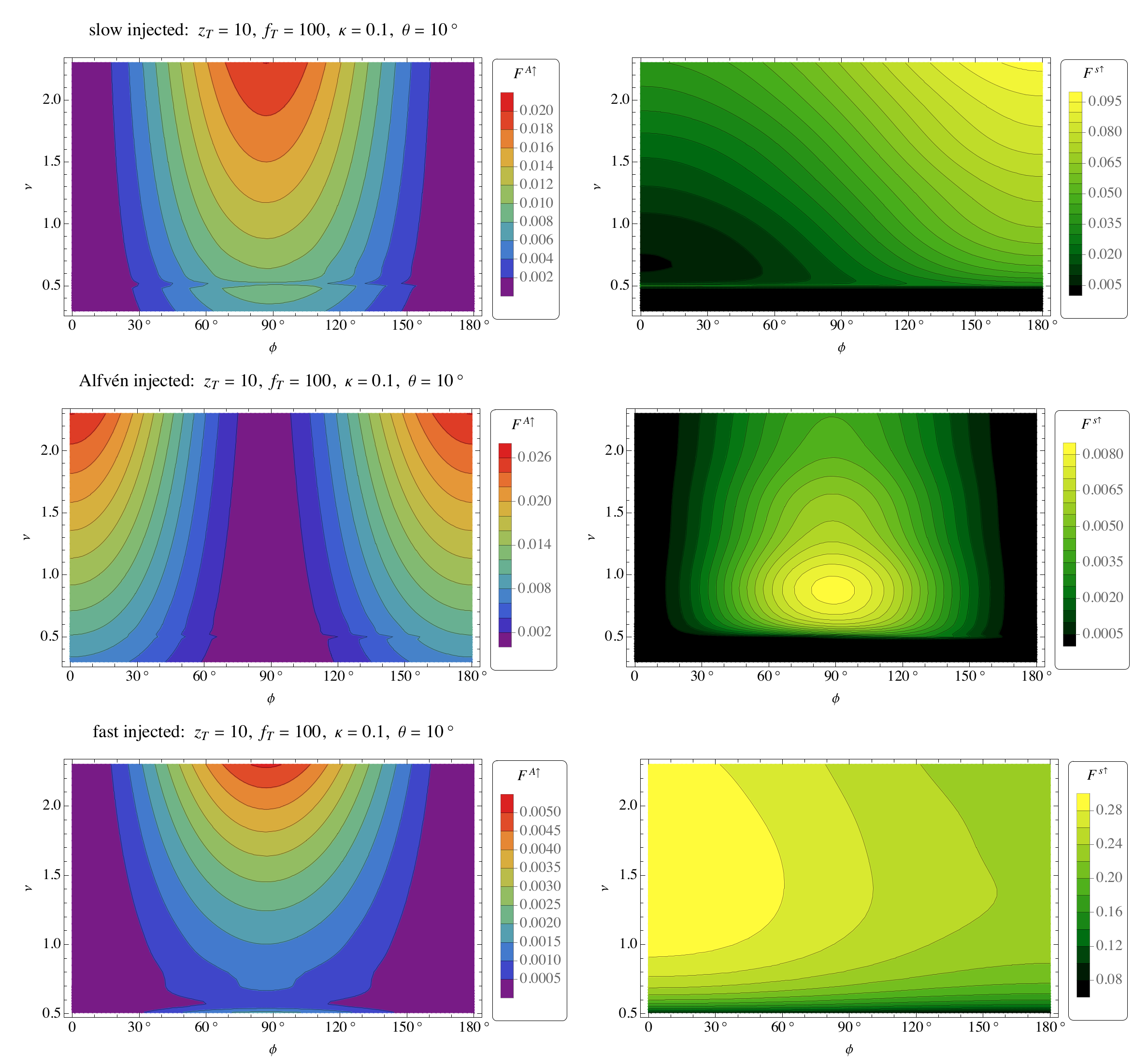
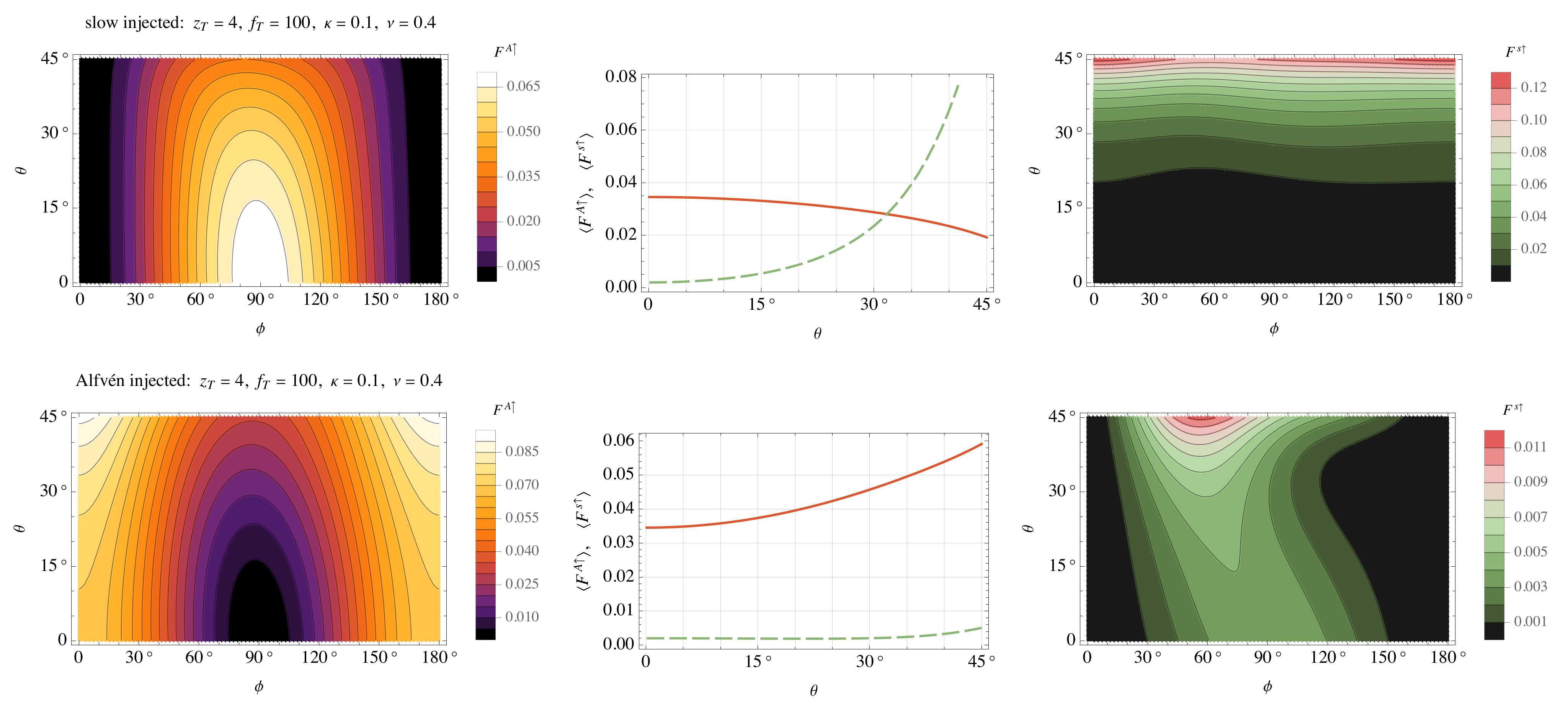
Now let us introduce a discontinuous transition region, and see what changes. In Figure 5, with and , a TR is introduced at and with temperature contrast , corresponding to a TR well above and a jump from 10,000 K to 1 MK for example. Unsurprisingly, this large sharp increase in temperature, and corresponding decrease in density, is highly reflective, especially for the Alfvén flux.
With these parameters, Alfvén fluxes of up to about 2% are obtained at high frequencies, both in the direct Alfvén-to-Alfvén case for small and via the slow-to-Alfvén route for . A smaller quantity for fast-to-Alfvén conversion is also seen at high . Slow-to-slow transport, especially at low , is by far the dominant transport mechanism, assuming no non-linear losses.
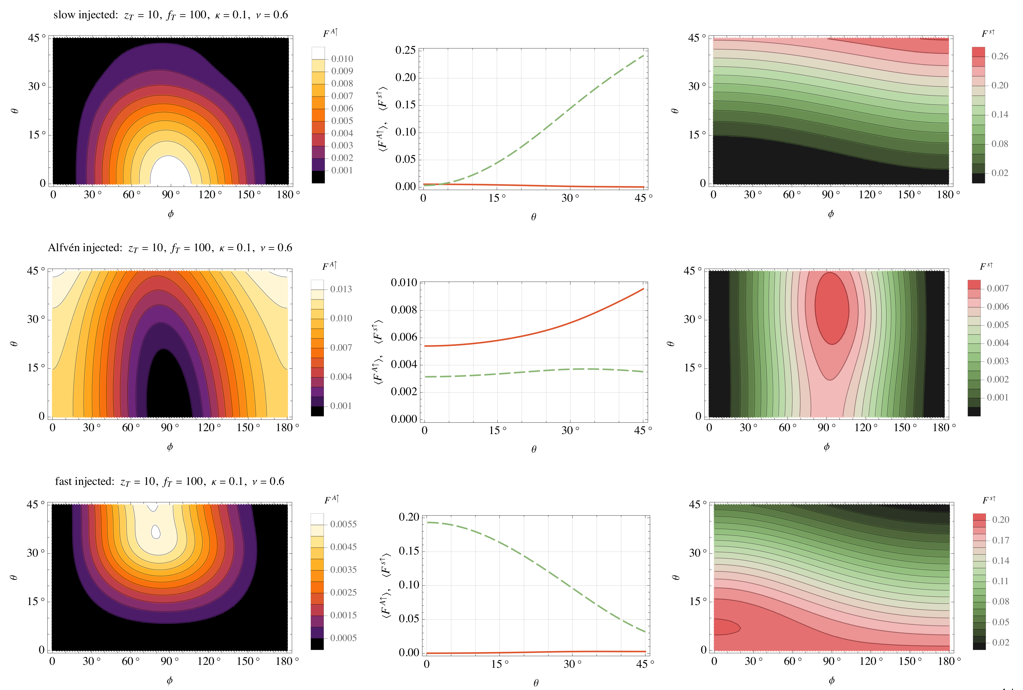
Figure 6 plots the same quantities over and for fixed and (slightly above the acoustic cutoff), and their averages over all orientations . The average over is of significance because the orientation of the horizontal component of the wavevector might be expected to be random. It is seen that the direct Alfvén-to-Alfvén route is strongest in the near-2D case of small and for highly inclined magnetic field, whereas the slow-to-Alfvén connection is most prominent for small inclination and . Net Alfvén flux does not exceed about 1% in this highly reflective scenario, though slow-to-slow and fast-to-slow transport can reach 20% or more.
3.2.2. ,
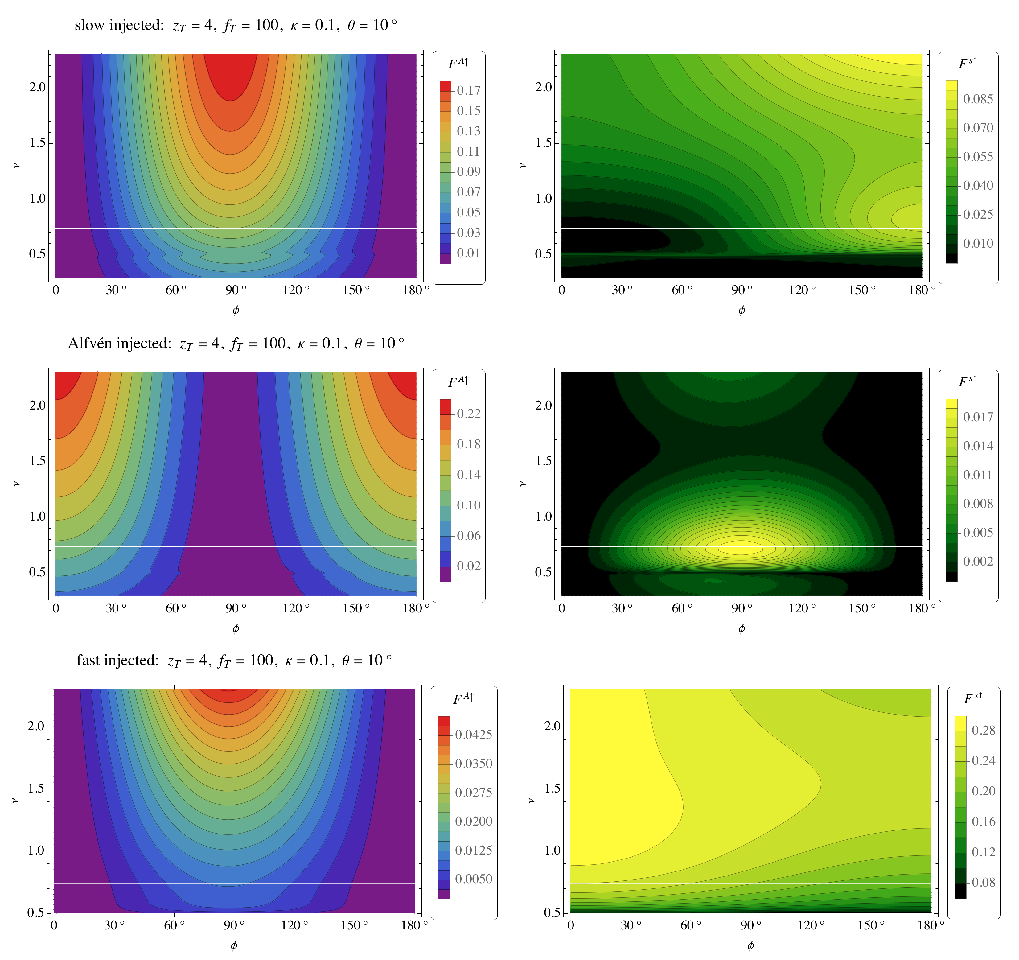
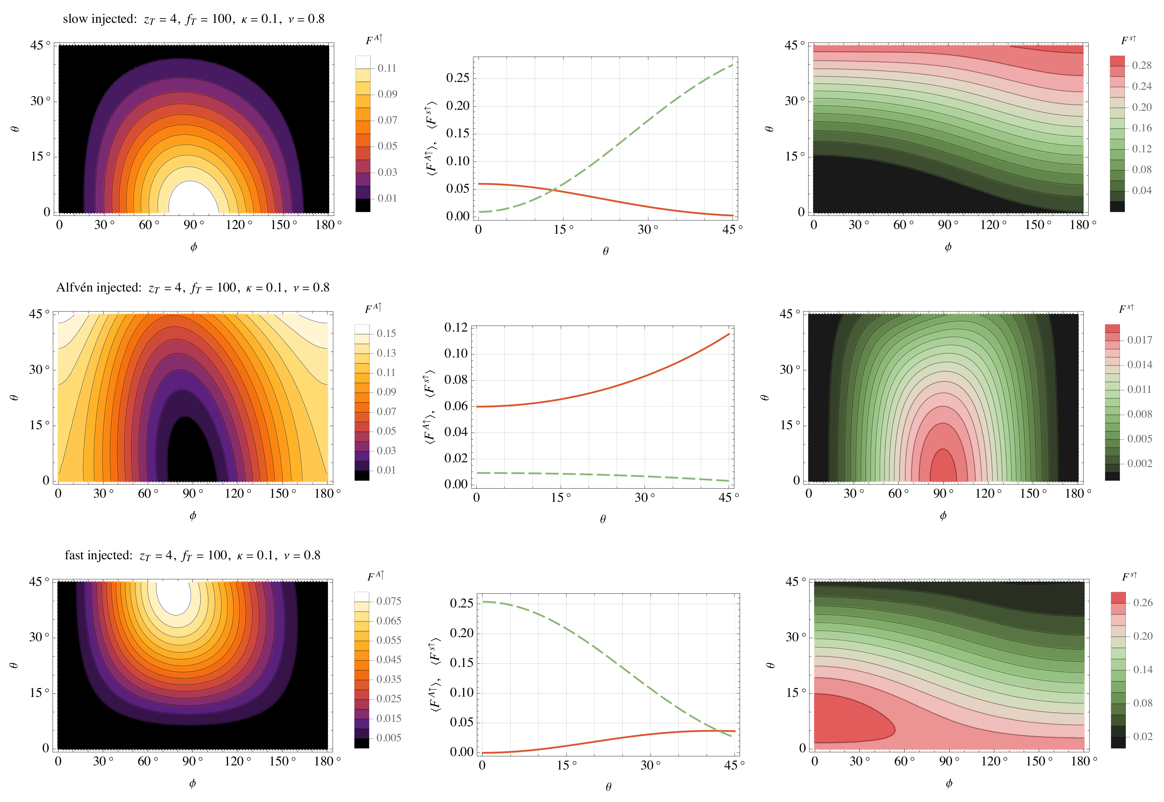
In Figure 8, the gap between the equipartition height and the TR is reduced to . This results in a much-enhanced coronal Alfvén wave flux at frequencies well above for , for which the fast wave reaches the TR before reflecting. Interestingly, this is more pronounced for the injected slow and Alfvén waves than for the injected fast wave due to strong mode coupling.
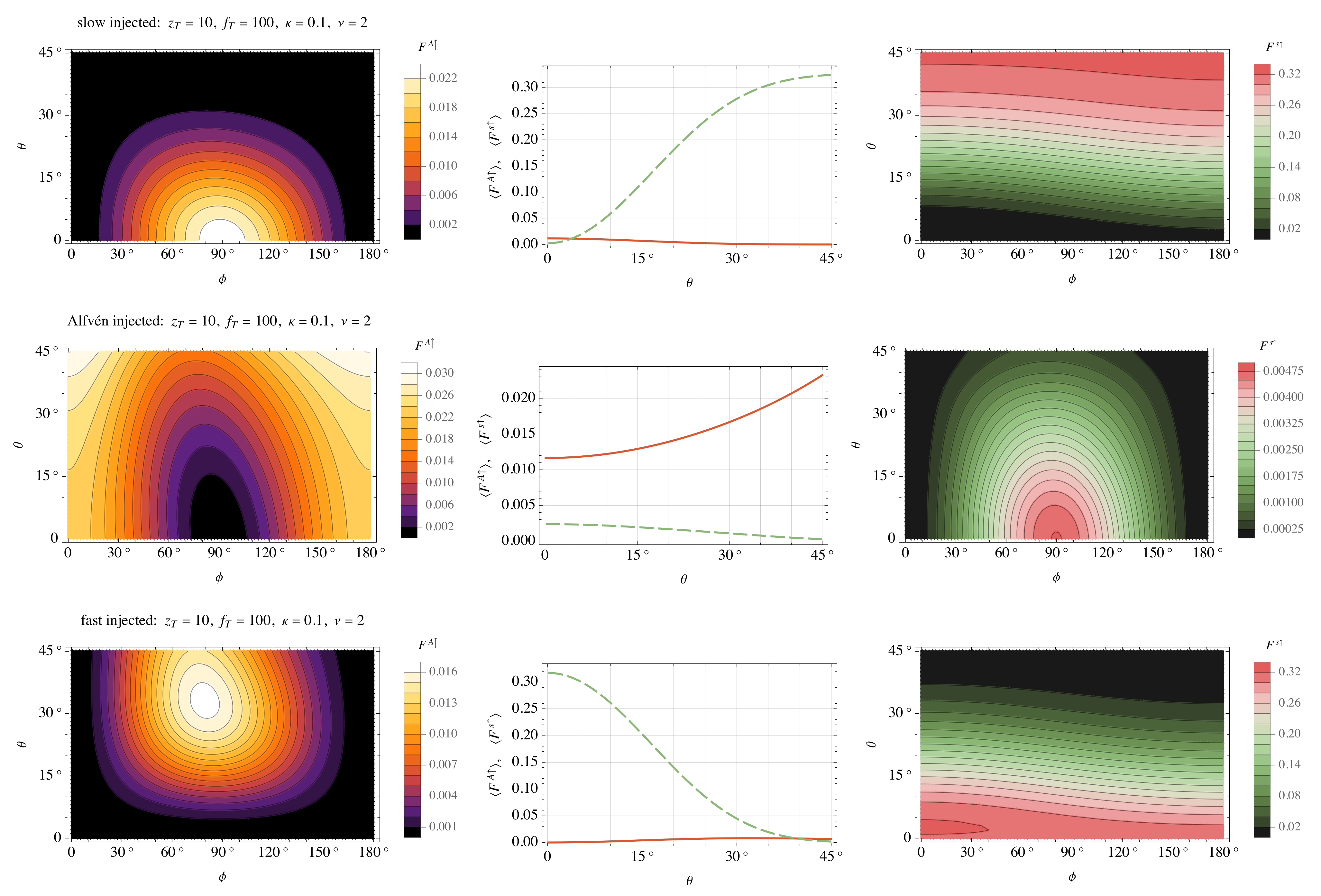
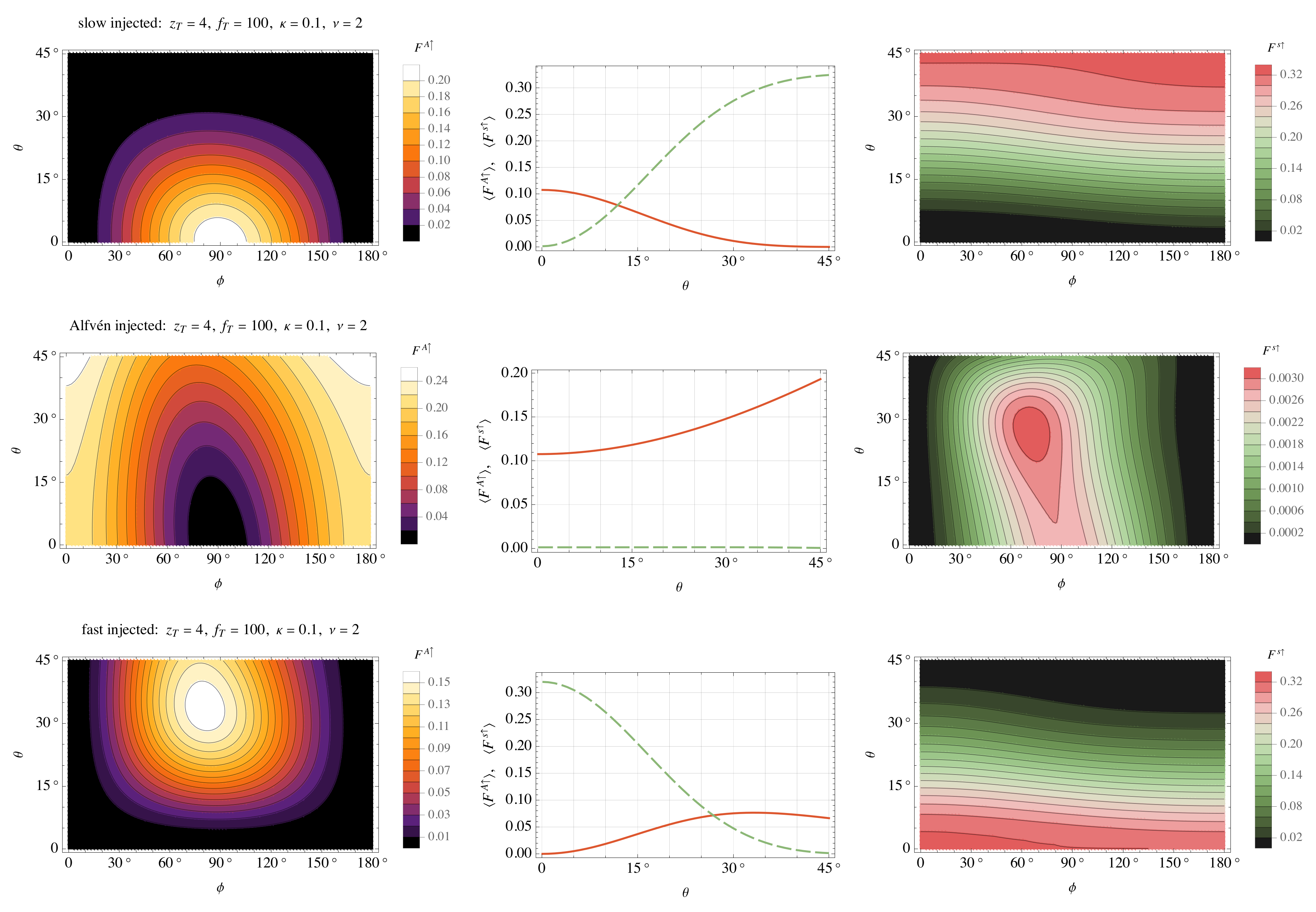
Figure 9, Figure 10 and Figure 11, for, respectively, , 0.8 and 2, again display the top fluxes as functions of and and as functions of when averaged over all . Alfvén fluxes are significantly enhanced in all cases, though slow-to-Alfvén is most pronounced at small inclination and ; Alfvén-to-Alfvén dominates at large inclination and small; and fast-to-Alfvén is strongest (a few percent) at to and .
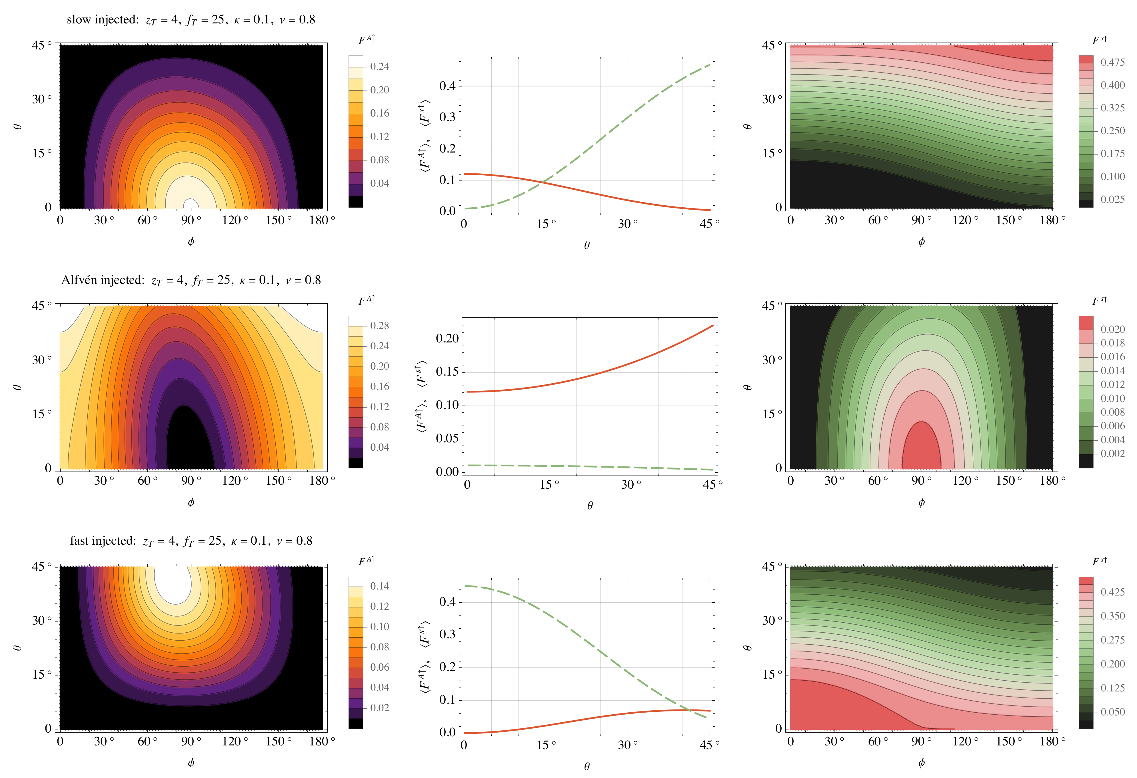
Finally, Figure 12 is again for the frequency , but with a much lower contrast transition region, . This is to allow us to estimate the significance of TR reflection in comparison to the of Figure 10. Broadly, it is seen that the top Alfvén flux is roughly doubled, suggesting that the Alfvén flux depends on approximately as . This is consistent with the classic transmission coefficient on a two-piece string with wave propagating from a region of wave speed to one with faster speed : ∼ for , where .
4. Discussion
This article has explored how injected slow, Alfvén and fast waves from below the equipartition level penetrate to the corona in a simple two-isothermal-layer model with discontinuous transition region. It addresses the issues of mode conversion through the chromosphere and reflection from the TR.
Several conclusions may be drawn.
- I.
- All three injected wave types are capable of reaching the corona as Alfvén waves, in varying proportions dependent especially on wave frequency, magnetic field inclination, wave orientation relative to the magnetic field, and distance between the fast wave reflection point and the TR.
- II.
- The injected Alfvén wave passes through to the corona most easily in the 2D or near-2D case ( small), and is also favoured by high frequencies and large magnetic field inclinations . Both of these properties reduce the Alfvén speed variation per wavelength as measured along the magnetic field direction, and hence improve the accuracy of the eikonal [38] or WKB approximation (method of Wentzel-Kramers-Brillouin; see [39]), in which limit Alfvén wave reflection is minimized [40].
- III.
- Alfvén wave transmission through the transition region appears to decrease as , where is the temperature contrast between corona and chromosphere. This is consistent with behaviour of waves on a simple two-piece string.
- IV.
- Coronal Alfvén flux increases strongly as the distance between the Alfvén/acoustic equipartition level and the TR is reduced. This is particularly potent for Alfvén-to-Alfvén transmission, but also applies for slow-to-Alfvén and fast-to-Alfvén conversions. It follows that transmission is most favoured by weak magnetic field strengths.
- V.
- Pure Alfvén-to-Alfvén transmission is strongest and significant for small and large field inclination , even when averaged over orientation .
- VI.
- The injected slow wave can most effectively pass through in Alfvén wave form again at high frequency, but now at and low field inclination. This is again not surprising, as under these conditions it is most like an Alfvén wave polarized in the y-direction.
- VII.
- There is also some weak fast-to-Alfvén conversion, at most a few percent, most strongly at and – and high frequencies.
The study presented here extends the analysis of Hansen and Cally [41], who explored fast-to-Alfvén coupling in a cold plasma model with transition region, that in effect launched the injected fast wave from well above the equipartition level (c was neglected compared to a throughout).
Although we have presented our Alfvén transmission results in the form of proportion of injected flux, we are more interested in practice in the total wave flux reaching the corona. This of course depends on the quantity of injected flux at the bottom. Helioseismic waves (p-modes) escaping from the solar interior into the atmosphere are fast waves below , so for them the fast wave injected case is most relevant. However, the signature of the Sun’s 5-minute oscillations observed in the coronal ‘Alfvénic’ oscillations (see Figure 2 of [42]) is not consistent with the simple uniform field model because their low frequency (around 3.3 mHz) is unable to penetrate the acoustic cutoff. Possible ways around this difficulty that we have not implemented here are (i) reconfigure the magnetic field at the photosphere into an ensemble of intense flux tubes that quickly expand with height but which provide ‘magnetic portals’ via the ramp effect [43] where they are concentrated to allow acoustic wave propagation above the ramp-reduced cutoff frequency of , where is the magnetic field inclination from the vertical; (ii) flux tube structures that persist through most or all of the atmosphere to provide wave guides and opportunities for fast-to-Alfvén conversion along their lengths [22]; and (iii) tunnelling across a finite evanescent region can allow p-modes that classically reflect below the photosphere to nevertheless penetrate into the low chromosphere where they may couple to other available modes (such tunnelling is discussed for the 2D exact solutions in [44], Section 4).
Waves excited locally by convective motions at the photosphere are more likely to have significant slow and Alfvén (transverse) components, as well as fast. It is beyond the scope of this paper to implement a quantitative model of injection mechanisms.
Funding
This research received no external funding.
Data Availability Statement
Data presented as figures are available from the author on request.
Conflicts of Interest
The author declares no conflict of interest.
Abbreviations
The following abbreviations are used in this manuscript:
| MHD | Magnetohydrodynamics |
| TR | Transition Region |
| 2D | Two-dimensional |
| 3D | Three-dimensional |
| WKB | Wentzel-Kramers-Brillouin |
References
- Goossens, M.L.; Arregui, I.; Van Doorsselaere, T. Mixed properties of MHD waves in non-uniform plasmas. Front. Astron. Space Sci. 2019, 6, 20. [Google Scholar] [CrossRef]
- Cally, P.S.; Goossens, M. Three-dimensional MHD wave propagation and conversion to Alfvén waves near the solar surface. I. Direct numerical solution. Sol. Phys. 2008, 251, 251–265. [Google Scholar] [CrossRef]
- Schunker, H.; Cally, P.S. Magnetic field inclination and atmospheric oscillations above solar active regions. Mon. Not. R. Astron. Soc. 2006, 372, 551–564. [Google Scholar] [CrossRef]
- Cally, P.S.; Hansen, S.C. Benchmarking fast-to-Alfvén mode conversion in a cold magnetohydrodynamic Plasma. Astrophys. J. 2011, 738, 119. [Google Scholar] [CrossRef]
- Cally, P.S. On the fragility of Alfvén waves in a stratified atmosphere. Mon. Not. R. Astron. Soc. 2022, 510, 1093–1105. [Google Scholar] [CrossRef]
- Ruderman, M.S.; Roberts, B. The damping of coronal loop oscillations. Astrophys. J. 2002, 577, 475–486. [Google Scholar] [CrossRef]
- Cally, P.S.; Andries, J. Resonant absorption as mode conversion? Sol. Phys. 2010, 266, 17–38. [Google Scholar] [CrossRef]
- McIntosh, S.W.; de Pontieu, B.; Carlsson, M.; Hansteen, V.; Boerner, P.; Goossens, M. Alfvénic waves with sufficient energy to power the quiet solar corona and fast solar wind. Nature 2011, 475, 477–480. [Google Scholar] [CrossRef]
- McIntosh, S.W.; De Pontieu, B. Estimating the ”dark” energy content of the solar corona. Astrophys. J. 2012, 761, 138. [Google Scholar] [CrossRef]
- Parnell, C.E.; De Moortel, I. A contemporary view of coronal heating. Philos. Trans. R. Soc. Lond. Ser. A 2012, 370, 3217–3240. [Google Scholar] [CrossRef] [Green Version]
- Arregui, I. Wave heating of the solar atmosphere. Philos. Trans. R. Soc. Lond. Ser. A 2015, 373, 40261. [Google Scholar] [CrossRef] [PubMed]
- Erdélyi, R.; Fedun, V. Are there Alfvén waves in the solar atmosphere? Science 2007, 318, 1572–1574. [Google Scholar] [CrossRef] [PubMed]
- Van Doorsselaere, T.; Nakariakov, V.M.; Verwichte, E. Detection of waves in the solar corona: Kink or Alfvén? Astrophys. J. Lett. 2008, 676, L73–L75. [Google Scholar] [CrossRef]
- Narain, U.; Ulmschneider, P. Chromospheric and coronal heating mechanisms. II. Space Sci. Rev. 1996, 75, 453–509. [Google Scholar] [CrossRef]
- De Moortel, I.; Nakariakov, V.M. Magnetohydrodynamic waves and coronal seismology: An overview of recent results. R. Soc. Lond. Philos. Trans. Ser. A 2012, 370, 3193–3216. [Google Scholar] [CrossRef]
- Van Doorsselaere, T.; Srivastava, A.K.; Antolin, P.; Magyar, N.; Vasheghani Farahani, S.; Tian, H.; Kolotkov, D.; Ofman, L.; Guo, M.; Arregui, I.; et al. Coronal heating by MHD waves. Space Sci. Rev. 2020, 216, 140. [Google Scholar] [CrossRef]
- Sekse, D.H.; Rouppe van der Voort, L.; De Pontieu, B. Statistical properties of the disk counterparts of type II spicules from simultaneous observations of rapid blueshifted excursions in Ca II 8542 and Hα. Astrophys. J. 2012, 752, 108. [Google Scholar] [CrossRef]
- Cranmer, S.R.; van Ballegooijen, A.A. On the generation, propagation, and reflection of Alfvén waves from the solar photosphere to the distant heliosphere. Astrophys. J. Suppl. 2005, 156, 265–293. [Google Scholar] [CrossRef]
- Edwin, P.M.; Roberts, B. Wave propagation in a magnetic cylinder. Sol. Phys. 1983, 88, 179–191. [Google Scholar] [CrossRef]
- Cally, P.S. Magnetohydrodynamic tube waves—Waves in fibrils. Aust. J. Phys. 1985, 38, 825–837. [Google Scholar] [CrossRef]
- Cally, P.S. Leaky and non-leaky oscillations in magnetic flux tubes. Sol. Phys. 1986, 103, 277–298. [Google Scholar] [CrossRef]
- Cally, P.S. Alfvén waves in the structured solar corona. Mon. Not. R. Astron. Soc. 2017, 466, 413–424. [Google Scholar] [CrossRef]
- Morton, R.J.; Weberg, M.J.; McLaughlin, J.A. A basal contribution from p-modes to the Alfvénic wave flux in the Sun’s corona. Nat. Astron. 2019, 3, 223–229. [Google Scholar] [CrossRef]
- Chen, P.F.; Fang, C.; Chandra, R.; Srivastava, A.K. Can a fast-mode EUV wave generate a stationary front? Sol. Phys. 2016, 291, 3195–3206. [Google Scholar] [CrossRef]
- Pennicott, J.D.; Cally, P.S. Conversion and smoothing of MHD shocks in atmospheres with open and closed magnetic field and neutral points. Sol. Phys. 2021, 296, 97. [Google Scholar] [CrossRef]
- Tsap, Y.; Kopylova, Y. On the reflection of torsional Alfvén waves from the solar transition region. Sol. Phys. 2021, 296, 5. [Google Scholar] [CrossRef]
- Khomenko, E.; Collados, M. Heating of the magnetized solar chromosphere by partial ionization effects. Astrophys. J. 2012, 747, 87. [Google Scholar] [CrossRef]
- Khomenko, E.; Collados, M.; Díaz, A.; Vitas, N. Fluid description of multi-component solar partially ionized plasma. Phys. Plasmas 2014, 21, 092901. [Google Scholar] [CrossRef]
- Cally, P.S.; Khomenko, E. Fast-to-Alfvén mode conversion mediated by the Hall current. I. Cold plasma model. Astrophys. J. 2015, 814, 106. [Google Scholar] [CrossRef]
- González-Morales, P.A.; Khomenko, E.; Cally, P.S. Fast-to-Alfvén Mode conversion mediated by Hall current. II. Application to the solar atmosphere. Astrophys. J. 2019, 870, 94. [Google Scholar] [CrossRef] [Green Version]
- Raboonik, A.; Cally, P.S. Benchmarking hall-induced magnetoacoustic to Alfvén mode conversion in the solar chromosphere. Mon. Not. R. Astron. Soc. 2021, 507, 2671–2683. [Google Scholar] [CrossRef]
- Pennicott, J.D.; Cally, P.S. Smoothing of MHD shocks in mode conversion. Astrophys. J. Lett. 2019, 881, L21. [Google Scholar] [CrossRef]
- Zhugzhda, I.D.; Dzhalilov, N.S. Magneto-acoustic-gravity waves on the sun. I—Exact solution for an oblique magnetic field. Astron. Astrophys. 1984, 132, 45–51. [Google Scholar]
- Cally, P.S. Note on an exact solution for magnetoatmospheric waves. Astrophys. J. 2001, 548, 473–481. [Google Scholar] [CrossRef]
- Leroy, B.; Schwartz, S.J. Propagation of waves in an atmosphere in the presence of a magnetic field.—V. The theory of magneto-acoustic-gravity oscillations. Astron. Astrophys. 1982, 112, 84–92. Available online: https://adsabs.harvard.edu/full/1982A%26A...112...84L (accessed on 23 August 2020).
- Bel, N.; Leroy, B. Analytical study of magnetoacoustic gravity waves. Astron. Astrophys. 1977, 55, 239–243. Available online: https://articles.adsabs.harvard.edu/pdf/1977A%26A....55..239B (accessed on 23 August 2022).
- McIntosh, S.W.; Jefferies, S.M. Observing the modification of the acoustic cutoff frequency by field inclination angle. Astrophys. J. Lett. 2006, 647, L77–L81. [Google Scholar] [CrossRef]
- Weinberg, S. Eikonal method in magnetohydrodynamics. Phys. Rev. 1962, 126, 1899–1909. [Google Scholar] [CrossRef]
- Bender, C.M.; Orszag, S.A. Advanced Mathematical Methods for Scientists and Engineers; Springer Science+Business Media: New York, NY, USA, 1999. [Google Scholar] [CrossRef]
- Cally, P.S. Alfvén reflection and reverberation in the solar atmosphere. Sol. Phys. 2012, 280, 33–50. [Google Scholar] [CrossRef]
- Hansen, S.C.; Cally, P.S. Benchmarking fast-to-Alfvén mode conversion in a cold MHD plasma. II. How to get Alfvén waves through the solar transition region. Astrophys. J. 2012, 751, 31. [Google Scholar] [CrossRef]
- Tomczyk, S.; McIntosh, S.W.; Keil, S.L.; Judge, P.G.; Schad, T.; Seeley, D.H.; Edmondson, J. Alfvén waves in the solar corona. Science 2007, 317, 1192–1196. [Google Scholar] [CrossRef] [PubMed]
- Jefferies, S.M.; McIntosh, S.W.; Armstrong, J.D.; Bogdan, T.J.; Cacciani, A.; Fleck, B. Magnetoacoustic portals and the basal heating of the solar chromosphere. Astrophys. J. Lett. 2006, 648, L151–L155. [Google Scholar] [CrossRef]
- Hansen, S.C.; Cally, P.S.; Donea, A.C. On mode conversion, reflection, and transmission of magnetoacoustic waves from above in an isothermal stratified atmosphere. Mon. Not. R. Astron. Soc. 2016, 456, 1826–1836. [Google Scholar] [CrossRef] [Green Version]
Figure 1.
Dispersion diagrams for the case , and (top row) and (bottom row), with (left column) and (right column). The slow wave loci are plotted in orange, the Alfvén wave in blue and the fast wave in red, with full curves corresponding to upgoing waves, and dashed to downgoing. Labels indicate wave types and directions in the top left panel. The equipartition is at . See text for details.

Figure 2.
Alfvén (left column) and slow (right column) fluxes reaching for injected slow (top row), Alfvén (middle row) and fast (bottom row) waves from as functions of orientation and dimensionless frequency in the case , in a uniformly isothermal atmosphere (no TR). The injected fast wave does not propagate vertically below the acoustic cutoff frequency 0.5, and so is absent below that value in the bottom panels.

Figure 3.
Same as Figure 2, but for .
Figure 3.
Same as Figure 2, but for .

Figure 4.
Contours of constant , with z the height in units of the chromospheric scale height H, corresponding approximately to the values of dimensionless horizontal wavenumber (as labelled) for which this z is the upper turning point of the fast waves.
Figure 4.
Contours of constant , with z the height in units of the chromospheric scale height H, corresponding approximately to the values of dimensionless horizontal wavenumber (as labelled) for which this z is the upper turning point of the fast waves.

Figure 5.
Alfvén (left column) and slow (right column) fluxes reaching for injected slow (top row), Alfvén (middle row) and fast (bottom row) waves from as functions of orientation and dimensionless frequency in the case , , transition region height (in units of the chromospheric scale height H), and TR temperature jump factor .

Figure 6.
The top upward Alfvén wave (left column) and slow wave (right column) fluxes, and , as functions of wave orientation and magnetic field inclination for the case , , , . The centre column plots these fluxes for each averaged over all , (full curve) and (dashed).
Figure 6.
The top upward Alfvén wave (left column) and slow wave (right column) fluxes, and , as functions of wave orientation and magnetic field inclination for the case , , , . The centre column plots these fluxes for each averaged over all , (full curve) and (dashed).

Figure 7.
Same as Figure 6 but for .
Figure 7.
Same as Figure 6 but for .

Figure 8.
Same as Figure 5, but for . The horizontal white line indicates the frequency above which the fast wave reaches the TR before reflecting.
Figure 8.
Same as Figure 5, but for . The horizontal white line indicates the frequency above which the fast wave reaches the TR before reflecting.

Figure 9.
Top Alfvén and slow wave fluxes as functions of and , and averaged over , as in Figure 6, but for and . There is no injected fast wave, as is below the acoustic cutoff.
Figure 9.
Top Alfvén and slow wave fluxes as functions of and , and averaged over , as in Figure 6, but for and . There is no injected fast wave, as is below the acoustic cutoff.

Figure 10.
Same as Figure 9, but for , which is slightly above both the cutoff and the frequency 0.74 beyond which the fast wave impacts the TR before reflecting.
Figure 10.
Same as Figure 9, but for , which is slightly above both the cutoff and the frequency 0.74 beyond which the fast wave impacts the TR before reflecting.

Figure 11.
Same as Figure 9, but for , which is well above both the cutoff and the frequency 0.74 beyond which the fast wave impacts the TR before reflecting.
Figure 11.
Same as Figure 9, but for , which is well above both the cutoff and the frequency 0.74 beyond which the fast wave impacts the TR before reflecting.

Figure 12.
Same as Figure 10, i.e., , but for , which represents a TR of much reduced temperature jump.
Figure 12.
Same as Figure 10, i.e., , but for , which represents a TR of much reduced temperature jump.

Publisher’s Note: MDPI stays neutral with regard to jurisdictional claims in published maps and institutional affiliations. |
© 2022 by the author. Licensee MDPI, Basel, Switzerland. This article is an open access article distributed under the terms and conditions of the Creative Commons Attribution (CC BY) license (https://creativecommons.org/licenses/by/4.0/).
Share and Cite
MDPI and ACS Style
Cally, P. Alfvén Wave Conversion and Reflection in the Solar Chromosphere and Transition Region. Physics 2022, 4, 1050-1066. https://doi.org/10.3390/physics4030069
AMA Style
Cally P. Alfvén Wave Conversion and Reflection in the Solar Chromosphere and Transition Region. Physics. 2022; 4(3):1050-1066. https://doi.org/10.3390/physics4030069
Chicago/Turabian StyleCally, Paul. 2022. "Alfvén Wave Conversion and Reflection in the Solar Chromosphere and Transition Region" Physics 4, no. 3: 1050-1066. https://doi.org/10.3390/physics4030069