Existence of Purely Alvén Waves in Magnetic Flux Tubes with Arbitrary Cross-Sections

Abstract

We study linear torsional Alfvén waves in a magnetic flux tube with an arbitrary cross-section. We assume that the equilibrium magnetic field is propagating in the z-direction in Cartesian coordinates $x,y$, and z. The tube cross-section is bounded by a smooth closed curve. Both plasma and magnetic field are homogeneous outside this curve. The magnetic field magnitude is a function of x and y, while the density is a product of two functions: one dependent on z and the other dependent on x and y. As a result, the Alfvén speed is also equal to $V_0(x,y)$ times a function of z. We define Alfvén waves as waves that do not disturb plasma density. We show that these waves can exist only when the magnetic field magnitude is a function of $V_0$. When the condition of existence of Alfvén waves is satisfied, the waves are polarised in the directions tangent to the level lines of $V_0(x,y)$ and orthogonal to the equilibrium magnetic field. We found that the Alfvén wave amplitude has a specific form that depends on a particular coordinate system.

1. Introduction

One of the most intriguing problems in solar physics is the problem of coronal heating. It is still not completely clear what mechanisms are responsible for the increase of temperature in the solar atmosphere from about 5000 K in the photosphere to more than one million Kelvin in the corona. One popular mechanism of coronal heating is wave heating [1,2]. Any theory of wave heating has first to explain how to deposit the wave energy from the lower part of the solar atmosphere to the corona and second how to dissipate it there. The Alfvén waves are rather promising candidates for transporting wave energy to the corona.

The observation of Alfvén waves in the solar atmosphere is a rather complicated task because these waves do not perturb the plasma density. Still, at present, there are quite convincing observational results proving that Alfvén waves are ubiquitously present in the solar atmosphere. Probably, the first results of observation of Alfvén waves were reported in [3,4]. However, these results were questioned in [5,6]; there, it was argued that the results, reported in [3,4], are the observational signatures of not Alfvén waves but kink waves in magnetic flux tubes. Later, more robust observational evidence of Alfvén wave presence in the solar atmosphere was reported in [7]. After that, other observations of Alfvén waves were presented. In [8], observations of torsional Alfvén waves in type II spicules were reported. In [9], the observations showing that Alfvénic pulses, propagating from the photosphere to the upper chromosphere are generated by swirls in the photosphere, were described. In [10], the results of observations of torsional Alfvén oscillations in solar flares were presented. The first direct observational evidence of a fully resolved torsional Alfvén oscillation in a large-scale structure occurring at coronal heights was reported in [11]. In [12], the detection of torsional oscillations observed in a magnetic pore in the photosphere is described.

The theory of Alfvén waves was initiated in [13], where the existence of the new type of waves was predicted. Then, it became evident that the solar atmosphere is highly inhomogeneous, Alfvén waves were studied in a magnetically structured atmosphere. One of the most popular structures modeling real magnetic structures in the solar atmosphere is an isolated magnetic tube. An axisymmetric magnetic flux tube can support torsional Alfvén waves. These waves have been studied in various publications, see, e.g., [14,15,16,17,18]; see also the book by Roberts [19]. In particular, in [17], a method for observing torsional Alfvén waves was suggested. It was also shown that the observation of torsional Alfvén waves can be used for determining the Alfvén speed in the solar corona.

The torsional Alfvén waves were first studied in a straight homogeneous magnetic flux tube. Later, this study was extended to an expanding magnetic flux tube with the plasma density varying both across and along the tube. In all these studies, axisymmetric equilibria were considered. However, real flux tubes in the solar atmosphere could be not axisymmetric. Then, a question arises as to whether purely Alfvén waves can exist in such magnetic tubes. We aim to address this problem.

The paper is organised as follows. Section 2 describes the equilibrium configuration and presents the governing equations. In Section 3, the propagation of Alfvén waves in a magnetic flux tube with an arbitrary cross-section is considered. In Section 4, one particular example of Alfvén waves in a non-axisymmetric equilibrium is studied. Section 5 contains the summary of the results and conclusions.

2. Equilibrium and Governing Equations

Here, we consider a static equilibrium with the unidirectional magnetic field, $\mathit{B}$. In Cartesian coordinates $x,y,z$, this field is in the z-direction with the magnitude dependent on x and y. It is given by $\mathit{B}=B(x,y){\mathit{e}}_z$, where ${\mathit{e}}_z$ is the unit vector in the z-direction. The equilibrium magnetic field and pressure are related by the condition,

$$p+\frac{B^2}{2{\mu }_0}=\mathrm{const},$$

(1)

where ${\mu }_0$ is the magnetic permeability of free space, and the gravity is neglected. This equation implies that p also depends on x and y. What concerns equilibrium density, $\rho$, it can depend on all three Cartesian coordinates: that is, it can vary along the tube. However, in this case, the density must have the factorised form, $\rho (x,y,z)=\kappa \left(z\right){\rho }_0(x,y)$. Below, $\kappa \left(0\right)=1$ is assumed. The plasma motion is governed by the set of linear ideal magnetohydrodynamic (MHD) equations:

$$\frac{\partial \tilde{\rho }}{\partial t}+\nabla ·\left(\rho v\right)=0,\nabla ·\mathit{b}=0,$$

(2)

$$\rho \frac{\partial v}{\partial t}=-\nabla \left(\tilde{p}+\frac{1}{{\mu }_0}\mathit{b}·\mathit{B}\right)+\frac{1}{{\mu }_0}(\mathit{B}·\nabla )\mathit{b}+\frac{1}{{\mu }_0}(\mathit{b}·\nabla )\mathit{B},$$

(3)

$$\frac{\partial \mathit{b}}{\partial t}=(\mathit{B}·\nabla )v-(v·\nabla )\mathit{B}-\mathit{B}(\nabla ·v),$$

(4)

$$\frac{\partial }{\partial t}\left(\tilde{p}+\frac{\gamma p}{\rho }\tilde{\rho }\right)+{\rho }^{\gamma }v·\nabla \left(\frac{p}{{\rho }^{\gamma }}\right)=0.$$

(5)

Here, $\tilde{\rho }$, $\tilde{p}$, and $\mathit{b}$ are the perturbations of the density, pressure, and magnetic field, $v$ is the velocity, and $\gamma$ is the ratio of specific heats.

3. Alfvén Waves in Ideal MHD

We define Alfvén waves as the waves that do not perturb the density, plasma pressure, and magnetic pressure. Hence, $\tilde{\rho }=\tilde{p}=0$ in Equations (1)–(5). The assumption that the magnetic pressure is not perturbed implies that $\mathit{b}$ is perpendicular to the z-axis. In addition, we assume that $v$ is also perpendicular to the z-axis. Then, Equations (2)–(5) reduce to

$$\nabla ·\left({\rho }_{0}v\right)=0,\nabla ·\left(Bv\right)=0,\nabla ·\mathit{b}=0,\mathit{b}·\nabla B=0,v·\nabla \left(\frac{p}{{\rho }_0^{\gamma }}\right)=0,$$

(6)

$$\rho \frac{\partial v}{\partial t}=\frac{B}{{\mu }_0}\frac{\partial \mathit{b}}{\partial z},\frac{\partial \mathit{b}}{\partial t}=B\frac{\partial v}{\partial z}.$$

(7)

Multiplying the first equation in Equation (6) by B and subtracting the second equation in Equation (6) multiplied by ${\rho }_0$, one obtains:

$$v·(B\nabla {\rho }_0-{\rho }_0\nabla B)=0.$$

(8)

Using Equation (1), the last equation in Equation (6) transforms to

$$v·({\rho }_{0}B\nabla B+{\mu }_0\gamma p\nabla {\rho }_0)=0.$$

(9)

From Equations (8), (9), and the first equation in Equation (6), it follwos that

$$v·\nabla B=0,v·\nabla {\rho }_0=0,\nabla ·v=0.$$

(10)

From the last but one equation in Equation (6) and the first equation in Equation (10), it follows that both $v$ and $\mathit{b}$ are orthogonal to $\nabla B$. This implies that $v\parallel \mathit{b}$, and both $v$ and $\mathit{b}$ are tangent to the level lines of $B(x,y)$. It follows from the second equation in Equation (10) that $v$ is tangent to the level lines of ${\rho }_0(x,y)$. Then, one concludes that Alfvén waves can exist in the equilibrium as it is considered in this paper only when B is a function of ${\rho }_0$. This condition is well satisfied in the solar corona where the magnetic pressure strongly dominates the plasma pressure. Consequently, from Equation (1), it follows that $B=\mathrm{const}$. However, in this case, the last but one equation in Equation (6) is satisfied identically and the previously given proof that $v\parallel \mathit{b}$ is not valid. However, from the second Equation (10), one can still obtain that $v$ is tangent to the level lines of ${\rho }_0$. Then, as it follows from Equation (7), $\mathit{b}\parallel v$. Let us emphasise that in general, we do not assume that $B=\mathrm{const}$; the only assumption is that B is a function of ${\rho }_0$.

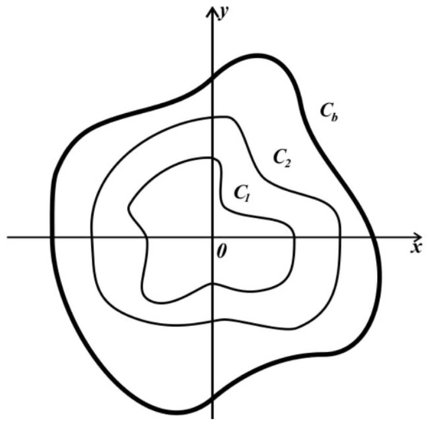
We see that the level lines of the equilibrium density play an important role in our analysis. Below, the density is assumed only to vary in a magnetic tube bounded by a simple smooth closed curve ${\mathcal{C}}_b$ (see Figure 1). Outside of the domain enclosed by ${\mathcal{C}}_b$, B is a constant, while $\rho$ can depend on z, but is independent of x and y. We define the Alfvén speed $V_A=B{\left({\mu }_0\rho \right)}^{-1/2}$, which can be rewritten as $V_A={\kappa }^{-1/2}\left(z\right)V_0(x,y)$, where $V_0=B{\left({\mu }_0{\rho }_0\right)}^{-1/2}$. $V_0$ is also a function of ${\rho }_0$ (or vice versa). Below, it is assumed that the level lines of $V_0$ constitute a nested set of simple smooth closed curves. This means that any level line is a smooth curve without intersection, and any two level lines do not intersect. The only exception is the central line. It can be either a dot or a not-closed line without intersection. When it represents a point, then we put the coordinate origin at this point; otherwise, the coordinate origin is put at one of the points along the central line. We prescribe a number $\psi \left(\mathcal{C}\right)$ to any level line $\mathcal{C}$ in such a way that $\psi =0$ at the central line and $\psi \left({\mathcal{C}}_1\right)<\psi \left({\mathcal{C}}_2\right)$ if the level line ${\mathcal{C}}_1$ occurs inside the level line ${\mathcal{C}}_2$; see Figure 1. If the notation ${\psi }_b\equiv \psi \left({\mathcal{C}}_b\right)$ is used, then, $\psi \in [0,{\psi }_b]$.

Now, let us introduce curvilinear orthogonal coordinates in the $xy$ plane as follows. One of these coordinates is $\psi$. The second coordinate is $\varphi$, defined by the condition that the system of curvilinear coordinates $\varphi$ and $\psi$ is orthogonal,

$$\frac{\partial \varphi }{\partial x}=\chi \frac{\partial \psi }{\partial y},\frac{\partial \varphi }{\partial y}=-\chi \frac{\partial \psi }{\partial x}.$$

(11)

The function $\chi$ is defined by the compatibility condition for the system of equations in Equation (11):

$$\frac{\partial \psi }{\partial x}\frac{\partial \chi }{\partial x}+\frac{\partial \psi }{\partial y}\frac{\partial \chi }{\partial y}+\chi \left(\frac{{\partial }^2\psi }{\partial x^2}+\frac{{\partial }^2\psi }{\partial y^2}\right)=0.$$

(12)

We make $\chi$ to be non-dimensional. Then, $\varphi$ is also non-dimensional. The $\varphi$-coordinate lines are defined by the condition $\psi =\mathrm{const}$ and coincide with the level lines of $V_0$, which implies that $V_0$ is independent of $\varphi$. The $\psi$-coordinate lines are defined by the condition $\varphi =\mathrm{const}$. They are orthogonal to the level lines of $V_0$. The Jacobian of transformation from coordinates $x,y$ to $\varphi ,\psi$ is

$$J=\left|\begin{array}{cc}\hfill {\displaystyle \frac{\partial \varphi }{\partial x}}& \hfill {\displaystyle \frac{\partial \varphi }{\partial y}}\\ \hfill {\displaystyle \frac{\partial \psi }{\partial x}}& \hfill {\displaystyle \frac{\partial \psi }{\partial y}}\end{array}\right|=\chi H^2,H^2={\left(\frac{\partial \psi }{\partial x}\right)}^2+{\left(\frac{\partial \psi }{\partial y}\right)}^2.$$

(13)

We assume that $\chi \ne 0$ everywhere. Since $-\chi$ is a solution to Equation (12) if $\chi$ is a solution, one can always have $\chi >0$. From the definition of $\psi$, it follows that the gradient of $\psi$ is orthogonal to the level lines of $V_0(x,y)$ and not equal to zero anywhere except the central line, that is, $H\ne 0$. Then, one concludes that $J>0$ everywhere but on the central line, and the curvilinear coordinates are right-oriented. Since $v$ and $\mathit{b}$ are tangent to the $\varphi$-coordinate lines that coincide with the level lines of $V_0$, both $v$ and $\mathit{b}$ have only $\varphi$-component. In accordance with this, the new variables u and w are introduced:

$$v=uH{\mathit{e}}_{\varphi },\mathit{b}=wH{\mathit{e}}_{\varphi },{\mathit{e}}_{\varphi }=\frac{1}{H}\left({\mathit{e}}_x\frac{\partial \psi }{\partial y}-{\mathit{e}}_y\frac{\partial \psi }{\partial x}\right),$$

(14)

where ${\mathit{e}}_x$ and ${\mathit{e}}_y$ are the unit vectors in the x and y-direction, respectively. Using Equations (13) and (14), one obtains:

$$\nabla ·v=\chi H^2\frac{\partial u}{\partial \varphi },$$

(15)

and a similar expression for $\nabla ·\mathit{b}$. Hence, the equations $\nabla ·v=0$ and $\nabla ·\mathit{b}=0$ reduce to the condition that u and w are independent of $\varphi$. Substituting expressions for $v$ and $\mathit{b}$, given by Equation (14), in Equation (7) yields:

$$\frac{\partial u}{\partial t}=\frac{B}{\rho {\mu }_0}\frac{\partial w}{\partial z},\frac{\partial w}{\partial t}=B\frac{\partial u}{\partial z}.$$

(16)

Let us recall that $\rho$ and, consequently, $V_A$, u, and w can depend on z. Equations (16) are quite similar to those in an axisymmetric equilibrium. The only difference is that in an axisymmetric equilibrium, u and w are the $\varphi$-components of the velocity and magnetic field perturbation, while in a non-axisymmetric equilibrium, the relation between the velocity and magnetic field perturbation and u and w is more involved and given by Equation (14). Finally, to note is that the Alfvén waves studied here do not disturb the tube boundary.

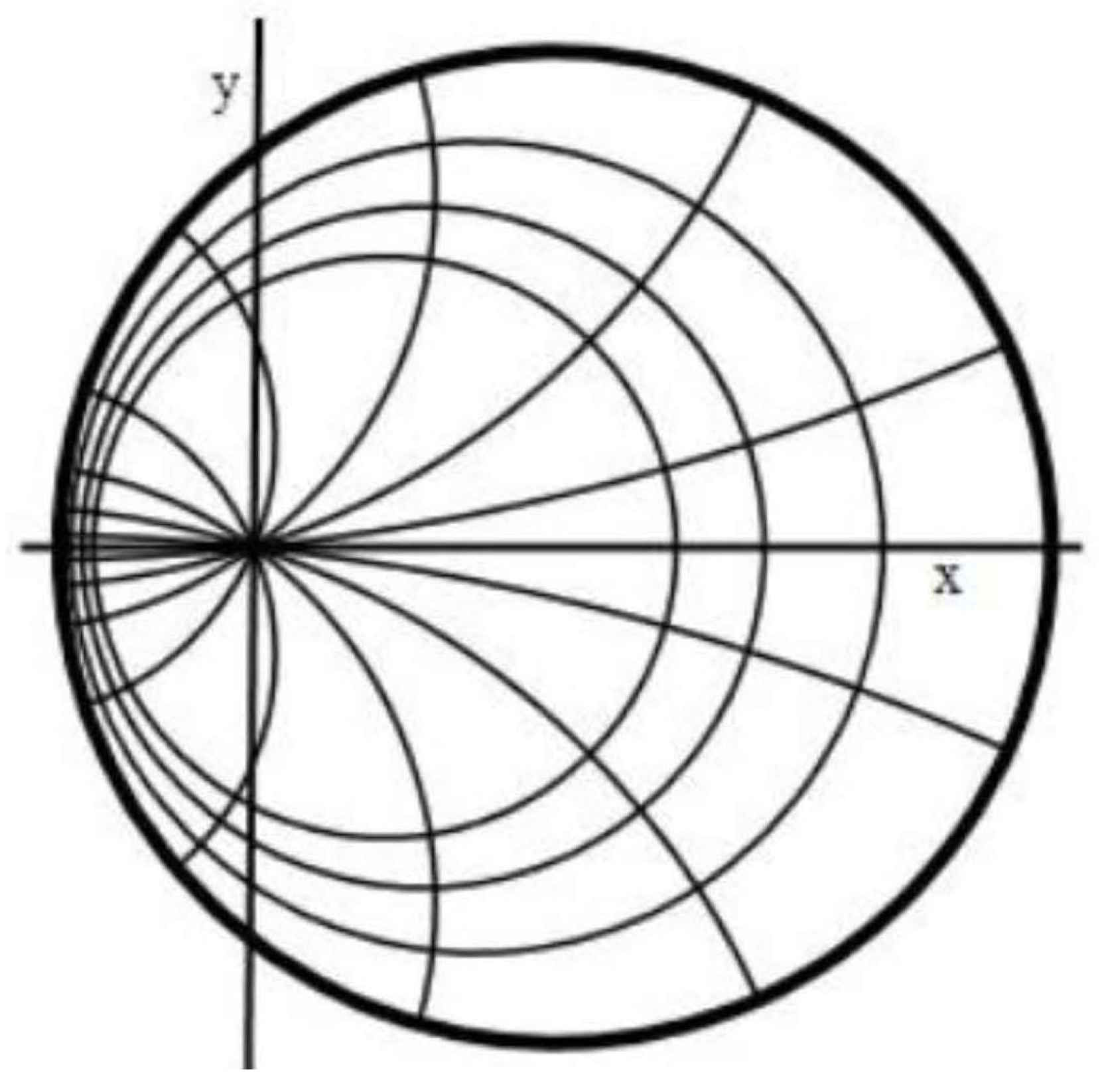
4. Example: Tube with Circular Cross-Section and Non-Axisymmetric Alfvén Speed Distribution

In order to make more clear the general results, obtained in Section 3, it is instructive to consider a particular example going step by step through the calculations made above. In this example, Alfvén waves are studied in a magnetic flux tube with a circular cross-section and non-axisymmetric Alfvén speed distribution. We use bi-cylindrical coordinates $\tau$ and $\sigma$ (e.g., [20]) (see Figure 2). Cartesian coordinates are expressed in terms of curvilinear coordinates as

$$x=\frac{asinh\tau }{cosh\tau -cos\sigma }-a,y=\frac{asin\sigma }{cosh\tau -cos\sigma },$$

(17)

where a is a constant with the dimension of length. The coordinate origin corresponds to $\tau \to \infty$. The tube boundary ${\mathcal{C}}_b$ is defined by $\tau ={\tau }_b$, and the tube interior is defined by $\tau >{\tau }_b$. In accordance with this, $\psi =1/\tau$. Hence, ${\psi }_b=1/{\tau }_b$. The tube radius is $a{(sinh{\tau }_b)}^{-1}$. The distance from the coordinate origin, r, is defined by

$$r^2=x^2+y^2=a^2\left(1+\frac{cosh\tau -2sinh\tau +cos\sigma }{cosh\tau -cos\sigma }\right).$$

(18)

Let us define the Alfvén speed in the plane $z=0$ as

$$V_0=V+(V_b-V){\left(\frac{sinh{\tau }_b}{sinh\tau }\right)}^2,$$

(19)

where $0<V<V_b$. One can see that $V_0$ is a monotonically decreasing function of $\tau$, which implies that it gets to a minimum at the coordinate origin. In addition, $V_0=V+(V_b-V){(r/a)}^2$ for $r\ll a$ what corresponds to $\tau \gg 1$. Hence, $V_0$ is a continuously differentiable function in the region bounded by ${\mathcal{C}}_b$. Using Equation (17), one obtains:

$$\begin{array}{c}{\displaystyle \frac{\partial f}{\partial x}=-\frac{1}{a}\frac{\partial f}{\partial \tau }(cosh\tau cos\sigma -1)-\frac{1}{a}\frac{\partial f}{\partial \sigma }sinh\tau sin\sigma ,}\hfill \\ {\displaystyle \frac{\partial f}{\partial y}=-\frac{1}{a}\frac{\partial f}{\partial \tau }sinh\tau sin\sigma +\frac{1}{a}\frac{\partial f}{\partial \sigma }(cosh\tau cos\sigma -1),}\hfill \end{array}$$

(20)

where f is a continuously differentiable function. Using Equation (20), the formula [20],

$${\nabla }^{2}f=\frac{1}{a^2}{(cosh\tau -cos\sigma )}^2\left(\frac{{\partial }^{2}f}{\partial {\sigma }^2}+\frac{{\partial }^{2}f}{\partial {\tau }^2}\right),$$

(21)

and taking into account that $\psi$ is independent of $\sigma$, Equation (12) reads:

$$\frac{\partial }{\partial \tau }\left(\chi \frac{d\psi }{d\tau }\right)=0.$$

(22)

Using Equation (19), one obtains that a particular solution to this equation is $\chi ={\tau }^2$. With this result and Equation (20), one obtains from Equation (11):

$$\begin{array}{c}{\displaystyle \frac{\partial \varphi }{\partial \tau }(cosh\tau cos\sigma -1)+\frac{\partial \varphi }{\partial \sigma }sinh\tau sin\sigma =-sinh\tau sin\sigma ,}\hfill \\ {\displaystyle \frac{\partial \varphi }{\partial \tau }sinh\tau sin\sigma -\frac{\partial \varphi }{\partial \sigma }(cosh\tau cos\sigma -1)=(cosh\tau cos\sigma -1).}\hfill \end{array}$$

(23)

From the system (23), it follows that

$$\frac{\partial \varphi }{\partial \tau }=0,\frac{\partial \varphi }{\partial \sigma }=-1.$$

(24)

These equations imply that one can take $\varphi =-\sigma$. Although we found the expressions for $\psi$ and $\varphi$, it is more convenient to use $\tau$ and $\sigma$ in this particular example. Using Equations (13) and (20):

$$H=\frac{cosh\tau -cos\sigma }{a{\tau }^2}.$$

(25)

Finally, ${\mathit{e}}_{\varphi }=-{\mathit{e}}_{\sigma }$. It is interesting to compare the maximum and minimum values of the speed at the level line $\tau =\mathrm{const}$. Since u is independent of $\sigma$, it follows from Equations (14) and (25) that the ratio of these quantities is

$$\frac{{\left|v\right|}_{\max }}{{\left|v\right|}_{\min }}=\frac{cosh\tau +1}{cosh\tau -1}.$$

(26)

One can see that this ratio increases with the distance from the coordinate origin and can be large far from it, what is for sufficiently small values of $\tau$.

5. Summary and Conclusions

In this paper, torsional Alfvén waves were studied in a magnetic flux tube with an arbitrary cross-section. We assumed that the magnetic field is propagating in the z-direction in Cartesian coordinates $x,y,$ and z. The tube cross-section is bounded by a smooth closed curve. Both the plasma pressure and the magnetic field are homogeneous outside this curve, while the plasma density still can vary in the z-direction. Inside the tube, all equilibrium quantities can depend on x and y. The density can also depend on z; however, it can be factorised and expressed as a product of two functions: one dependent on x and y and the other dependent on z. Hence, the same is valid for the Alfvén speed $V_A$: that is, it can be expressed as a product of a function dependent on z and $V_0(x,y)$. It is assumed that the level lines of $V_0(x,y)$ are smooth closed curves and constitute a nested set of curves. The only exception is the central curve that is either a point or a not closed line without self-intersections. We introduced an orthogonal curvilinear coordinate system with one of the two curvilinear coordinates being constant on the level lines of $V_0(x,y)$. This coordinate is zero at the central line and has the following property: If a level line ${\mathcal{C}}_1$ is inside a level line ${\mathcal{C}}_2$, then this coordinate is smaller on ${\mathcal{C}}_1$ than on ${\mathcal{C}}_2$.

Here, Alfvén waves were defined as waves that do not disturb plasma density. We showed that these waves can exist only when the magnetic field magnitude is a function of $V_0$. We consider this as the main result of the paper. When the condition of existence of Alfvén waves is satisfied, the latter are polarised in the directions been orthogonal to the magnetic field and tangent to the level lines of $V_0$. The wave amplitude varies along the level lines of $V_0$. As an example, torsional Alfvén waves in a magnetic tube with a circular cross-section but non-axisymmetric distribution of the Alfvén speed were studied.