Article

SIR-Solution for Slowly Time-Dependent Ratio between Recovery and Infection Rates

by
Martin Kröger
1,* and
Reinhard Schlickeiser
2,3,*
1
Polymer Physics, Department of Materials, ETH Zurich, CH-8093 Zurich, Switzerland
2
Theoretische Physik, Weltraum- und Astrophysik, Lehrstuhl IV, Ruhr-Universität Bochum, D-44780 Bochum, Germany
3
Institut für Theoretische Physik und Astrophysik, Christian-Albrechts-Universität zu Kiel, Leibnizstr. 15, D-24118 Kiel, Germany
*
Authors to whom correspondence should be addressed.
Physics 2022, 4(2), 504-524; https://doi.org/10.3390/physics4020034
Submission received: 27 February 2022 / Revised: 20 April 2022 / Accepted: 26 April 2022 / Published: 9 May 2022
(This article belongs to the Special Issue Physics Methods in Coronavirus Pandemic Analysis)

Abstract

:
The temporal evolution of pandemics described by the susceptible-infectious-recovered (SIR)-compartment model is sensitively determined by the time dependence of the infection ( a ( t ) ) and recovery ( μ ( t ) ) rates regulating the transitions from the susceptible to the infected and from the infected to the recovered compartment, respectively. Here, approximated SIR solutions for different time dependencies of the infection and recovery rates are derived which are based on the adiabatic approximation assuming time-dependent ratios, k ( t ) = μ ( t ) / a ( t ) , varying slowly in comparison with the typical time characteristics of the pandemic wave. For such slow variations, the available analytical approximations from the KSSIR-model, developed by us and valid for a stationary value of the ratio k, are used to insert a posteriori the adopted time-dependent ratio of the two rates. Instead of investigating endless different combinations of the time dependencies of the two rates a ( t ) and μ ( t ) , a suitably parameterized reduced time, τ , dependence of the ratio k ( τ ) is adopted. Together with the definition of the reduced time, this parameterized ratio k ( τ ) allows us to cover a great variety of different time dependencies of the infection and recovery rates. The agreement between the solutions from the adiabatic approximation in its four different studied variants and the exact numerical solutions of the SIR-equations is tolerable providing confidence in the accuracy of the proposed adiabatic approximation.

1. Introduction

About a century ago, the susceptible-infectious-recovered/removed (SIR) model was introduced [1] to the mathematical theory of epidemics. Together with later improvements [2], it represents the fundamental compartment model where any considered population of N persons is divided into the three fractions of susceptible (S), infected (I) and recovered/removed (R) persons. The infection rate, a ( t ) , and the recovery/removed rate, μ ( t ) , regulate the transitions from the susceptible to the infected compartment and from the infected to the recovered/removed compartment, respectively. The original SIR model has been generalized to a more complicated version, adding additional compartments such as the fraction of exposed persons (for reviews, see [3,4]) and vaccinated persons [5], and widely applied to epidemic outbreaks including COVID-19 and SARS-CoV-2 [6].
Very often, the SIR equations are solved numerically with adopted stationary infection ( a 0 ) and recovery ( μ 0 ) rates so that their ratio, k = μ 0 / a 0 , is also constant and stationary, although an analytical solution in terms of an inverse integral of this case has been known since 2014 [7].
Analytical solutions for arbitrary but given time dependencies of the infection rate a ( t ) have been derived recently [8,9] for the infinite time domain and the semi-time time domain for the case of a stationary ratio k = μ ( t ) / a ( t ) , implying that the recovery rate has exactly the same time dependence as the infection rate. Hereafter, these generalizations are referred to as the KSSIR-model. This generalization to a time-dependent infection rate is important as such time dependencies are caused by non-pharmaceutical interventions (NPIs) taken during pandemic outbreaks. In the KSSIR-model [8,9], exact analytical inverse solutions t ( Q ) for all relevant quantities Q [ S , I , R ] in terms of Lambert functions were obtained. These inverse solutions were approximated with high accuracy yielding the explicit time dependencies Q ( t ) by inverting the Lambert functions. Of particular importance are the obtained analytical expressions for the peak time and asymptotic behaviors, early doubling times, late half-decay time of the rate of new infections, J ˙ ( t ) = d J / d t = a ( t ) S ( t ) I ( t ) , and its corresponding cumulative number J ( t ) , which allowed the quantitative comparison with the monitored temporal evolution of different waves the COVID-19 [10] and the forecast for the omicron mutant [11].
It is the purpose of the present paper to investigate analytical solutions of the SIR equations for different time dependencies of the infection and recovery rates so that their ratio no longer is constant and becomes also time-dependent. To the best of our knowledge, this general case has not been studied in the literature apart from [12], in which were studied special analytical solutions based on non-constant ratios, k ( S ) , being of polynomial form of order S 4 or less in the case of positive or negative powers. However, in this paper, no relations to monitored pandemic parameters were established.
Here, a different approach is considered by investigating the adiabatic case which refers to slowly varying (in comparison to the typical time characteristics of the pandemic wave) time-dependent ratios k ( t ) . The adiabatic approximation [13,14] is an established known method in theoretical physics, especially semi-classical quantum mechanics see, e.g., the WKBJ-method [15,16,17,18] for slowly varying potentials or the Born–Oppenheimer approximation [19] for the analysis of molecules. The latter simplifies the solution of the quantum mechanical equations of motion by taking advantage of the drastically different time scales of motion of the light and heavy particles in the system. Thus, for the analysis below for slow variations of the function k ( t ) , the available analytical approximations from the KSSIR-model (which strictly are valid only for constant ratios k) is used here and the adopted time-dependent ratio k ( t ) is inserted a posteriori. The resulting adiabatic solutions is then compared to the exact numerical solutions of the SIR-equations for given time variations of k ( t ) .

2. Starting Equations

The general dynamical SIR equations for the fractions of susceptible, infectious, and recovered/removed compartments are:
S ˙ ( t ) = a ( t ) S ( t ) I ( t ) , I ˙ ( t ) = a ( t ) S ( t ) I ( t ) μ ( t ) I ( t ) , R ˙ ( t ) = μ ( t ) I ( t ) ,
which obey the sum constraint,
S ( t ) + I ( t ) + R ( t ) = 1 .
Here, the semi-time case (as opposed to the all-time case treated in [2,8,20]) with the initial conditions I ( t = t 0 ) = η , S ( t = t 0 ) = 1 η , and R ( t = t 0 ) = 0 is considered. It is convenient to introduce the reduced time variable,
τ = t 0 t d y a ( y ) ,
which can be calculated for any given time dependence of the infection rate a ( t ) . Equation (1) then read:
d I d τ = S I k ( τ ) I , d S d τ = S I , d R d τ = k ( τ ) I ,
in terms of the dimensionless, time-dependent ratio of infection to recovery rate,
k ( τ ( t ) ) = μ ( t ( τ ) ) a ( t ( τ ) ) .
There are no obvious natural choices for the real time dependencies of the infection and the recovery rates, and they may differ from mutant to mutant. Initially, at the start of the mutant outbreak, without any taken NPIs, the rates have the values a ( t 0 ) = a 0 and μ ( t 0 ) = μ 0 . Dedicated medication of infected persons certainly will increase the recovery rate from its initial value, whereas the NPIs [21,22,23,24,25,26,27,28,29] (such as social distancing, quarantining and mask obligations) effectively reduce the infection rate from its initial value.
Instead of investigating endless different combinations of the time dependencies of the rates a ( t ) and μ ( t ) , a different approach is followed here by adopting a suitably parameterized reduced time dependence of the ratio k ( τ ) . Along with Equation (3), holding for any given real time dependence of the infection rate a ( t ) , one is then able to represent quite a variety of different real time dependencies of the infection and recovery rates as detailed in Section 5. As suitably parameterized reduced time dependency
k ( τ ) = k 1 + k 1 k 0 1 + tanh ( τ c / Δ ) tanh τ τ c Δ 1
is adopted.
The function (6) starts from the value k 0 at the initial time τ = 0 and approaches the final value k 1 after infinite time τ = . As Figure 1 demonstrates, its parameters τ c and Δ regulate the sharpness of the transition from k 0 to k 1 . For small differences between the chosen initial ( k 0 ) and final ( k 1 ) values of the function k ( τ ) , the overall variation of this function is comparatively small. The last argument can be formulated more quantitatively. The function (6) has its strongest gradient,
d k d τ max = k 1 k 0 [ 1 + tanh ( τ c / Δ ) ] Δ
at τ = τ c so that its shortest relative variation time scale is given by
τ k , min = k ( τ c ) d k d τ max = k 0 + k 1 tanh ( τ c / Δ ) Δ | k 1 k 0 | > k 0 Δ | k 1 k 0 | ,
where the last lower limit holds because tanh ( τ c / Δ ) > 0 for all finite values of the parameters Δ and τ c . Quantitatively, a slowly varying function k ( τ ) means that the lower limit (8) of relative time scale is long compared to the typical relative time variation of the pandemic wave, which is characterized by its early doubling time (see Equation (68) in [8]), τ 2 = ( ln 2 ) / ( 1 k 0 ) , implying k 0 Δ / | k 1 k 0 | τ 2 , or
k 0 ( 1 k 0 ) Δ | k 1 k 0 | 0.693
as quantitative parameter requirement for the slowliness of the time variation of the function k ( τ ) . The time scale (8) increases inversely to the difference between the chosen initial and final values of the function k ( τ ) . For all examples considered below, the parameter requirement (9) is satisfied.
The functional form of Equation (6) was mainly chosen for its mathematical convenience and suitability. On the one hand, it is general enough to model all possible reasonable sorts of time-dependent ratios of infection to recovery rates: increasing or decreasing ones from an initial to a finite value with steep, modest or slow transitions. On the other hand, it is mathematically simple enough that it allows us exact analytical computations, as demonstrated, e.g., in Section 5 below.

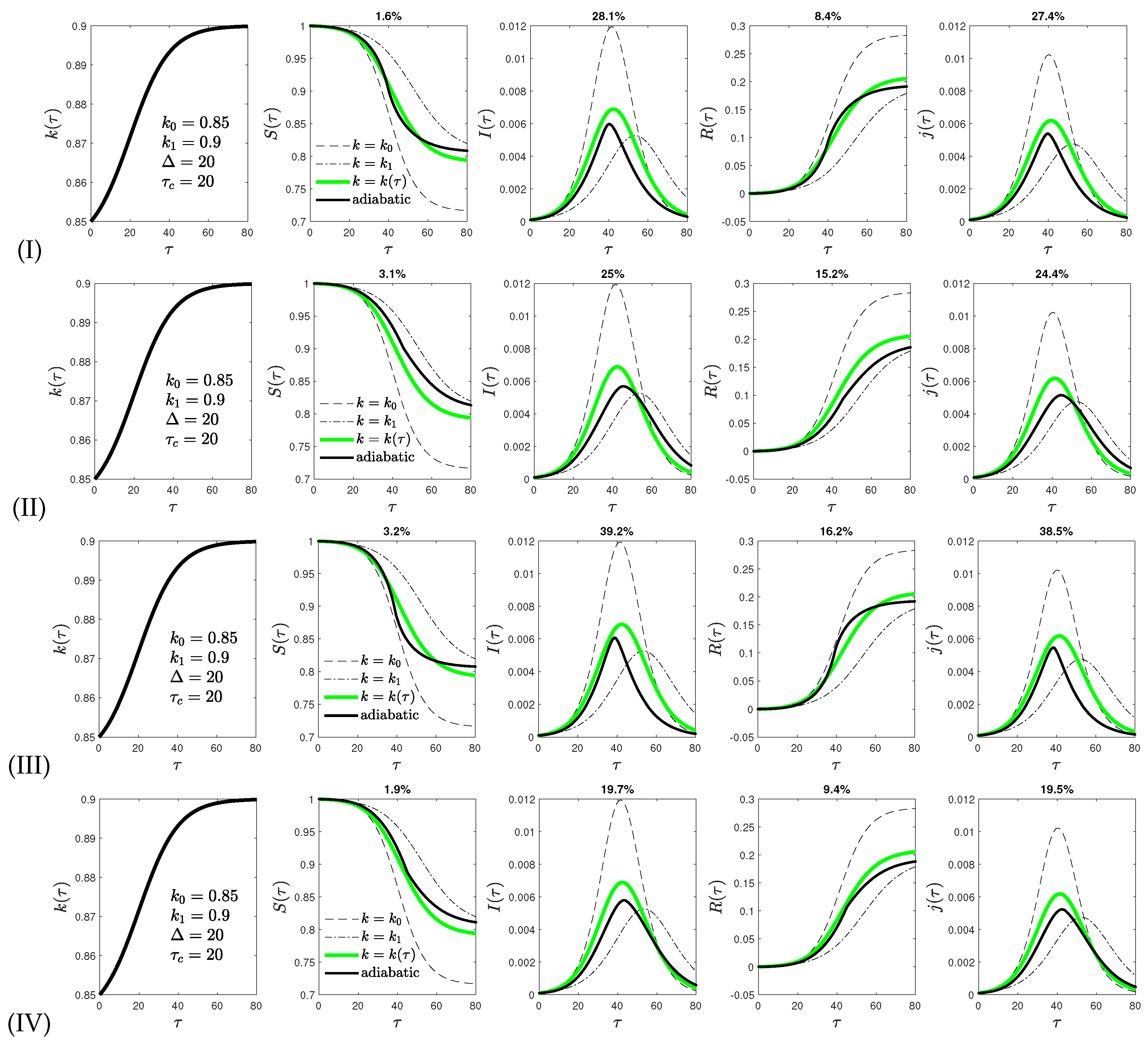
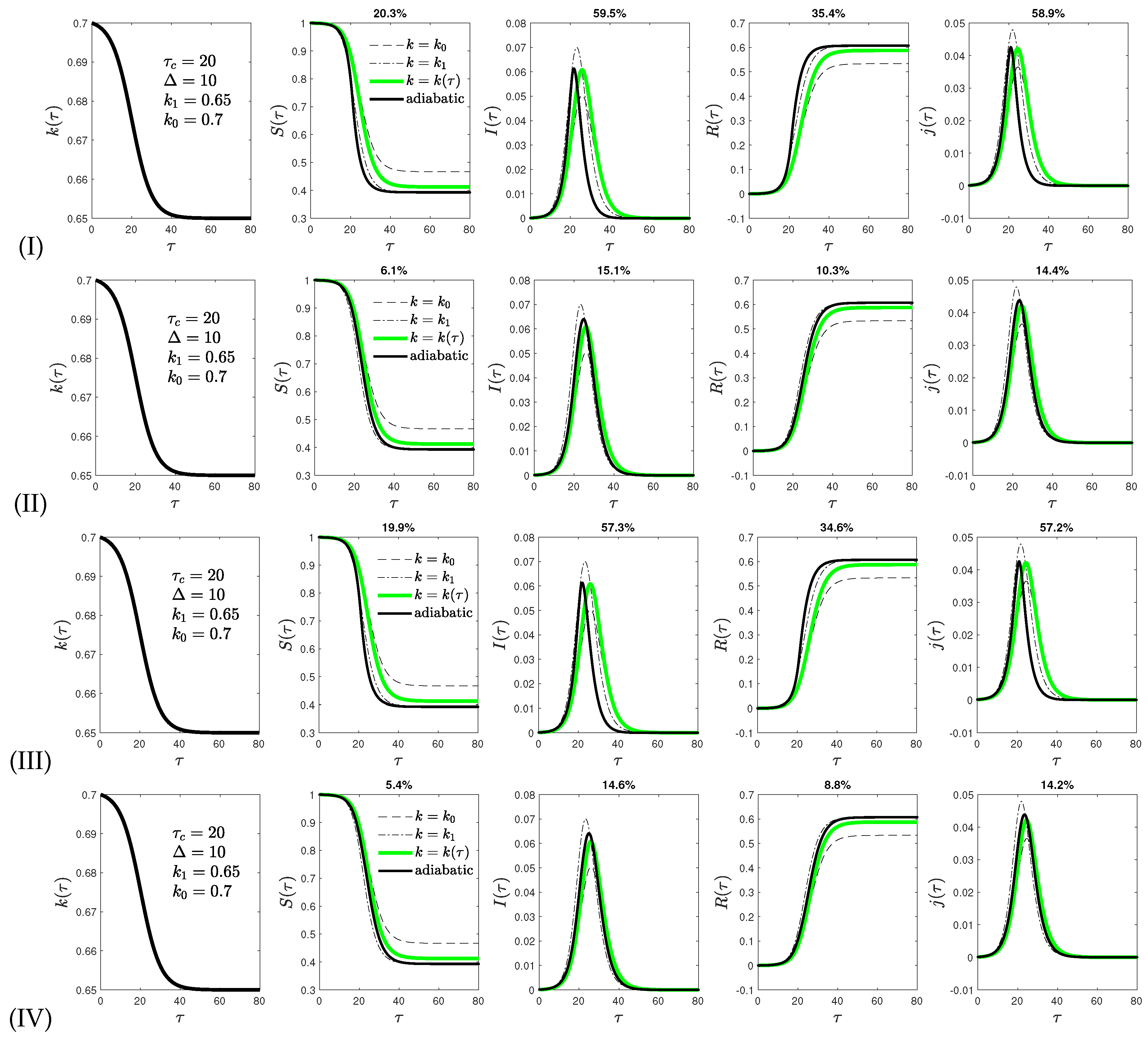
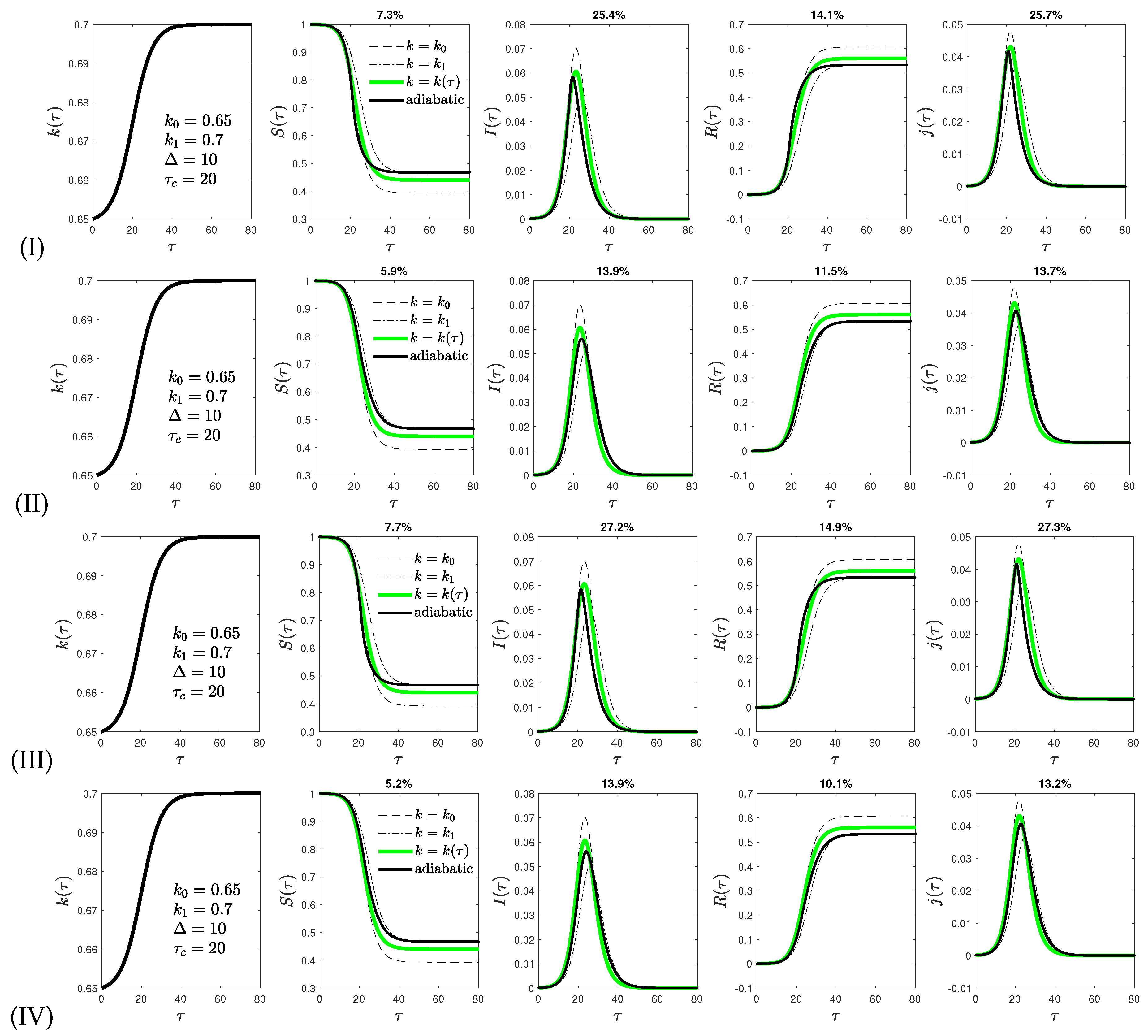
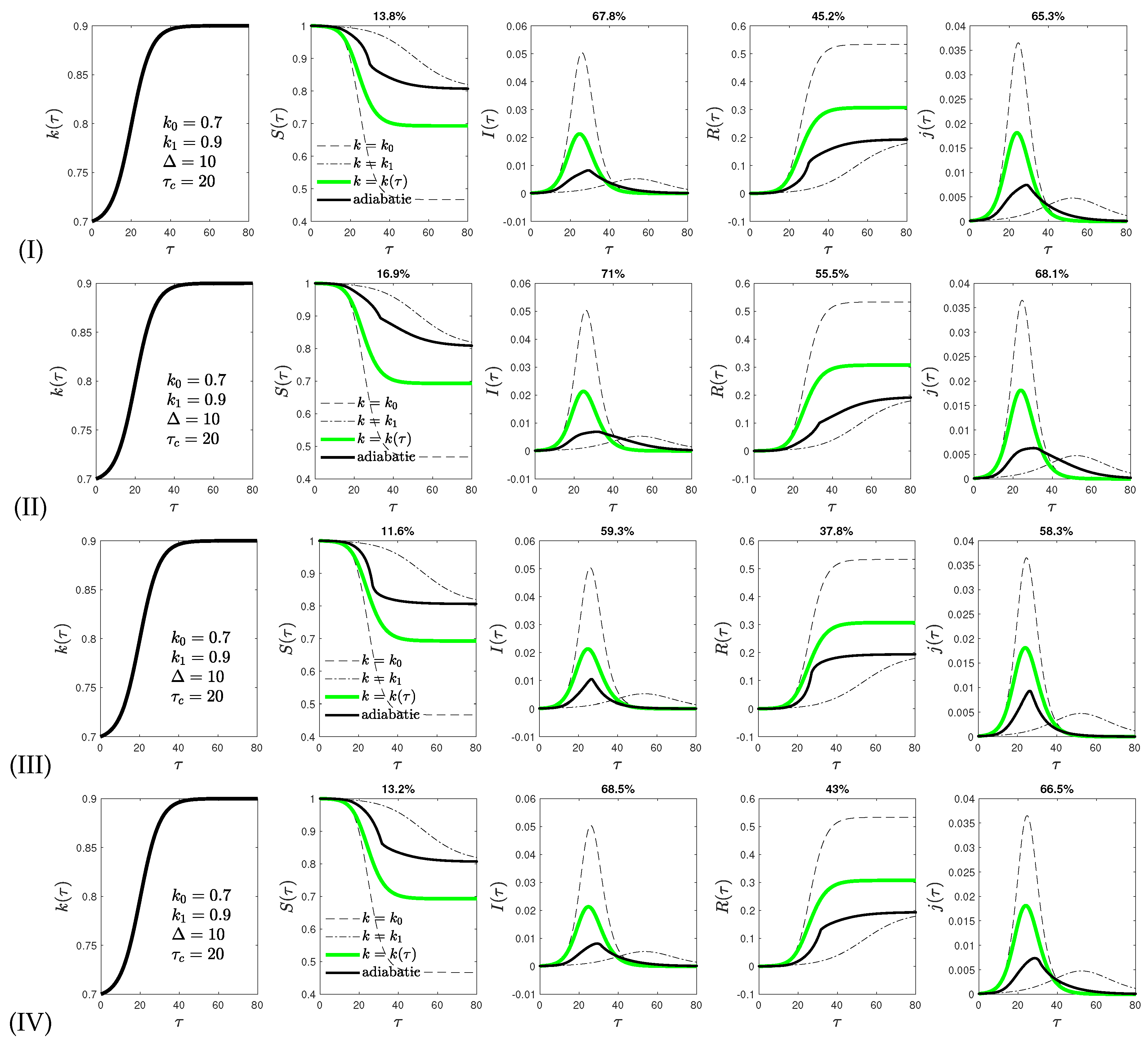
3. Analytical Adiabatic Approximations

Here, the exact and analytical results from the KSSIR model are used, as summarized in Section 2 of [11], and the reduced time dependence (6) is inserted a posteriori. Consequently, for this adiabatic approximation, one obtains that S ( τ ) = 1 J ( τ ) , I ( τ ) = J ( τ ) + k ( τ ) ϵ + k ( τ ) ln [ 1 J ( τ ) ] , R ( τ ) = k ( τ ) [ ϵ + ln ( 1 J ( τ ) ) ] with ϵ = ln ( 1 η ) in terms of the cumulative number of new infections, J ( τ ) . The latter is given by [10]
J ( τ ) η + J 0 ( k ) η 1 + j max ( k ) c 0 sinh [ c 3 ( τ ^ m τ ) ] sinh ( c 3 τ ) for τ τ ^ m , J ( k 1 ) J ( k 1 ) J 0 ( k ) j max ( k ) c 4 J ( k 1 ) J 0 ( k ) exp [ c 4 ( τ τ ^ m ) ] 1 + 1 for τ τ ^ m ,
where k, c 3 and c 4 stand for k ( τ ) , c 3 ( k ( τ ) ) and c 4 ( k ( τ ) ) . The interpolated dimensionless peak time is given by
τ ^ m = 2 τ m 1 ( k 0 ) + τ m 1 ( k 1 ) , τ m ( k ) = 1 c 3 ( k ) artanh 2 c 3 ( k ) c 1 ( k ) + 2 c 0 J 0 ( k ) η ,
and the abbreviations
c 0 = η ( 1 η ) , c 1 ( k ) = 1 k 2 η , c 2 ( k ) = j max ( k ) c 0 c 1 ( k ) [ J 0 ( k ) η ] [ J 0 ( k ) η ] 2 , c 3 ( k ) = c 1 ( k ) 2 2 c 0 c 2 ( k ) , c 4 ( k ) = J ( k 1 ) ( 1 k ) .
Here,
j max ( k ) = k 2 4 1 + W 1 2 ( 1 η ) k exp ( 1 + 1 / k ) 2 1
denotes the maximum rate of new infections occurring at
J 0 ( k ) = 1 + k 2 W 1 2 ( 1 η ) k exp ( 1 + 1 / k ) ,
and
J ( k 1 ) = lim τ J ( τ ) 1 + k 1 W 0 1 η k 1 e 1 / k 1
is the final cumulative fraction of infected persons. Equations (13)–(15) depend on the principal ( W 0 ) and non-principal ( W 1 ) solution of Lambert’s equation [8], the known and documented Lambert functions. Let us emphasize that for small values of η 1 , the results (13)–(15) are basically independent of the value of η and only determined by the ratio k ( τ ) .
The reduced time dependence of the rate of new infections in the adiabatic case is then given by
j ( τ ) [ 1 J ( τ ) ] [ J ( τ ) + k ( τ ) ϵ + k ( τ ) ln ( 1 J ) ] .
Throughout this paper, Equations (11)–(16) will be referred to as
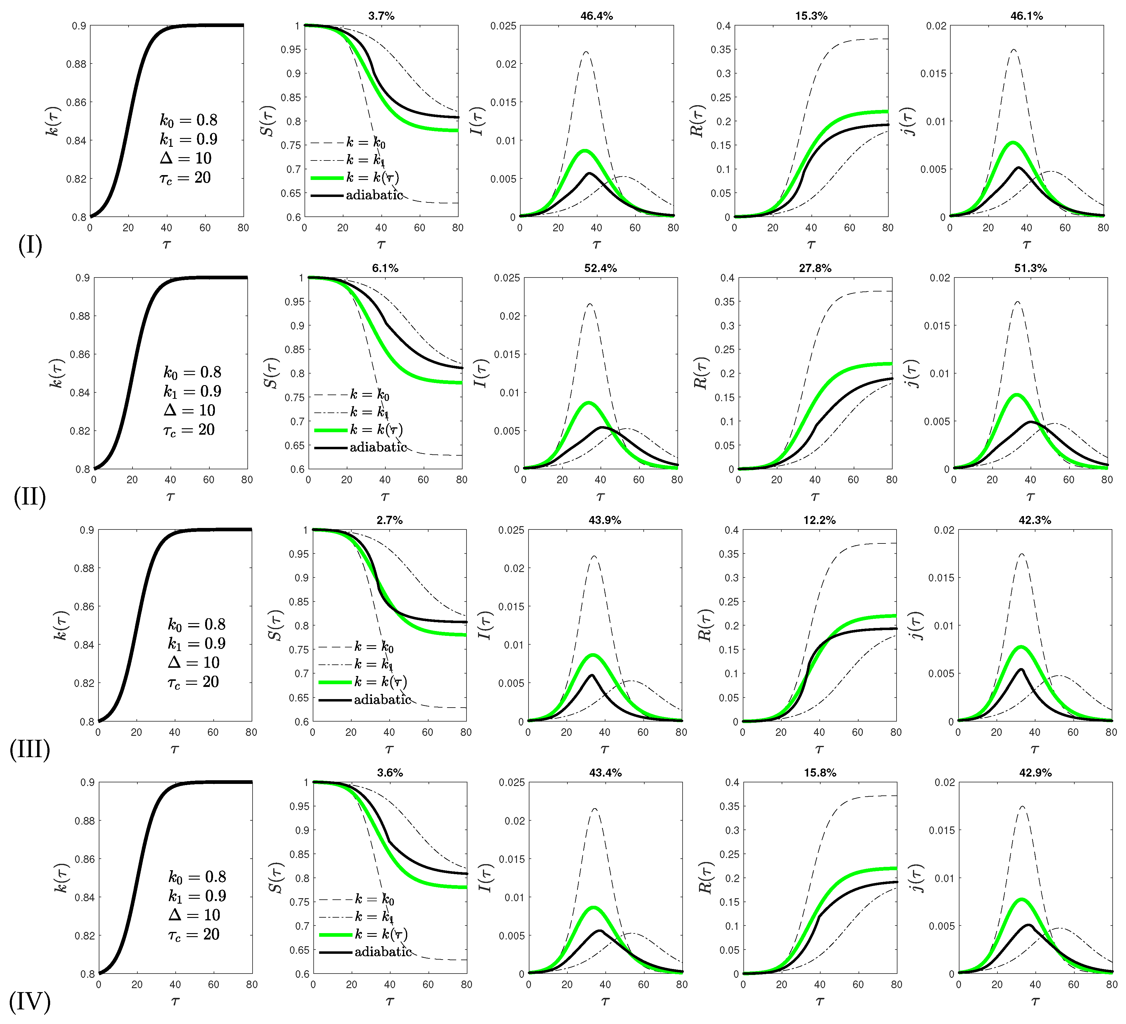
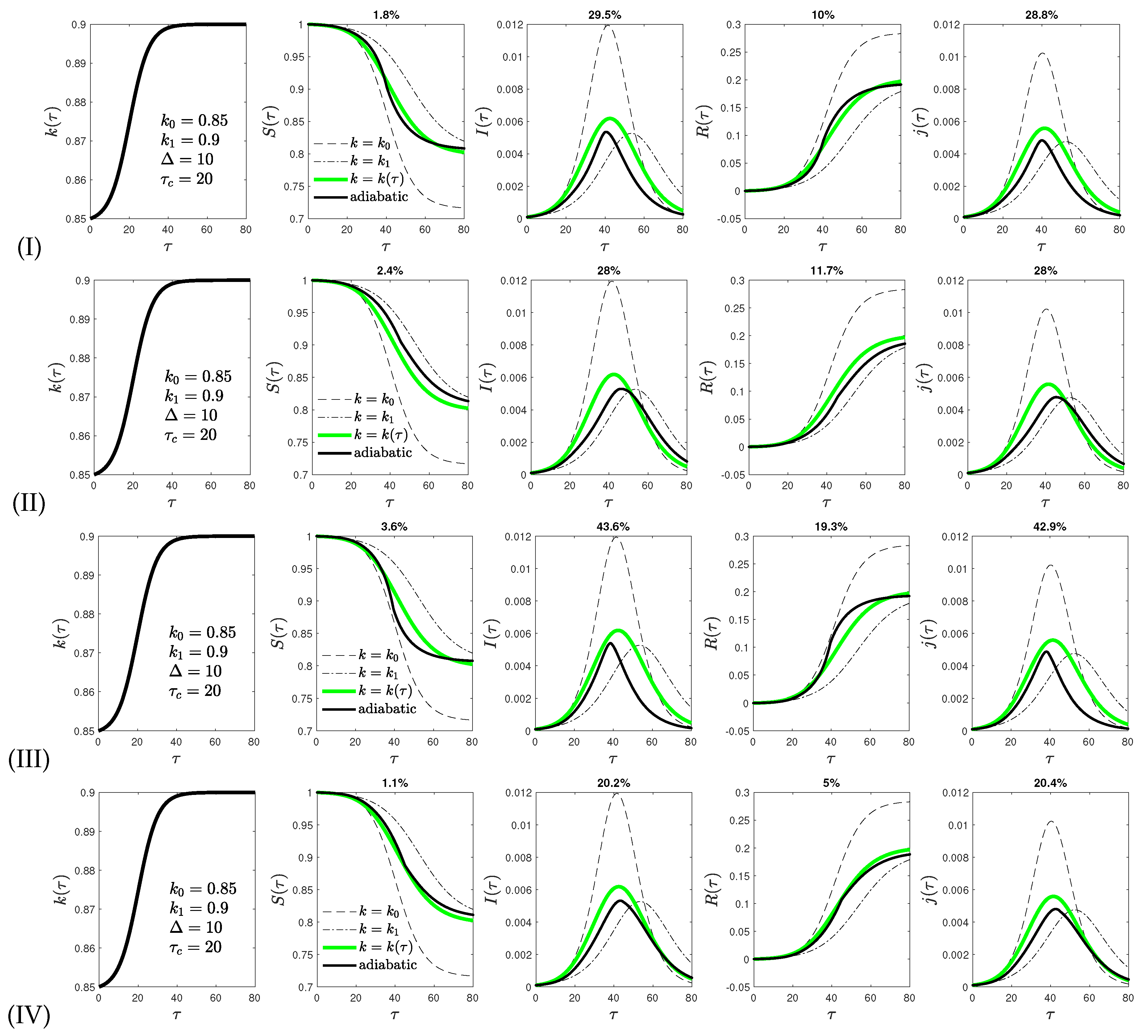
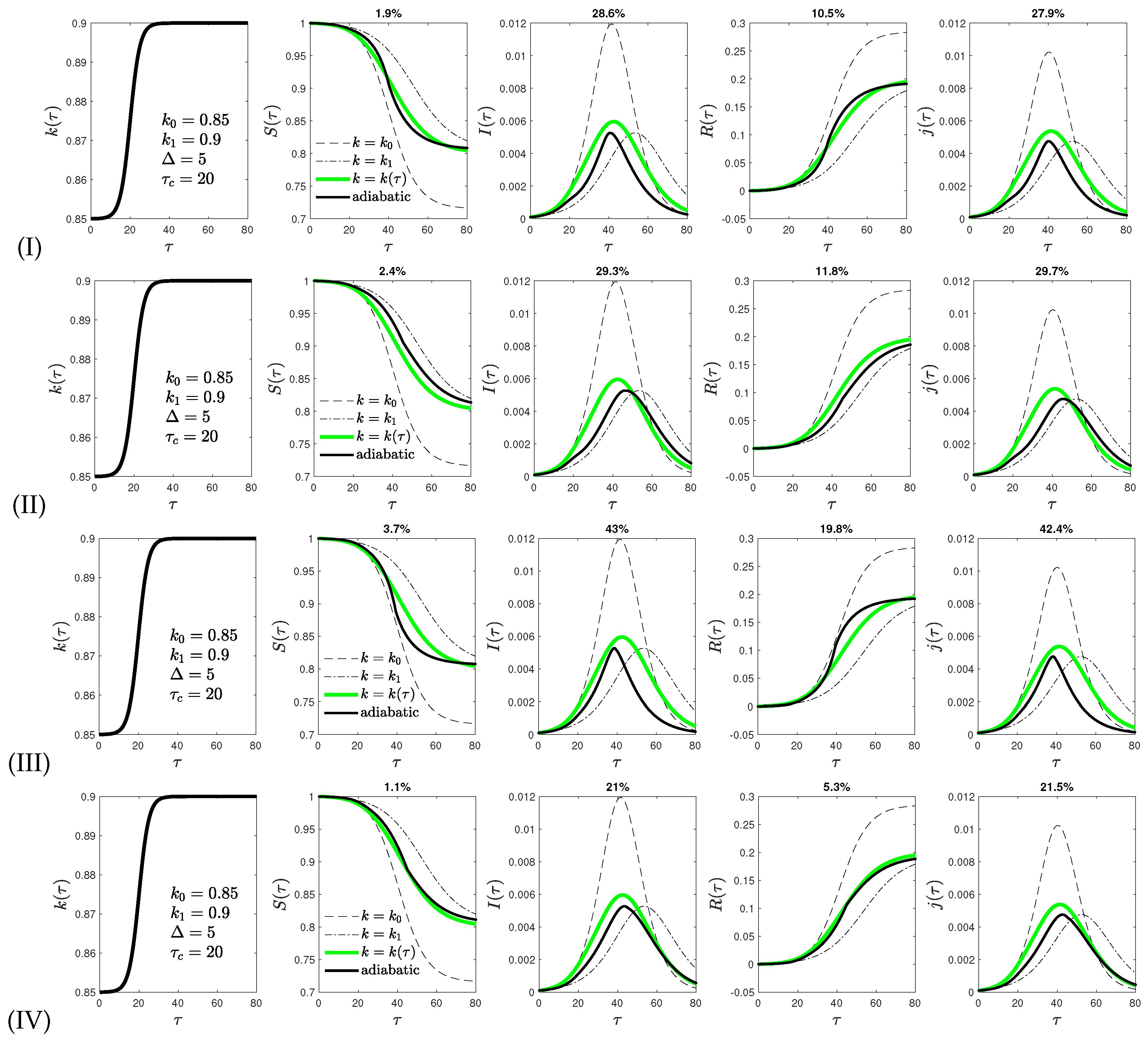
  • version I of the adiabatic analytical approximation. Additionally, three slightly different versions of this model are investigated, named versions II to IV.
  • In version II, the j max are calculated not using their own Equation (13) but Equation (16) where J is replaced by J 0 from Equation (14).
  • For version III,
    J 0 ^ = 2 [ J 0 1 ( k 0 ) + J 0 1 ( k 1 ) ]
    is used instead of J 0 ( k ) in Equation (14) within the spirit of the interpolated τ ^ m in Equation (11). This appears more consistent, as τ ^ m belongs to the value of J 0 .
  • Version IV combines versions II and III.

4. Comparison of Analytical and Exact Results in Reduced Time

Figure 2, Figure 3, Figure 4, Figure 5, Figure 6, Figure 7 and Figure 8 compare the exact numerical solutions with the four versions of the analytical adiabatic approximations for different parameter choices of the reduced time dependence of the ratio (6), the fractions S, I, and R, and the rate of new injections (16). The numerical solution is obtained using a solver for moderately stiff ordinary differential equations, as proposed earlier [30]. To this end, the trapezoidal rule is applied using a “free” interpolant [31,32]. Note that in Figure 6, a decreasing ratio (6) with reduced time is chosen, whereas in Figure 2, Figure 3, Figure 4 and Figure 5, Figure 7, and Figure 8, increasing ratios are considered.
As expected, in every case, both the exact numerical curve and the adiabatic approximation initially at small reduced times are close to the KSSIR-behavior for the value k 0 , whereas at late times, these two curves approximate the KSSIR-behavior for the final value k 1 .
The agreement between the exact numerical reduced time and the adiabatic approximation reduced time dependence in all four versions is tolerable. In the worst case, the maximum deviation is 68.1%, but in most shown examples—much less. This acceptable agreement provides confidence in the accuracy of the proposed adiabatic approximation, but certainly leaves room for future improvement.
As it looks, there are no strong differences in the four versions of the adiabatic approximation. However, placing the greatest emphasis on the rates of new infections j ( τ ) , as these can be compared with the monitored pandemic data in different countries and societies, version IV of the adiabatic approximation gives the most accurate analytical results, and therefore may be favored over the other three versions. Regarding the rate j ( τ ) the maximum deviation increases roughly as 400 | k 1 k 0 | percent with greater differences in the final and initial values of the function k ( τ ) .

5. Relation between the Reduced and Real Time Dependence of the Infection and Recovery Rate

In order to calculate the real time dependence from the reduced time dependence of the SIR-quantities of interest, one has to infer the real time dependencies of the infection and recovery rates from the adopted parameterized reduced time dependence (6) of their ratio. Two different cases to be considered: in the first case, a real time dependence of the infection rate a ( t ) is adopted, whereas in the second case, the real time dependence of the recovery rate μ ( t ) is pre-specified. If in the first case a constant infection rate for all real times is adopted, the entire real time variation of the ratio k ( t ) stems from the recovery rate. Likewise, if in the second case a constant recovery rate at all real times is pre-specified, the real time variation of the rate k ( t ) results from the infection rate. Below, each case is considered in turn.

5.1. Case 1: Pre-Specified Infection Rate

In this case, one starts from constant infection rate a ( t ) = a 0 at all times. Then, Equation (3) yields for the reduced time τ = a 0 ( t t 0 ) . Consequently, Equations (5) and (6) provide for the real time dependence of the recovery rate, i.e.,
μ ( t ) = a 0 k ( a 0 ( t t 0 ) ) = a 0 k 1 + k 1 k 0 1 + tanh ( τ c / Δ ) tanh a 0 ( t t 0 ) τ c Δ 1 .
For values k 1 > k 0 , Equation (18) indeed represents an increase of the recovery rate which can be either slow or rapid depending on the chosen parameters Δ and τ c .
As a second example of a pre-specified infection rate, the earlier considered lockdown infection rate [33],
a LD ( t ) = a 0 2 1 + q ( 1 q ) tanh t t 0 t a t b a 0 for t 0 t t a , q a 0 for t t a ,
is used employing a quarantine factor, q [ 0 , 1 ] , which implies
τ LD ( t ) = a 0 2 ( 1 + q ) ( t t 0 ) ( 1 q ) t b ln cosh t t 0 t a t b cosh t a / t b a 0 ( t t 0 ) for t 0 t t a , q a 0 t for t t a .
The time-dependent infection rate (19) has been studied before [33] to describe the effect of lockdown interventions on the temporal evolution of pandemic waves. The function (19) is characterized by four parameters: (i) the initial constant infection rate a 0 at early times t t a , (ii) the final constant infection rate a 1 = q a 0 at late times t t a described by the quarantine factor q = a 1 / a 0 1 , (iii) the time t a of maximum change, and (iv) the time t b t a regularizing the sharpness of the transition. The latter is known to be about t b 7 days reflecting the typical one week incubation delay.
Upon insertion of a LD ( t ) and τ LD ( t ) Equations (5) and (6) then yield for the real time dependence of the recovery rate:
μ LD ( t ) = a LD ( t ) k ( τ LD ( t ) ) .
Figure 9 shows the resulting real time dependence of the recovery rate for the adopted lockdown infection rate.

5.2. Case 2: Pre-Specified Recovery Rate

The second case of a pre-specified recovery rate is more complex. Starting again from a constant recovery rate μ ( t ) = μ 0 , Equations (3), (5) and (6) then yield for the real time dependence of the infection rate the implicit integral equation,
a ( t ) = μ 0 k 1 + k 1 k 0 1 + tanh ( τ c / Δ ) tanh t 0 t a ( y ) d y τ c Δ 1 .
Introducing
Y ( t ) = t 0 t a ( y ) d y τ c Δ = τ τ c Δ ,
so that d Y / d t = a ( t ) / Δ , and the abbreviation
K = k 1 k 0 1 + tanh ( τ c Δ ) ,
Equation (22) reads:
k 1 K + K tanh Y d Y d t = μ 0 Δ .
Integrating Equation (25) then readily yields:
( k 1 k ) Y ( t ) + K ln cosh Y ( t ) = μ 0 Δ t + c 1 .
With the initial value, Y ( t 0 ) = τ c / Δ , one obtains for the integration constant:
c 1 = μ 0 Δ t 0 ( k 1 K ) τ c Δ + K ln cosh τ c Δ .
Consequently, Equation (26) becomes:
( k 1 K ) Y + τ c Δ + K ln cosh Y cosh ( τ c / Δ ) = μ 0 ( t t 0 ) Δ ,
or, after inserting Equation (23),
( t t 0 ) μ 0 = ( k 1 K ) τ + K Δ ln cosh τ Δ tanh τ c Δ sinh τ Δ .
Equation (29) is the resulting relation t ( τ ) between the real and reduced times in the case of a constant recovery rate μ 0 . Using Equation (29), one can verify that τ = 0 τ [ μ 0 / k ( τ ) ] ( d t / d τ ) d τ holds.
Below, the limits of Equation (29) at small and large values of the reduced time, τ Δ and τ Δ , respectively, are considered. According to Equation (29), the reduced time τ = Δ corresponds to the real time
t D = t 0 + Δ μ 0 k 1 + K ln cosh 1 tanh τ c Δ sinh 1 K ,
with K defined in Equation (24).

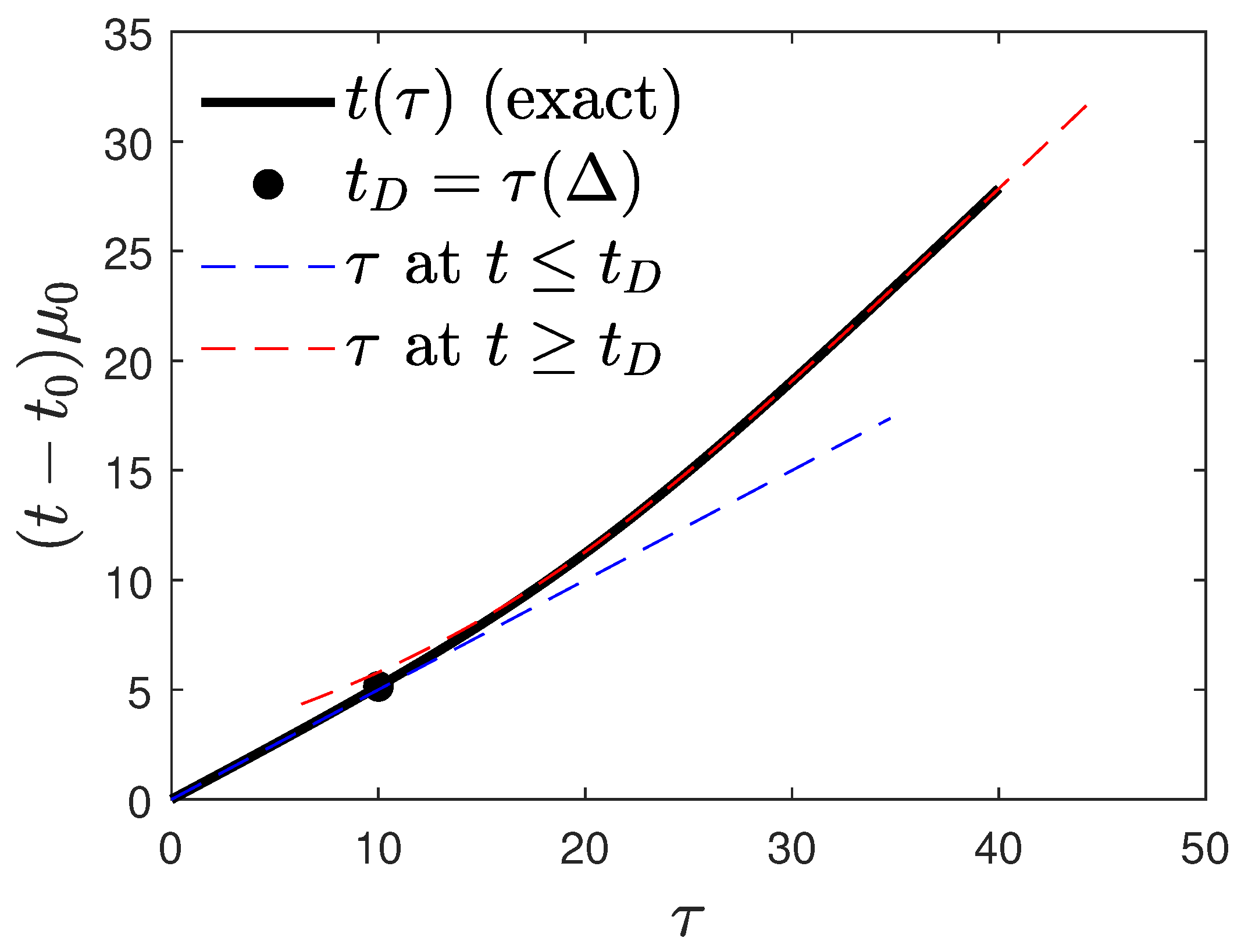
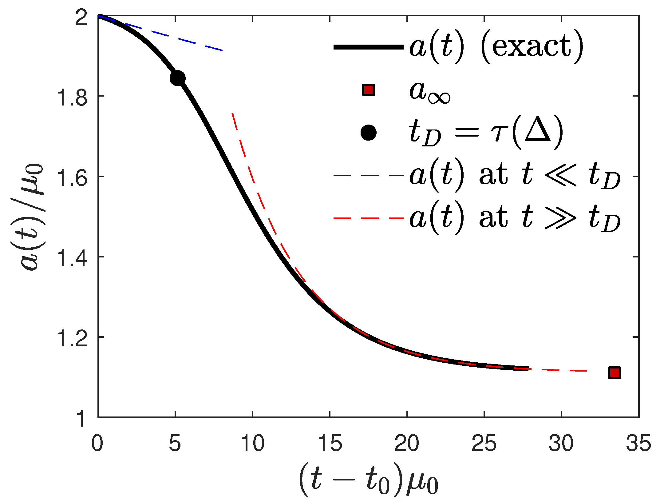
5.2.1. Small Real Times t t D

For small real times t t D , corresponding to reduced times τ Δ , the asymptotics sinh ( τ / Δ ) τ / Δ and cosh ( τ / Δ ) 1 + ( τ 2 / 2 Δ 2 ) are employed to approximate to second order:
ln cosh τ Δ tanh τ c Δ sinh τ Δ ln 1 τ Δ tanh τ c Δ + τ 2 2 Δ 2 τ Δ tanh τ c Δ + 1 tanh 2 ( τ c / Δ ) 2 τ 2 Δ 2 = τ Δ tanh τ c Δ + τ 2 2 Δ 2 cosh 2 τ c / Δ .
In the first step, the smallness of τ / Δ 1 and the approximation ln ( 1 + x ) x x 2 / 2 for small values of x are used, whereas in the second step, the identity 1 tanh 2 ( x ) = cosh 2 ( x ) is employed. In this limit, Equation (29) then yields, with the help of abbreviation (24), the quadratic equation,
τ 2 + 2 k 0 Δ cosh 2 τ c / Δ K τ 2 μ 0 Δ ( t t 0 ) cosh 2 τ c / Δ K .
One can note that K > 0 is positive for values k 1 > k 0 and negative K < 0 in the opposite case, k 1 < k 0 . In the more relevant case of positive K > 0 , Equation (32) is solved by
τ ( t ) k 0 Δ cosh 2 ( τ c / Δ ) K 1 + 2 K μ 0 ( t t 0 ) k 0 2 Δ cosh 2 ( τ c / Δ ) 1 ( t t D ) .
For real times,
t t 0 k 0 2 Δ cosh 2 ( τ c / Δ ) 2 K μ 0 ,
the small time solution (33) approaches the linear relationship
τ ( t t 0 ) μ 0 k 0 .
Differentiating Equation (33) with respect to t then yields for the real-time dependence of the infection rate at small times:
a ( t ) μ 0 k 0 1 + 2 K μ 0 ( t t 0 ) k 0 2 Δ cosh 2 ( τ c / Δ ) ( t t D ) ,
which decreases for positive K from its initial value a 0 = μ 0 / k 0 .

5.2.2. Large Real Times t t D

Likewise for large real times t t D corresponding to τ Δ ,
cosh τ Δ = e τ / Δ 2 1 + e 2 τ / Δ , sinh τ Δ = e τ / Δ 2 1 e 2 τ / Δ ,
are inserted in the way that, in this limit,
ln cosh τ Δ tanh τ c Δ sinh τ Δ = τ Δ ln 2 + ln 1 tanh τ c Δ + ln 1 + 1 + tanh ( τ c / Δ ) 1 tanh ( τ c / Δ ) e 2 τ / Δ τ Δ ln 2 + ln 1 tanh τ c Δ + 1 + tanh ( τ c / Δ ) 1 tanh ( τ c / Δ ) e 2 τ / Δ ,
and, consequently, at late times, Equation (29) can be approximated as
τ + ( k 1 k 0 ) Δ k 1 [ 1 tanh ( τ c / Δ ) ] e 2 τ / Δ μ 0 ( t t 0 ) + K Δ [ ln 2 ln ( 1 tanh ( τ c / Δ ) ) ] k 1 .
At late time τ Δ , the second term on the left-hand side of Equation (39) is much smaller than the first term. One therefore obtains as approximate solution of Equation (30):
τ ( t ) μ 0 ( t t 0 ) + K Δ [ ln 2 ln ( 1 tanh ( τ c / Δ ) ) ] k 1 Δ ( k 1 k 0 ) [ 1 tanh ( τ c / Δ ) ] 2 K / k 1 1 k 1 2 2 K / k 1 exp 2 μ 0 ( t t 0 ) Δ k 1 ( t t D ) ,
and the real time derivative of this equation then provides for the infection rate at late times,
a ( t ) μ 0 k 1 1 + k 1 k 0 k 1 1 tanh ( τ c / Δ ) 2 2 K / k 1 1 exp 2 μ 0 ( t t 0 ) Δ k 1 ( t t D ) ,
which decreases to its final value a = μ 0 / k 1 in the limit t for positive values of K > 0 corresponding to k 1 > k 0 .
Figure 10 and Figure 11 compare the exact real time dependencies t ( τ ) as a function of the reduced time τ and the real time dependence of the infection rate a ( t ) , respectively, with their analytical approximations at small and large real times for the case of a constant recovery rate. The agreement between the exact results and the approximations seems acceptable.

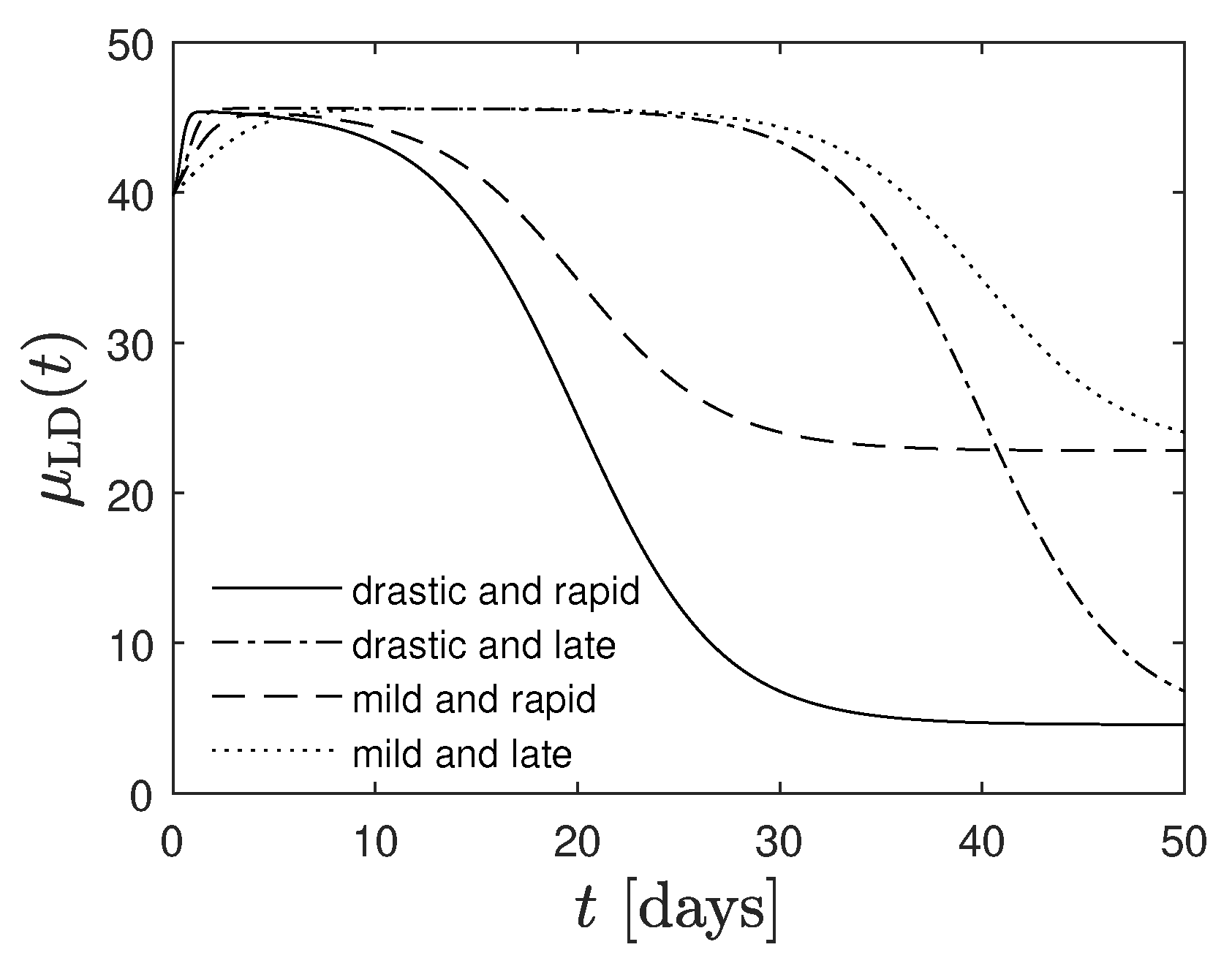
5.2.3. Variable Recovery Rate μ ( t )

Finally, let us note that for a general variable but pre-specified real time dependence of the recovery rate μ ( t ) , Equation (29) reads:
t 0 t d t μ ( t ) = ( k 1 K ) τ + K Δ ln cosh τ Δ tanh τ c Δ sinh τ Δ .
Only if the functional real time dependence μ ( t ) is given, this equation can be analyzed further.

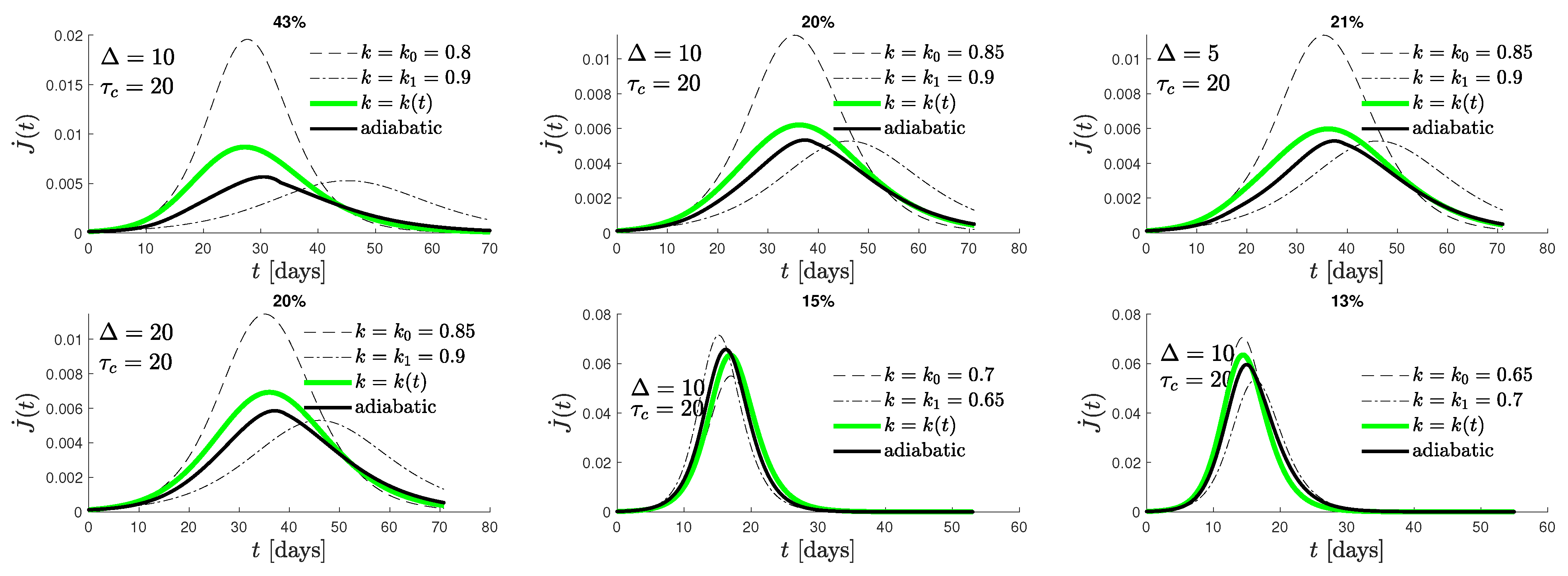
5.3. Real Time Dependence of the Rate of New Infections for a Constant Recovery Rate

The case of a pre-specified constant recovery rate and a real-time-dependent infection rate are regarded as important. In this case, the resulting real-time dependence of the rate of new infections is calculated:
J ˙ ( t ) = a ( t ) j ( τ ( t ) )
using the results for a ( t ) and τ ( t ) from Section 5.2.
Figure 12 shows the adiabatic approximation from version IV in comparison with the exact numerical results and also the limiting KSSIR-variations adopting the initial ratio, k 0 , and final ratio, k 1 , at all times.

6. Summary and Conclusions

The temporal evolution of pandemics described by the susceptible-infectious-recovered (SIR)-compartment model is sensitively determined by the time dependence of the infection ( a ( t ) ) and recovery ( μ ( t ) ) rates. These two rates regulate the transitions from the susceptible to the infected compartment and from the infected to the recovered compartment, respectively. Starting from the pioneering studies [1,2], many numerical solutions of the SIR equations have used stationary values of the two rates, an assumption also made in the analytical solution by Harko et al. [7]. An essential improvement regarding analytical SIR-solutions has been provided by the KSSIR-model developed by us [8,9], holding for arbitrary but given time dependencies of the infection rate a ( t ) for the case of a stationary ratio k = μ ( t ) / a ( t ) , implying that the recovery rate has exactly the same time dependence as the infection rate. This generalization to a time-dependent infection rate is important as such time dependencies are caused by non-pharmaceutical interventions (NPIs) conducted during pandemic outbreaks.
In the current study, apparently for the first time, approximated SIR-solutions are derived for different time dependencies of the infection and recovery rates so that their ratio no longer is constant and becomes also time-dependent. The analysis presented here is based on the adiabatic approximation assuming time-dependent ratios k ( t ) , slowly varying in comparison to the typical time characteristics of the pandemic wave. For such slow variations, the available analytical approximations from the KSSIR-model are used and the adopted time-dependent ratio of the two rates are inserted a posteriori.
Instead of investigating endless different combinations of the time dependencies of the two rates a ( t ) and μ ( t ) , a suitably parameterized reduced-time-dependence of the ratio k ( τ ) is adopted. Along with the definition of the reduced time, this parameterized ratio k ( τ ) allows us to represent a great variety of different time dependencies of the infection and recovery rates. This includes the important case of a stationary recovery rate but a time-dependent infection rate which is investigated in detail.
In each considered case, the obtained solutions from the adiabatic approximation in its four different studied variants are compared to the exact numerical solutions of the SIR-equations. In the worst case, the maximum deviation is 68.1% but in most shown examples much less. This acceptable agreement provides strong confidence in the accuracy of the proposed adiabatic approximation. The adiabatic approximation works best for small differences | k 1 k 0 | between the final ( k 1 ) and initial ( k 0 ) values of the function k ( τ ) ; the maximum deviation for the rate of of new infections scales roughly as 400 | k 1 k 0 | percent.
Analytical solutions are a key to understanding complicated systems. The paper is focused on studying the adequation between the approximation and the true solution, which is essential for this methodology to gain acceptance in epidemiology. The analytical calculations of the SIR model have been shown to enter healthcare decision making [34,35,36,37,38], help in the development of robust and effective pandemic surveillance systems [39], support the investigation of spatial spreading of infections [40,41], provide guidance in the modeling of digital and manual contact tracing [42], allow to forecast the long-term trends of the pandemic evolution [43,44,45], and help to quantify noise from the analytical and numerical point of view [46]. A sensitivity analysis of the presented results in the presence of noise remains beyond the scope of the current study.
The analytical improvements now available will certainly simplify the future public health-care decision-making to cope with aggressive pandemic outbursts. The improvements comprise both, the rather accurate explicit analytical solutions of the SIR-equations and its generalizations such as the SIRV-equations (which includes vaccination denoted by “V”), and the adiabatic approximation for the slowly time-dependent ratios of the infection and recovery rate presented here. The improvements should allow a more robust forecast of the temporal evolution of pandemic outbursts including the effect of taken non-pharmaceutical interventions which will result in predictions regarding the tolerable maximum seven-day incidence value for given health capacities in different countries as well as the estimate of fatality rates and total number of fatalities (for a recent application to the omicron wave, see [11]). Yet even more can be learned on the influence of different non-pharmaceutical interventions on the pandemic evolution: in particular, it should be possible to quantity the parameters of the chosen functional ratio (6) caused by different interventions. However, for such future quantitative studies, a much improved and more complete monitoring of the rate of newly infected persons is necessary. The present data for the omicron mutant are not accurate enough for such studies as the high values for the estimated dark numbers of infections [11] in Great Britain (5.0), Germany (4.4) and Switzerland (2.8) indicate.

Author Contributions

Conceptualization, R.S.; methodology, R.S. and M.K.; software, M.K.; investigation, R.S. and M.K.; writing—original draft preparation, R.S.; writing—review and editing, M.K. All authors have read and agreed to the published version of the manuscript.

Funding

This research received no external funding.

Data Availability Statement

All data required to reproduce the results are part of the present manuscript.

Conflicts of Interest

The authors declare no conflict of interest.

References

  1. Kermack, W.O.; McKendrick, A.G. A contribution to the mathematical theory of epidemics. Proc. R. Soc. A Math. Phys. Eng. Sci. 1927, 115, 700–721. [Google Scholar] [CrossRef] [Green Version]
  2. Kendall, D.G. Deterministic and stochastic epidemics in closed populations. In Proceedings of the Third Berkeley Symposium on Mathematical Statistics and Probability, Los Angeles, CA, USA, December 1954 and July–August 1955; Neyman, J., Ed.; University of California Press: Berkeley, CA, USA; Los Angeles, CA, USA, 1956; Volume 4, pp. 149–165. Available online: https://digitalassets.lib.berkeley.edu/math/ucb/text/math_s3_v4_article-08.pdf (accessed on 25 April 2022).
  3. Hethcode, H.W. The mathematics of infectious deseases. SIAM Rev. 2000, 42, 599. [Google Scholar] [CrossRef] [Green Version]
  4. Keeling, M.J.; Rohani, F. Modeling Infectious Diseases in Humans and Animals; Princeton University Press: Princeton, NJ, USA, 2007. [Google Scholar]
  5. Schlickeiser, R.; Kröger, M. Analytical modelling of the temporal evolution of epidemics outbreaks accounting for vaccinations. Physics 2021, 3, 386–426. [Google Scholar] [CrossRef]
  6. Estrada, E. COVID-19 and SARS-CoV-2. Modeling the present, looking at the future. Phys. Rep. 2020, 869, 1–51. [Google Scholar] [CrossRef]
  7. Harko, T.; Lobo, F.S.N.; Mak, M.K. Exact analytical solution of the susceptible-infected-recovered (SIR) epidemic model and of the SIR model with equal death and birth rates. Appl. Math. Comput. 2014, 236, 184–194. [Google Scholar] [CrossRef] [Green Version]
  8. Kröger, M.; Schlickeiser, R. Analytical solution of the SIR-model for the temporal evolution of epidemics. Part A: Time-independent reproduction factor. J. Phys. A 2020, 53, 505601. [Google Scholar] [CrossRef]
  9. Schlickeiser, R.; Kröger, M. Analytical solution of the SIR-model for the temporal evolution of epidemics: Part B. Semi-time case. J. Phys. A 2021, 54, 175601. [Google Scholar] [CrossRef]
  10. Kröger, M.; Schlickeiser, R. Verification of the accuracy of the SIR model in forecasting based on the improved SIR model with a constant ratio of recovery to infection rate by comparing with monitored second wave data. R. Soc. Open Sci. 2021, 8, 211379. [Google Scholar] [CrossRef]
  11. Schlickeiser, R.; Kröger, M. Forecast of omicron wave time evolution. COVID 2022, 2, 216–229. [Google Scholar] [CrossRef]
  12. Lerche, I. Epidemic evolution: Multiple analytical solutions for the SIR model. Preprints 2020, 2020080479. [Google Scholar] [CrossRef]
  13. Schoner, G.; Haken, H. A systematic elimination procedure for Ito stochastic differential-equations and the adiabatic approximation. Z. Physik B 1987, 68, 89–103. [Google Scholar] [CrossRef]
  14. Yukalov, V.I. Adiabatic theorems for linear and nonlinear Hamiltonians. Phys. Rev. A 2009, 79, 052117. [Google Scholar] [CrossRef] [Green Version]
  15. Wentzel, G. Eine Verallgemeinerung der Quantenbedingungen für die Zwecke der Wellenmechanik. Z. Physik 1926, 38, 518–529. [Google Scholar] [CrossRef]
  16. Kramers, H.A. Wellenmechanik und halbzahlige Quantisierung. Z. Physik 1926, 39, 828–840. [Google Scholar] [CrossRef]
  17. Brillouin, L. La mécanique ondulatoire de Schrödinger: Une méthode générale de résolution par approximations successives. Compt. Rend. Hebd. Séances Acad. Sci. 1926, 183, 24–26. Available online: http://gallica.bnf.fr/ark:/12148/bpt6k3136h/f24 (accessed on 25 April 2022).
  18. Jeffreys, H. On certain approximate solutions of linear differential equations of the second order. Proc. Lond. Math. Soc. 1925, 23, 428–436. [Google Scholar] [CrossRef]
  19. Born, M.; Oppenheimer, R. Zur Quantentheorie der Molekeln. Ann. Phys. 1927, 389, 457–484. [Google Scholar] [CrossRef]
  20. Schüttler, J.; Schlickeiser, R.; Schlickeiser, J.; Kröger, M. COVID-19 predictions using a Gauss model, based on data from april 2. Physics 2020, 2, 197–212. [Google Scholar] [CrossRef]
  21. Fricke, L.M.; Glockner, S.; Dreier, M.; Lange, B. Impact of non-pharmaceutical interventions targeted at COVID-19 pandemic on influenza burden—A systematic review. J. Infect. 2021, 82, 1–35. [Google Scholar] [CrossRef]
  22. Kasting, M.L.; Head, K.J.; Hartsock, J.A.; Sturm, L.; Zimet, G.D. Public perceptions of the effectiveness of recommended non-pharmaceutical intervention behaviors to mitigate the spread of SARS-CoV-2. PLoS ONE 2020, 15, e0241662. [Google Scholar] [CrossRef]
  23. Ullah, S.; Khan, M.A. Modeling the impact of non-pharmaceutical interventions on the dynamics of novel coronavirus with optimal control analysis with a case study. Chaos Solitons Fractals 2020, 139, 110075. [Google Scholar] [CrossRef] [PubMed]
  24. Flaxman, S.; Mishra, S.; Gandy, A.; Unwin, H.J.T.; Mellan, T.A.; Coupland, H.; Whittaker, C.; Zhu, H.; Berah, T.; Eaton, J.W.; et al. Estimating the effects of non-pharmaceutical interventions on COVID-19 in Europe. Nature 2020, 584, 257–261. [Google Scholar] [CrossRef] [PubMed]
  25. Hsiang, S.; Allen, D.; Annan-Phan, S.; Bell, K.; Bolliger, I.; Chong, T.; Druckenmiller, H.; Huang, L.Y.; Hultgren, A.; Krasovich, E.; et al. The effect of large-scale anti-contagion policies on the COVID-19 pandemic. Nature 2020, 584, 262–267. [Google Scholar] [CrossRef] [PubMed]
  26. Nicola, M.; O’Neill, N.; Sohrabi, C.; Khan, M.; Agha, M.; Agha, R. Evidence based management guideline for the COVID-19 pandemic—Review article. Int. J. Surg. 2020, 77, 206–216. [Google Scholar] [CrossRef] [PubMed]
  27. Eikenberry, S.E.; Mancuso, M.; Iboi, E.; Phan, T.; Eikenberry, K.; Kuang, Y.; Kostelich, E.; Gumel, A.B. To mask or not to mask: Modeling the potential for face mask use by the general public to curtail the COVID-19 pandemic. Infect. Dis. Model. 2020, 5, 293–308. [Google Scholar] [CrossRef] [PubMed]
  28. Merler, S.; Ajelli, M.; Fumanelli, L.; Gomes, M.F.C.; Pastore y Piontti, A.; Rossi, L.; Chao, D.L.; Longini, I.M., Jr.; Halloran, M.E.; Vespignani, A. Spatiotemporal spread of the 2014 outbreak of Ebola virus disease in Liberia and the effectiveness of non-pharmaceutical interventions: A computational modelling analysis. Lancet Infect. Dis. 2015, 15, 204–211. [Google Scholar] [CrossRef] [Green Version]
  29. Ferguson, N.M.; Cummings, D.A.T.; Fraser, C.; Cajka, J.C.; Cooley, P.C.; Burke, D.S. Strategies for mitigating an influenza pandemic. Nature 2006, 442, 448–452. [Google Scholar] [CrossRef]
  30. Haas, F.; Kröger, M.; Schlickeiser, R. Multi-hamiltonian structure of the epidemics model accounting for vaccinations and a suitable test for the accuracy of its numerical solvers. J. Phys. A 2022. [Google Scholar] [CrossRef]
  31. Shampine, L.F.; Hosea, M.E. Analysis and implementation of TR-BDF2. Appl. Numer. Math. 1996, 20, 21–37. [Google Scholar]
  32. Shampine, L.F.; Reichelt, M.W.; Kierzenka, J.A. Solving index-1 DAEs in matlab and simulink. SIAM Rev. 1999, 41, 538–552. [Google Scholar] [CrossRef]
  33. Schlickeiser, R.; Kröger, M. Epidemics forecast from SIR-modeling, verification and calculated effects of lockdown and lifting of interventions. Front. Phys. 2021, 8, 593421. [Google Scholar] [CrossRef]
  34. Mechanic, D. Approaches for coordinating primary and specialty care for persons with mental illness. Gen. Hosp. Psych. 1997, 19, 395–402. [Google Scholar] [CrossRef]
  35. Yuan, E.C.; Alderson, D.L.; Stromberg, S.; Carlson, J.M. Optimal Vaccination in a stochastic epidemic model of two non-interacting populations. PLoS ONE 2015, 10, e0115826. [Google Scholar] [CrossRef] [Green Version]
  36. Hu, Y.; Zhong, W.; Cen, Y.; Han, S.; Feng, Z.; Zhang, X.; Li, W.; Wang, L.; Li, B.; Issa, S.; et al. Prediction of epidemiological characteristics of vascular cognitive impairment using SIR mathematical model and effect of brain rehabilitation and health measurement system on cognitive function of patients. Res. Phys. 2021, 25, 104331. [Google Scholar] [CrossRef]
  37. Fiscon, G.; Salvadore, F.; Guarrasi, V.; Garbuglia, A.R.; Paci, P. Assessing the impact of data-driven limitations on tracing and forecasting the outbreak dynamics of COVID-19. Comput. Biol. Med. 2021, 135, 104657. [Google Scholar] [CrossRef]
  38. d’Andrea, V.; Gallotti, R.; Castaldo, N.; De Domenico, M. Individual risk perception and empirical social structures shape the dynamics of infectious disease outbreaks. PLoS Comput. Biol. 2022, 18, e1009760. [Google Scholar] [CrossRef]
  39. Jiang, J.Y.; Zhou, Y.; Chen, X.; Jhou, Y.R.; Zhao, L.; Liu, S.; Yang, P.C.; Ahmar, J.; Wang, W. COVID-19 surveiller: Toward a robust and effective pandemic surveillance system basedon social media mining. Philos. Trans. R. Soc. A 2022, 380, 20210125. [Google Scholar] [CrossRef] [PubMed]
  40. Roman, H.E.; Croccolo, F. Spreading of infections on network models: Percolation clusters and random trees. Mathematics 2021, 9, 3054. [Google Scholar] [CrossRef]
  41. Baerwolff, G. A local and time resolution of the COVID-19 propagation—A two-dimensional approach for Germany including diffusion phenomena to describe the spatial spread of the COVID-19 pandemic. Physics 2021, 3, 536–548. [Google Scholar] [CrossRef]
  42. Rusu, A.C.; Emonet, R.; Farrahi, K. Modelling digital and manual contact tracing for COVID-19. Are low uptakes and missed contacts deal-breakers? PLoS ONE 2021, 16, e0259969. [Google Scholar] [CrossRef]
  43. Kartono, A.; Karimah, S.V.; Wahyudi, S.T.; Setiawan, A.A.; Sofian, I. Forecasting the long-term trends of coronavirus disease 2019 (COVID-19) epidemic using the susceptible-infectious-recovered (SIR) model. Infect. Disease Rep. 2021, 13, 668–684. [Google Scholar] [CrossRef] [PubMed]
  44. Hynd, R.; Ikpe, D.; Pendleton, T. Two critical times for the SIR model. J. Math. Anal. Appl. 2022, 505, 125507. [Google Scholar] [CrossRef]
  45. Kavitha, C.; Gowrisankar, A.; Banerjee, S. The second and third waves in India: When will the pandemic be culminated? Eur. Phys. J. Plus 2021, 136, 596. [Google Scholar] [CrossRef] [PubMed]
  46. Hussain, S.; Madi, E.N.; Khan, H.; Etemad, S.; Rezapour, S.; Sitthiwirattham, T.; Patanarapeelert, N. Investigation of the stochastic modeling of COVID-19 with environmental noise from the analytical and numerical point of view. Mathematics 2021, 9, 3122. [Google Scholar] [CrossRef]
Figure 1. The ratio k ( τ ) (6) as a function of the reduced time τ (3) for the initial and final values k 0 = 0.8 and k 1 = 0.9 , respectively, for different choices of the parameters τ c and Δ .
Physics 04 00034 g001
Figure 2. Results for versions I–IV of KSSIR model [8,9] with the dimensionless parameters of the ratio (6) as indicated in the most left panel, and η = 10 4 . The second, third, fourth and fifth (left to right) panels display the calculated dependence of the fractions of susceptible, S ( τ ) , infected, I ( τ ) , and recovered/removed, R ( τ ) , persons, and the rate of new infections, j ( τ ) (16), respectively, as a function of the reduced (dimensionless) time, τ . The green curve provides the exact numerical result, the solid black curve shows the adiabatic approximation, the dashed curve shows the KSSIR-variation adopting the initial ratio, k 0 , at all times, and the dot-dashed curve displays the KSSIR-variation adopting the final ratio, k 1 , at all times. The percentages on top of each panel indicate the maximum relative deviations between exact and approximate solutions. See text for details.
Physics 04 00034 g002
Figure 3. Same as Figure 2 but with another set of the parameters ( k 0 = 0.85 , k 1 = 0.9 , Δ = 10 , and τ c = 20 ) of the ratio k ( τ ) (6).
Physics 04 00034 g003
Figure 4. Same as Figure 2 but with another set of the parameters ( k 0 = 0.85 , k 1 = 0.9 , Δ = 5 , and τ c = 20 ) of the ratio k ( τ ) (6).
Physics 04 00034 g004
Figure 5. Same as Figure 2 but with another set of the parameters ( k 0 = 0.85 , k 1 = 0.9 , Δ = 20 , and τ c = 20 ) of the ratio k ( τ ) (6).
Physics 04 00034 g005
Figure 6. Same as Figure 2 but with another set of the parameters ( k 0 = 0.7 , k 1 = 0.65 , Δ = 10 , and τ c = 20 ) of the ratio k ( τ ) (6). Here, a decreasing ratio with reduced time is chosen in contrast to Figure 2, Figure 3, Figure 4 and Figure 5, Figure 7 and Figure 8, where increasing ratios are considered.
Physics 04 00034 g006
Figure 7. Same as Figure 2 but with another set of the parameters ( k 0 = 0.65 , k 1 = 0.7 , Δ = 10 , and τ c = 20 ) of the ratio k ( τ ) (6).
Physics 04 00034 g007
Figure 8. Same as Figure 2 but with another set of the parameters ( k 0 = 0.7 , k 1 = 0.9 , Δ = 10 , and τ c = 20 ) of the ratio k ( τ ) (6).
Physics 04 00034 g008
Figure 9. The lockdown recovery rate, μ LD ( t ) (21), in the case of pre-specified lockdown infection rate, a LD (19), using k 0 = 0.7 , k 1 = 0.8 , a 0 = 57 days 1 , t b = 7 days, τ c = a 0 t a , Δ = 10 q t a for the four cases: drastic ( q = 0.1 ) and rapid ( t a = 20 days); drastic ( q = 0.1 ) and late ( t a = 40 days); mild ( q = 0.5 ) and rapid ( t a = 20 days); and mild ( q = 0.5 ) and late ( t a = 40 days), as indicated.
Physics 04 00034 g009
Figure 10. Real time, t ( τ ) , versus τ (solid black line) for the case of k 0 = 0.5 , k 1 = 0.9 , τ c = 20 , Δ = 10 at fixed constant infection rate μ 0 . The dot indicates the value at the transition time, t D (30), and the asymptotic expressions (35) and (40) for small and large times, respectively, are shown by dashed lines of different colors as indicated.
Physics 04 00034 g010
Figure 11. Infection rate, a ( t ) , versus real time t (solid black line) for the parameters used in Figure 10. The dot indicates the value at the transition time, t D (30), the red square shows a = μ 0 / k 1 at t , while the asymptotic expressions (36) and (41) for small and large times, respectively, are shown by dashed lines of different colors as indicated.
Physics 04 00034 g011
Figure 12. Daily new rate of infected persons, J ˙ ( t ) (43), versus real time t in the case of a constant recovery rate for the parameters from Figure 2, Figure 3, Figure 4, Figure 5, Figure 6, Figure 7 and Figure 8. The adiabatic version IV (solid black line) is compared with the exact numerical solution (green) and the reference cases of constant k ( t ) = k 0 (dashed) and k ( t ) = k 1 (dash-dotted).
Physics 04 00034 g012
Publisher’s Note: MDPI stays neutral with regard to jurisdictional claims in published maps and institutional affiliations.

