The Nuclear Shell Model towards the Drip Lines


Department of Physics and Astronomy, and the Facility for Rare Isotope Beams, Michigan State University, East Lansing, MI 48824-1321, USA
Physics 2022, 4(2), 525-547; https://doi.org/10.3390/physics4020035
Submission received: 7 March 2022
/
Revised: 13 April 2022
/
Accepted: 14 April 2022
/
Published: 12 May 2022
(This article belongs to the Special Issue The Nuclear Shell Model 70 Years after Its Advent: Achievements and Prospects)
Abstract
:Applications of configuration-mixing methods for nuclei near the proton and neutron drip lines are discussed. A short review of magic numbers is presented. Prospects for advances in the regions of four new “outposts” are highlighted: O, Si, Ca and Ni. Topics include shell gaps, single-particle properties, islands of inversion, collectivity, neutron decay, neutron halos, two-proton decay, effective charge, and quenching in knockout reactions.
1. Introduction
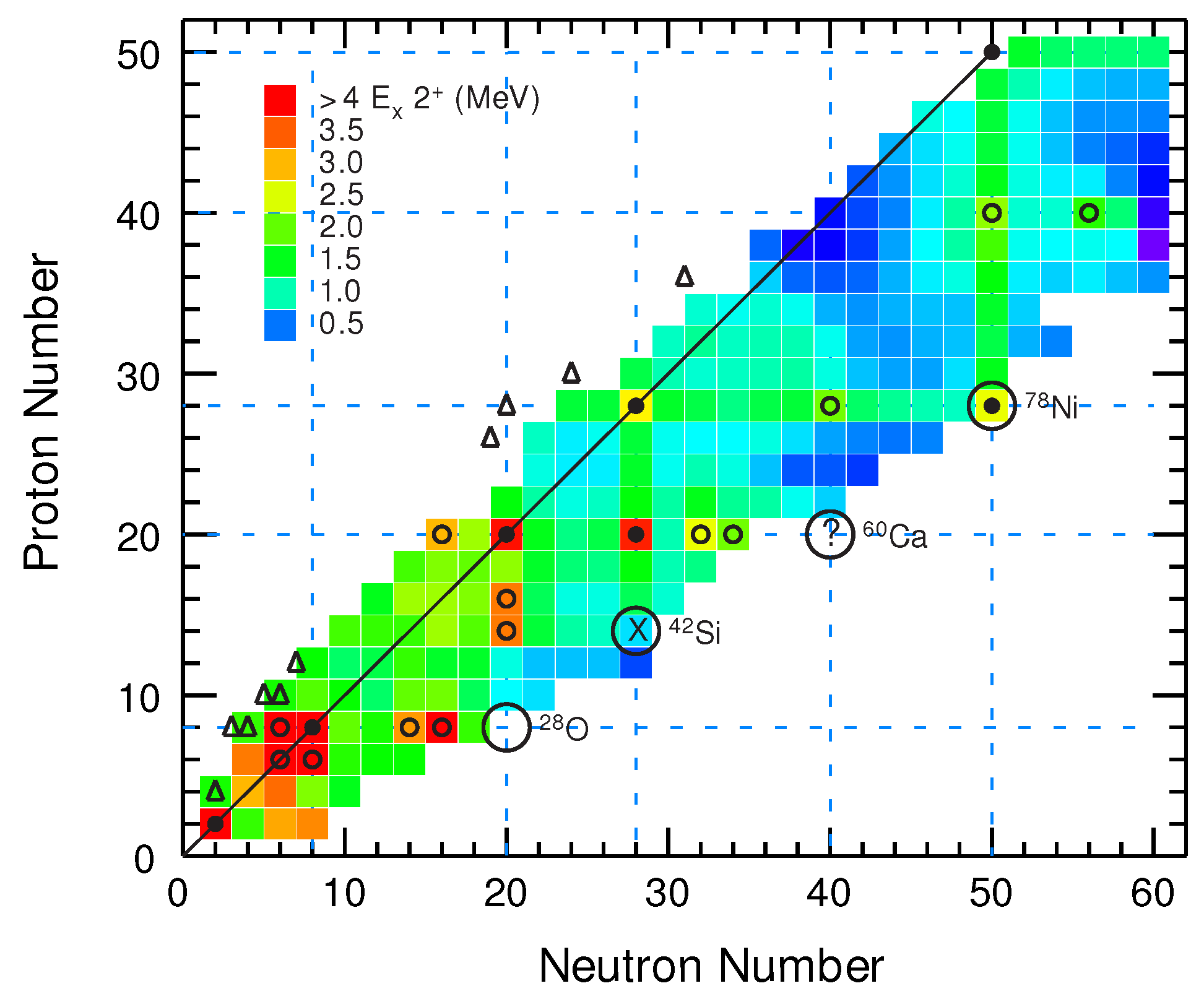
The starting point for the nuclear shell model is the establishment of model spaces that allow for tractable configuration-interaction (CI) calculations from which we are able to understand and predict the properties of low-lying states [1,2,3,4,5]. This choice is based on the observation that a few even–even nuclei can be interpreted in terms of having magic numbers for Z (atomic number) or N (nucleon number) and doubly-magic numbers for a given . These magic numbers can be inferred from experimental excitation energies of 2 states shown for the low end of the nuclear chart in Figure 1. Magic numbers are those values of Z or N for nuclei that have a relatively high 2 energy within a series of isotopes or isotones.
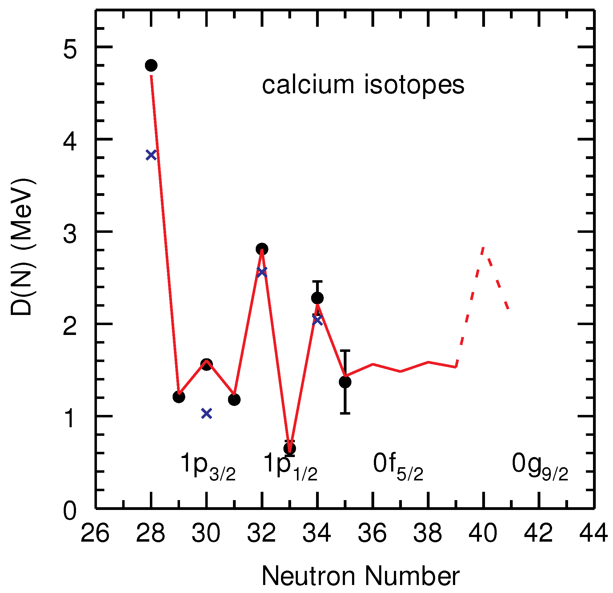
Another measure of magic numbers is given by the double difference in the binding energy, BE, defined by
for isotopes ( with Z held fixed) or isotones ( with N held fixed) can also be used to measure shell gaps [6]. An example for the neutron-rich calcium isotopes is shown in Figure 2 (the dashed line extrapolation to is discussed below.) The value of at these magic numbers gives the effective shell gap. In between the magic numbers, gives the pairing energy [6]. The excitation energies of the 2 states at , 32 and 34, also shown in Figure 2, are close to the values at these magic numbers. The neutron gaps at and 34 are weaker than the gap at , but they are strong enough to allow the configurations to be dominated by the orbitals, shown in Figure 2.
In the simplest model, the magic number is associated with a ground state that has a closed-shell configuration for the given value of Z or N. The following is from footnote 9 in [7]. It was Eugene Paul Wigner who coined the term “magic number”. Steven A. Moszkowski, who was a student of Maria Goeppert-Mayer, in a talk presented at the American Physical Society meeting in Indianapolis, 4 May 1996 said: “Wigner believed in the liquid drop model, but he recognized, from the work of Maria Mayer, the very strong evidence for the closed shells. It seemed a little like magic to him, and that is how the words ‘Magic Numbers’ were coined”. The discovery of “magic numbers” lead M. Goeppert-Mayer, and independently J. Hans D. Jensen in Germany, one year later, in 1949, to the construction of the shell model with strong spin–orbit coupling, and to the Nobel Prize they shared with Wigner in 1963.
The nuclei marked with closed circles in Figure 1 are commonly used to define the boundaries of CI model spaces. Those indicated by small open circles are usually contained within a larger CI model spaces. Historically, the size of the assumed model space has depended on the computational capabilities. At the very beginning in the 1960s, they were the model space bounded by He and O, and the model space bounded by Ca and Ni.
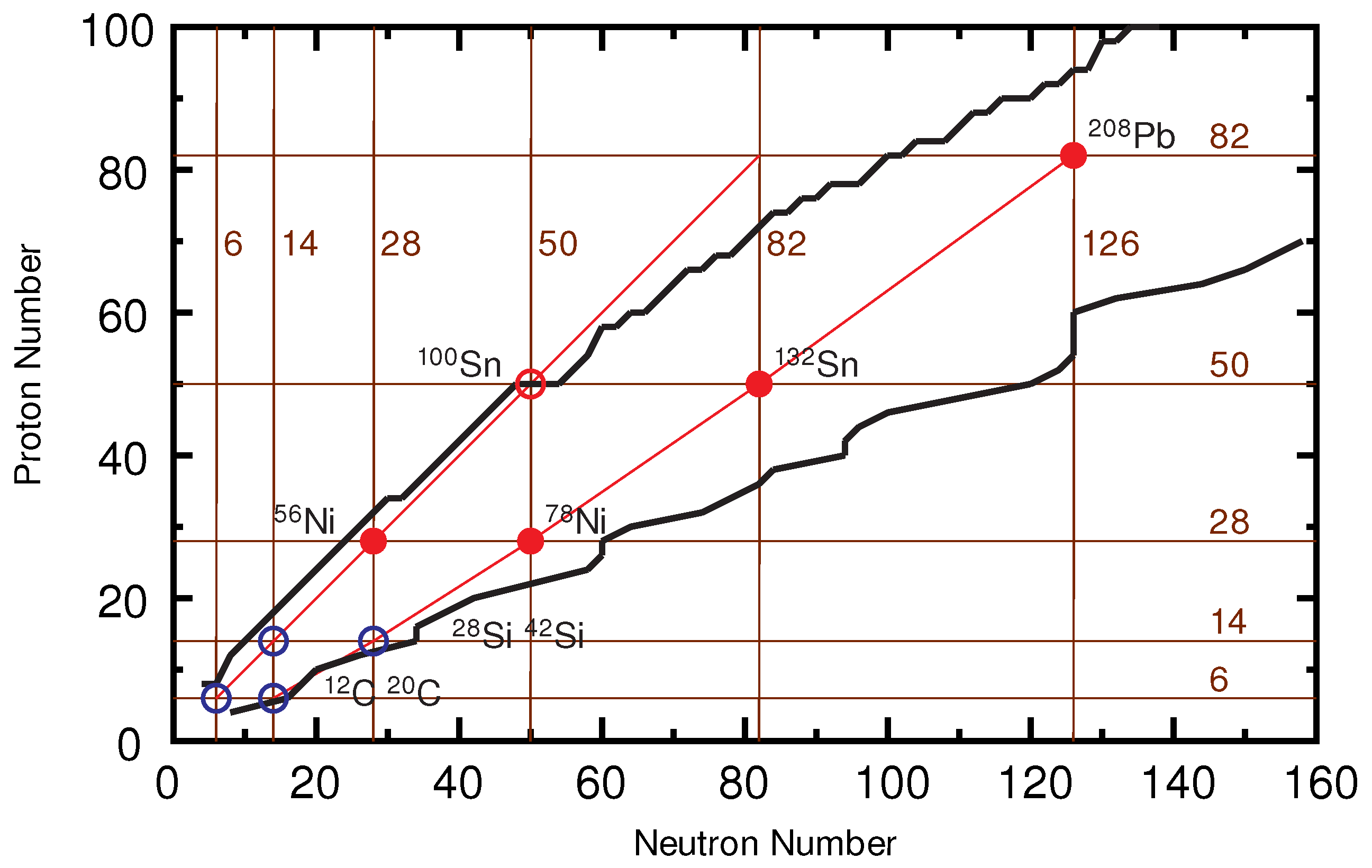
For heavy nuclei, doubly-magic nuclei are associated with the shell gaps at 28, 50, 82 and 126. These gaps are created by the spin–orbit splitting of the high ℓ orbitals, which lowers the the single-particle energies for ℓ = 3 (28), ℓ = 4 (50), ℓ = 5 (82) and ℓ = 6 (126). Since the two j values for a given high ℓ value are split, 28, 50, 82 and 126 will be referred to as magic numbers. The nuclei with magic numbers for both protons and neutrons will be called double- closed-shell nuclei. These are shown by the red circles in Figure 3: Pb, Sn, Sn, Ni and Ni. The open red circle for Sn indicates that it is expected to be double- magic [14], but it has not yet been confirmed experimentally. The continuation of the double- sequence with ℓ = 2 (14) and ℓ = 1 (6) is shown by the open blue circles for Si, Si, C and C on the lower left-hand side of Figure 3. As discussed below, the calculations for these nuclei show rotational bands with positive quadrupole moments indicative of an oblate intrinsic shape.
In light nuclei, magic numbers 2, 8, 20 and 40 are associated with the filling of a major harmonic-oscillator shell with ( is the radial quantum number), where both members of the spin–orbit pair are filled. Since one can recouple the two orbitals with the same ℓ value to total angular momentum L and total spin S, 2, 8, 20 and 40 will be referred to as magic numbers.
The magic numbers for isotopes and isotones are shown by the thin brown lines in Figure 4. There are only three known double- magic nuclei, He, O and Ca shown by the filled red circles in Figure 4. The next one in the sequence would be Zr, but in this case the gap is too small due to the lowering of the single-particle energy from the spin–orbit splitting. As will be discussed below, Ca (the red open circle with a question mark) could be a “fourth” double- magic nucleus. There are regions where the magic numbers for isotopes or isotones dissappear as shown by the blue lines in Figure 4. These will be referred to as “islands of inversion” [15].
The nuclei with green circles in Figure 4 also have doubly-magic properties. The pattern is that when one type of nucleon (proton or neutron) has an magic number, then the other one has a magic number for the filling of each j orbital. These are 6 (), 8 (), 14 (), 16 (), 20 (), 28 (), 32 (), 34 (), 40 (), 50 () and 56 ().
The only addition to the and closed-shell systematics discussed above is for Sr shown in Figure 4, where there is an energy gap between the proton and , states. In early calculations, Sr was used as the closed shell for the model space [16], but more recently the four-orbit model space of ,,, has been used for the isotones [17,18].
For a given shell gap, the magic numbers are more robust than those for . The reason is that deformation for magic numbers starts with a one-particle one-hole (–) excitation of a nucleon in the orbital to the other members of the same oscillator shell, . Since – excitations across closed shell gaps change parity, ground-state deformation for magic numbers must come from – () excitations across the closed shells as in the region of Mg [15].
Let us discuss here results, obtained with Hamiltonians. based on data-driven improvements to the two-body matrix elements, provided by ab initio methods. The ab initio methods are based on two-nucleon (NN) and three-nucleon (NNN) interactions obtained by model-dependent fits to nucleon-nucleon phase shifts and properties of nuclei with to 4. For a given model space, these are renormalized for short-range correlations and for the truncations into the chosen model space to provide a set of two-body matrix elements (TBME) for nuclei near a chosen doubly-closed shell. From this starting point, one attempts to make minimal changes to the Hamiltonian to improve the agreement with energy data for a selected set of nuclei and states within the model space. A convenient way to do this is by using singular value decomposition (SVD) [19]. In many cases, one adjusts specific TBME or combinations of TBME. The most important are the monopole, pairing and quadrupole components. An important part of the universal Hamiltonian is in the evolution of the effective single-particle energies (ESPE) as one changes the number of protons and neutrons. Starting with a closed shell with a given set of single-particle energies, the ESPE as a function of Z and N are determined by the monopole average parts of the TBME [5].
These methods provide “universal” Hamiltonians in the sense that a single set of single-particle energies and two-body matrix elements are applied to all nuclei in the model space, perhaps allowing for some smooth mass dependence. This has turned out to be a practical and useful approximation. As the ab initio, starting points are improved, these “universal” Hamiltonians were replaced by Hamiltonians for a more restricted set of nuclei, or even for individual nuclei as has been done in the valence-space in-medium similarity renormalization group (VS-IMSRG) method [4,20].
The empirical modifications to the effective Hamiltonian account for deficiencies in the more ab initio methods. Most ab initio calculations are carried out in a harmonic-oscillator basis due to its convenient analytical properties. Near the neutron drip lines, the radial wavefunctions become more extended, the single-particle energy spectrum becomes more compressed, and the continuum becomes explicitly more important. To take this into account, the ab initio methods require a very large harmonic-oscillator basis.
Due to the continuum, nuclei near the neutron drip line present a substantial theoretical challenge [2,21]. Methods have been developed that take the continuum into account explicitly. The density matrix renormalization group (DMRG) method [22,23] makes use of a single-particle potential together with a simplified interaction based on halo effective field theory [24,25]. In the Gamow shell model (GSM) [26,27,28], the many-body basis is constructed from a single-particle Berggren ensemble [29,30]. The DMRG and GSM methods rely on use of simplified two-body interactions with adjustable parameters. There is also the shell model embedded in the continuum formalism that can make use of the universal interactions [31]. Recent progress in the GSM method is presented in [32].
Ground-state nuclear halos are a unique feature of nuclei near the neutron drip line [33]. This is due to the loose binding of low-ℓ orbitals with extended radial wavefunctions. The most famous case is that for Li which was observed to have a rapid rise in the nuclear matter radius compared to the trends up to Li [34]. The wavefunction of Li is dominated by a pair of neutrons in the orbital. As discussed below, halos in the region of Ne and Si are dominated by the orbital. Proton halos are not so extreme due to the Coulomb barrier. The excited 1/2 () state of F is a good example of an excited-state halo as determined indirectly from its large Thomas–Ehrman energy shift of 0.87 MeV O to 0.49 MeV in F.
States above the (proton/neutron) separation energy have (proton/neutron) decay widths. In the conventional CI approach, one calculates states whose energy is taken to be the centroid energy of the decaying state. The decay width is calculated using the approximation , where CS is the spectroscopic factor and is the single-particle neutron decay width calculated with a a decay energy, Q, value taken from the shell-model centroid or the experimental centroid if known. The explicit addition of the continuum shifts down the energy relative to its CI energy [31]. Further, the continuum (finite-well potential) is responsible for the Thomas–Ehrman shift for states in proton-rich nuclei compared to those in the neutron-rich mirror nuclei [19].
In this review, I concentrate on four regions of neutron-rich “outposts” whose understanding are most important for future developments. These are shown in Figure 1: O, Si, Ca and Ni. Si is labeled by “×” since it does not have a magic number for protons or neutrons. Ni is labeled by a filled circle since it is now known to be doubly magic [35]. Ca is known to be inside the neutron drip line [36], but its mass and excited states have not yet been measured.
Nuclei that are observed to decay by two protons are shown by the triangles in Figure 1. The two-proton ground-state decays for Fe, Ni, Zn and Kr have half-lives on the order of ms and compete with the decay of those nuclei. An experimental and theoretical summary of the results for those nuclei together with that of Mg has been given in [37]. There is qualitative agreement between experiment and theory. In order to become more quantitative, the experimental errors in the partial half-lives need to be improved. Theoretical models need to be improved to incorporate three-body decay dynamics (presently based on single-orbit configurations) with the many-body CI calculations for the two-nucleon decay amplitudes. The correlations for two-nucleon transfer amplitudes via (t,p) or (He,n) are largely determined by the structure of the triton or He, whereas two-nucleon decay is determined by the decay through the Coulomb and angular-momentum barriers that are dominated by the low-ℓ components. For the lightest nuclei, multi-proton emissions (shown in Figure 1 of [38]) are observed as broad resonances.
Knockout reactions are used to produce nuclei further from stability. The cross sections for these reactions can be compared to theoretical models in terms of the cross-section ratio see [39] for a recent summary. It is observed for nuclei far from stability where is large ( is the one nucleon separation energy) that is near unity when the knocked out nucleon is loosely bound but drops to approximately 0.3 for deeply bound nucleons. This has been attributed to the short- and long-ranged correlations that depletes the occupation of deeply-bound states [40]. The short-ranged correlations are connected to the high-momemtum tail observed in observed in high-energy electron scattering experiments [41]. The long-ranged correlations come fron particle-core coupling and pairing correlations beyond that included within the valence space. Another reason may be the approximations made in the sudden approximation for the dynamics used for the reaction [39]. In the analysis of [40], the factor for loosely-bound nucleons that comes mainly from the long-ranged correlations is expected to be 0.6–0.7 rather than unity. The analysis of experiments [42] find values that depend less on the proton separation energy going from 0.6 to 0.7.
The depends on the CI calculations for the spectroscopic factors. An approximation that is made in CI calculations is that only the change in configurations for the knocked out nucleon contributes to the spectroscopic factor. The radial wavefunctions for all other nucleons in the parent and daughter nuclei are assumed to be the same. However, consider, as an example, the knockout of a deeply bound proton from Ne to F. The size of the neutrons orbtials in Ne and F are changing due to the proximity to the continuum, and the overlap of the spectator neutrons in the nuclei with the atomic mass numbers A and will be reduced from unity. This effect should be contained in ab initio and continuum models [43,44], but an understanding within these models requires an explicit separation of the one-nucleon removal overlaps in terms of the removed nucleon within the basis states for and the radial overlaps between the nuclei with A and .
2. The Region of O
The oxygen isotopes provided the first complete testing ground for theory and experiment from the proton drip line to the neutron drip line [45]. The prediction by the “universal” -shell (USD) Hamiltonian [1,46], in the 1980s that O was a doubly-magic nucleus was later confirmed experimentally in 2009 [47,48,49].
For the one-neutron decay of O, the USD charge-dependent (USDC) Hamiltonian in the shell [19] gives MeV, to be compared to the experimental value of MeV [50]. The explicit addition of the continuum will lower the calculated energy [31]. The calculated value of the spectroscopic factor is (the error, shown in the parentheses for the value last decimal, comes from the comparison of the four -shell Hamiltonians developed in [19]). For the calculated decay width, one obtains keV. keV is obtained using the experimental Q value and a Woods–Saxon potential. The experimental neutron decay width is keV [50]. The theoretical error in the width is probably dominated by the uncertainty in the parameters of the Woods–Saxon potential.
The measured masses of the Na isotopes [51] found more binding near than could be accounted for by the pure configurations; here, the notation is used where n is the number of neutrons excited from to . Hartree–Fock calculations [52] showed that these mass anomalies were associated with a large prolate deformation, where the 2 [N,n,] = 1 [3,3,0] and 3 [3,2,1] Nilsson orbitals from the shell cross the 1 [2,0,0] and 3 [2,0,2] orbitals from the shell near a value for the deformation paramater of = +0.3. The anomaly was confirmed by , CI calculations in [53,54], where in [53] it was called the “collapse of the conventional shell-model”. CI calculations that included components [15,55] showed that nuclei in this region have ground-state wavefunctions dominated by the = 2 component. This is due to a weakened shell gap at below , pairing correlations in the = 2 configurations, and proton–neutron quadrupole correlations that give rise to the Nilsson orbital inversion. In [15], the region of nuclei below Si involved in this inversion was called the “island-of-inversion”.
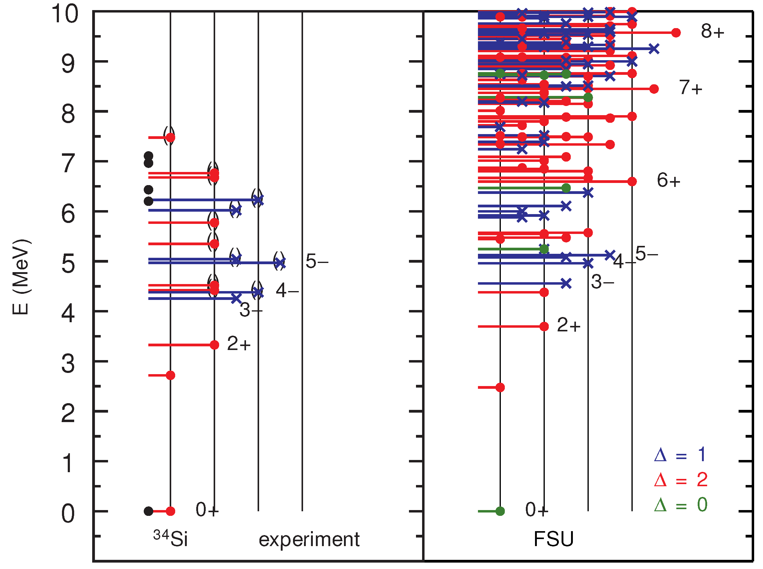
The Hamiltonian, used in [15], was appropriate for pure configurations. This Hamiltonian was modified to account for more recent data related to the energies of and configurations resulting in the new Florida State University (FSU) Hamiltonian [56]. As examples of the type of predictions, results, obtained with the FSU Hamiltonian, are shown for Si in Figure 5, Mg in Figure 6, and F in Figure 7. All of these calculaitons were carried out with NuShellX [57] code and allowed only for neutron excitations from – to –. Calculations in a full basis (ℏ being the reduced Planck constant) with also require the addition of proton excitations from to – and proton exicitations from – to –. In full basis, the 1 spurious states can be removed with the Gloeckner-Lawson method [58]. Comparison to calculations in the full basis with the Oxbash code [59] show that the energies are lowered relative to the basis by up to approximately 200 keV. This shows the , 2 proton and proton–neutron components are small compared to the , 2 neutron components for the low-lying states in these neutron-rich nuclei. For nuclei with , removal of the spurious states in the basis is important.
The barrier between the (spherical) and (deformed) configurations reduces the mixing between the lowest energy states of each configuration. When one combines the and configurations in CI calculations, the state that is dominated by is pushed down in energy by the mixing with many configurations mainly due to the increase in the pairing energy. If one were to start with the FSU Hamiltonian and add off-diagonal TBME of the type , the components dominated by = 0 would be pushed down in energy due to this increase in pairing. However, this results in a double-counting since the part FSU interaction is already implicitly renormalized for the admixtures. In addition, to achieve convergence in the mixed wavefunctions, one has to add = 4 and higher. This results in large matrix dimensions.
When one mixes the components, one has to modify parts of the Hamiltonian that are diagonal in . This is sometimes performed by changing the pairing strength in the , two-body matrix elements, so that the ground-state binding energies agree with experimental values. Hamiltonians that have been designed for mixed configurations are called SDPF-U-MIX [60] and SDPF-M [61,62]. Details about the modifications to SDPF-U to obtain SDPF-U-MIX are given in the Appendix of [60]. In the remainder of this section, I discuss some examples, obtained with the FSU Hamiltonian with pure configurations. This provides a starting point for more complete calculations with mixed and those explicitly involving the continuum.
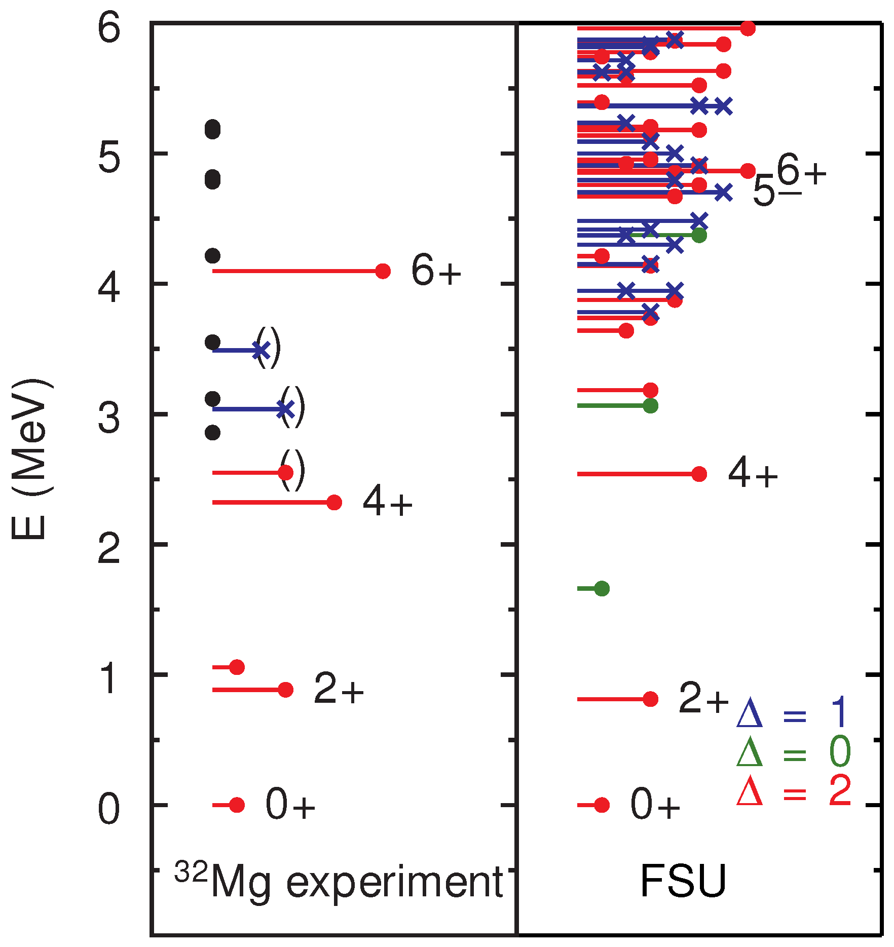
The (-shell) part of the FSU spectrum for Si (the green lines in Figure 5) has a simple interpretation. The ground state is dominated by the proton configuration. The 5.24 MeV 2 and the 6.47 MeV 3 states are dominated by the proton configuration. In the two-proton transfer experiment from S [63], a 2 state at 5.33 is observed that can be interpreted as two protons removed from to make . The 0+ state is predicted at 8.76 MeV. For the FSU Hamiltonian, all of these predictions are based on the USDB effective Hamiltonian [64]. The ESPE for the and proton states near Si are determined from the binding energies of Al, Si and P. Above 2.5 MeV the level density is dominated by the neutron and configurations. The states can be interpreted in terms of the low-lying 3/2 and 1/2 states of Si coupled to the low-lying 7/2 and 3/2 states of Si. The state with maximum spin-parity of 5 predicted at 5.12 MeV can be compared to the proposed experimental 5 state at 4.97 MeV [65]. The theoretical spectra from the mixed SDPF-U-Mix shown in [65] is similar to the FSU unmixed spectrum in Figure 5.
The FSU results for Mg are shown in Figure 6. Compared to Si, there is an inversion of the low-lying = 0 and = 2 configurations. For pure configurations, the reduced electric-quadrupole transition strength for 2 ( = 2) to 0 ( = 0) is zero. Experimentally, = 48 e fm compared to = 96(16) e fm; see Table 1 in [66]. An improved half-life for the 0 is important since it helps to determine the mixing.
One of the key experiments for Mg is the two-neutron transfer from Mg (t,p), where the first two 0 states were observed with approximately equal strength [67]. This observatiom has proven difficult to understand; see the references in [68]. Starting from a = 0 configuration for the Mg ground state, one can populate the = 0, 0 configuration in Mg by transfer and the = 2, 0 configuration by transfer. Macchiavelli et al. [68] analyzed the (t,p) cross sections by used centroid energies for the = 0,2,4 configurations of 1.4, 0.2 and 0.0 MeV, respectively, obtained with the SDPF-U-MIX Hamiltonian [60]. This three-level model could account for the experimental observation with a ground state that is 4% = 0, 46% = 2 and 40% = 4 together with a ground-state wavefunction for Mg that has 97% = 0 and 3% = 2. In this three-level model for Mg, the main part of the = 0 configuration is in the 0 state predicted to be near 2.2 MeV; see Table 1 in [68].
Two-proton knockout from Si provides more information. Starting with a pure = 0 configuration for the Si ground state, only = 0, 0 configurations in Mg can be made. In the two-proton knockout experiment of [69,70], strong 0 strength is observed in the sum of the first two 0 states; see Figure 9 in [70]. The strength to the 0 and 0 states cannot be separated due to the long lifetime of the 0 state. Significant strength to 0 states above 1.5 MeV was not observed, in contradiction to that predicted in the three-level model above [68] or the SDPF-M model. More needs to be done to understand the structure of Mg and how it connects to the experimental data discussed above.
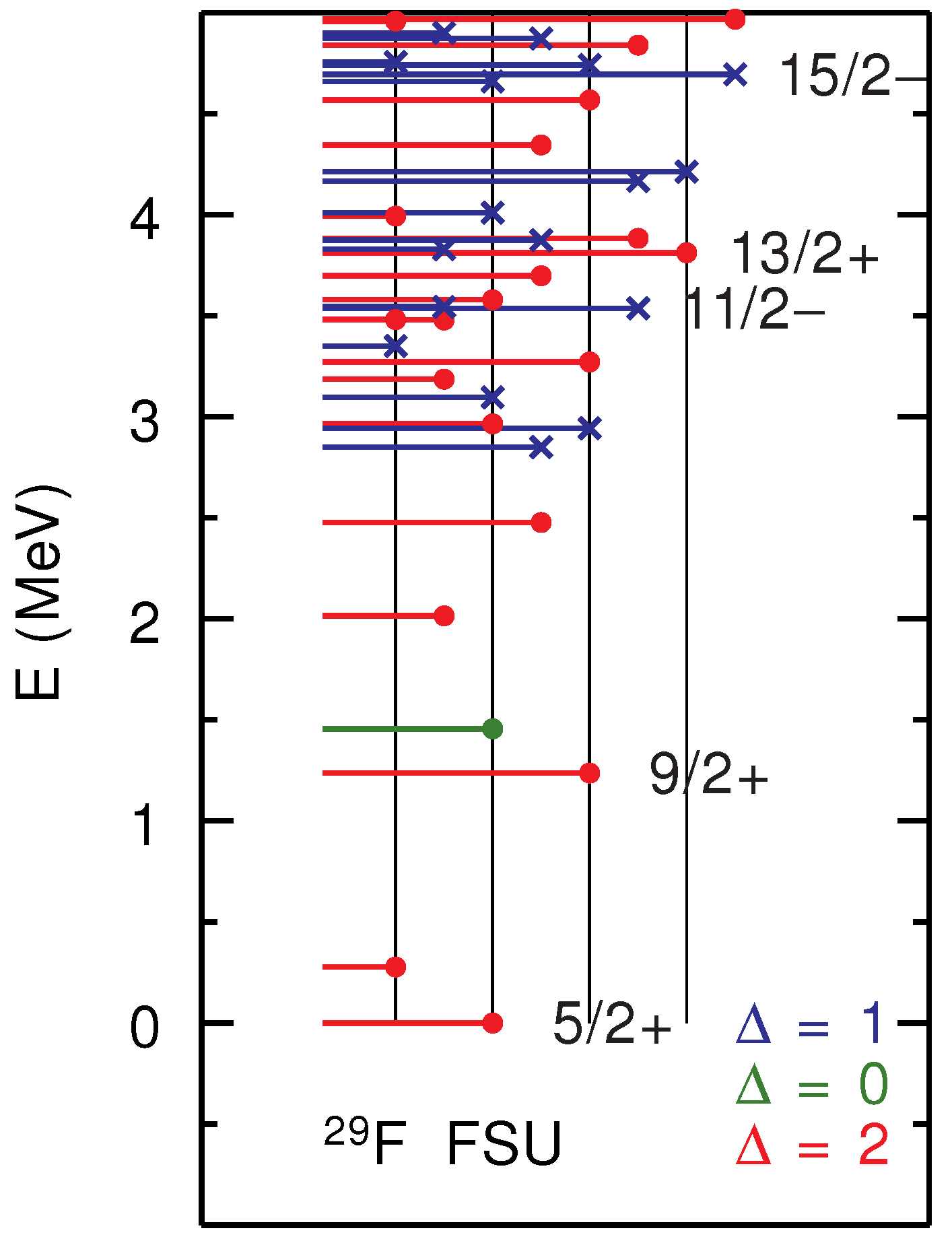
Results from the FSU Hamiltonian provide an extrapolation down to O. F has been called a “lighthouse on the island-of-inversion” [71]. The FSU results for F are shown in Figure 7. The lowest state is 5/2 with a configuration. The lowest 1/2, 3/2, 7/2 and 9/2 = 2 states are dominated by the configuration with coupled to the = 2, 2 state in O at 1.26 MeV. The coupled to 2, 5/2 configuration is spread over many higher 5/2 states in F. The states for F start at 3.9 MeV. An excited state in F at 1.080(18) MeV [72] made from proton knockout from Ne was suggested to be 1/2 on the basis comparisons to the SDPF-M calculations shown in [72].
With the FSU Hamiltonian, for F, the lowest = 0, 5/2 state is 1.9 MeV below the = 2, 5/2 state. The large FSU occupancy of 1.38 in F for the loosely bound orbital may explain the observed neutron halo [73]. In particular, the two-neutron transfer amplitudes TNA[(0p)]0.62 for the F, = 2, 5/2 ground state going to the F, = 0, 5/2 ground state. Improved mass mesurements are needed for the neutron-rich fluorine and neon isotopes.
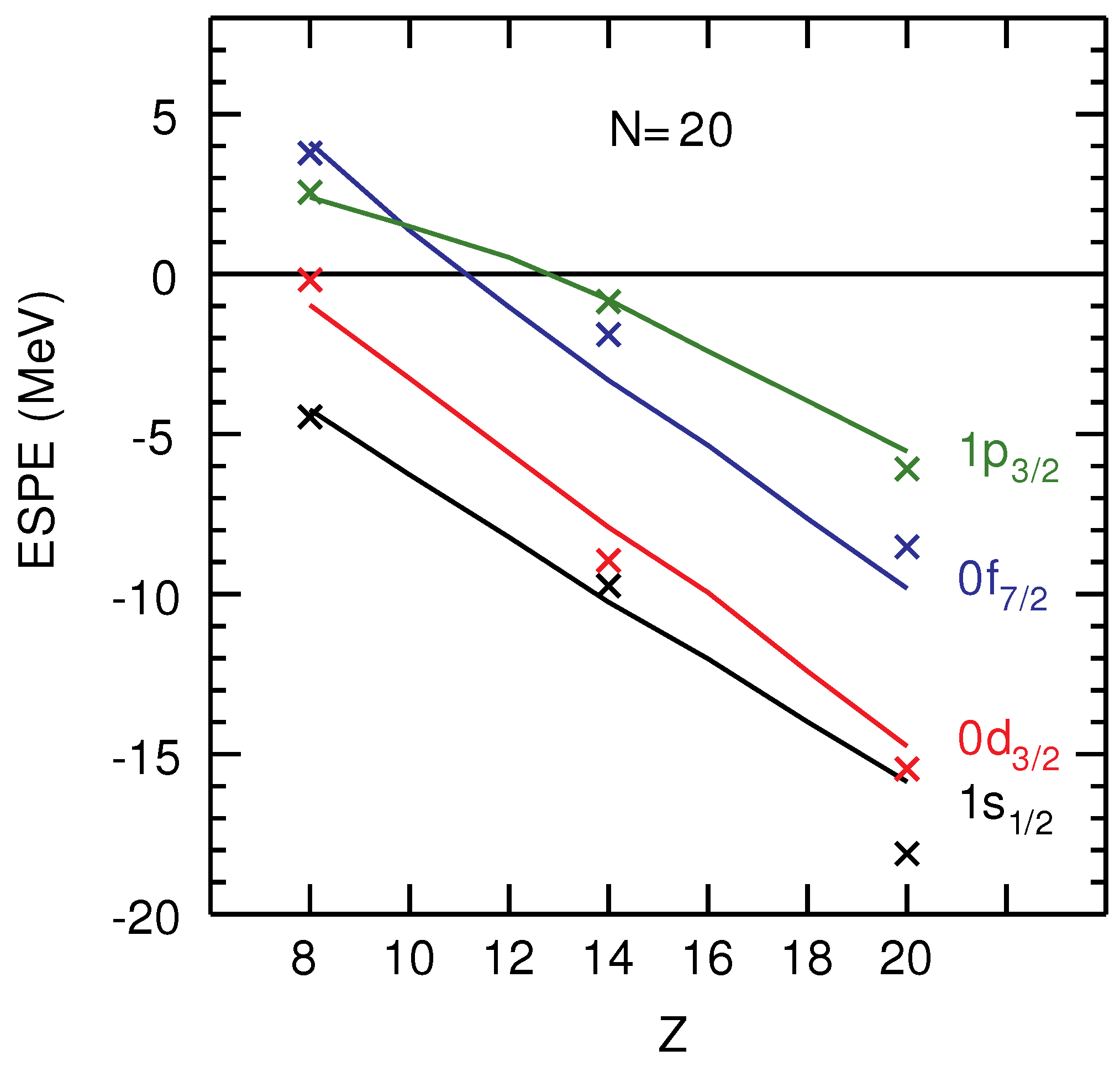
Results for these calculations depend on the ESPE extrapolation down to O contained in the FSU interaction. The ESPE for the neutron orbitals as a function of Z obtained with the FSU Hamiltonian with ( = 0) are shown in Figure 8 (for Si I assume a configuration for the protons). These are compared with the results from the Skyrme-x energy density functional (Skx EDF) calculations [74].
For unbound states, the energies can be approximated by first increasing the EDF central potential to obtain a wavefunction bound by, for example, 0.2 MeV, and then taking the expectation value of the wavefunction value with original EDF Hamiltonian. This method provides a practical approximation to the centroid energy. Results for the unbound resonances could be calculated more exactly from neutron scattering on the EDF potential.
The results in Figure 8 show that the shell gap decreases from approximately 7.0 MeV in Si to approximately 2.7 MeV in O. The major part of this decrease is due to the lowering energy for relative to as the states become more unbound. The energies for these two states cross at approximately . Recent experimental information on the ESPE near Mg and their interpretation similar to those of Figure 8 with a Woods–Saxon potential is given in [75]. For the FSU Hamiltonian, the loose binding effects are implicitly built into the monopole components of the TBME from the SVD fit to data on the BE and excitations energies.
There is also an increase in the gap in Si due to the proton-neutron tensor interaction contribution to the spin–orbit splitting [5] that is built into the FSU Hamiltonian. The spin–orbit tensor interacton is zero in the double- closed shell nuclei such as O and Ca. The tensor interaction is important for changing the effective single–particle energies as a function of proton and/or neutron number [5] or as a function of the state-dependent orbital occupancies [76].
The ESPE obtained from the Skx EDF [74] from Ne to Ni are shown in Figure 9. The energies of and systematically shift due to the finite-well potential.
For nuclei near the neutron drip line, there are few bound states that can be studied by their gamma decay. States above the neutron separation energy neutron decay. These neutron decays can be complex both experimentally and theoretically. The neutron decay spectrum depends upon how the unbound states are populated. They are often made by proton and neutron knockout reactions. For one- and two-nucleon knockout, one can calculate spectroscopic factors that can be combined with a reaction model to find which states are most strongly populated. A recent example of this type of calculation was for two-proton knockout from Mg going to Ne [77]. One neutron decay can often go to excited states in the daughter [77]. Additionally, multi-neutron decay can occur. It is important to measure the neutrons in coincidence with the final nucleus and its gamma decays. On the theoretical side, one must use the calculated wavefunctions to obtain neutron decay spectra.
An example of multi-neutron decay is in the one-proton knockout from F to make O [78,79]. The calculated one-proton knockout spectroscopic factors showed that knockout mainly leads to the ground state of O, and that knockout leads to many negative-parity states above the neutron separation energy of O. These excited states multi-neutron decay to O [78]. However, in the (p,2p) reaction [79], it was suggested from the momentum-distribution of O that a low-lying positive-parity excited state in O above the neutron separation energy was strongly populated by removal, in strong disagreement with the calculations of [78]. This experimental result should be confirmed.
The two-neutron decay of O has a remarkably small Q value of 0.018(5) MeV [50]. The theoretical Q value from USDC Hamiltonian [19] is 0.02(15) MeV. The decay width depends strongly on the ℓ for the two-nucleon decay amplitude. From Figure 2b of [80], pure two-nucleon decays widths with the experimental Q value are approximately 10, 10 and 10 MeV for ℓ = 0, 1 and 2, respectively. The calculated TNA in the model space with the USDC Hamiltonian are 0.99 for and 0.16 for . Thus, keV. The TNA will be on the order of TMBE , where is the energy difference between the the and states in O. With typical values of TMBE MeV and MeV [81] giving TNA = 0.5, the contribution to the two-neutron decay width will be small.
The nucleus O is unbound to four neutron decay. The theoretical understanding of this complex decay involves the four-body continuum [80]. These continuum calculations strongly depend upon the single-particle states involved; see Figure 2d in [80]. With the FSU Hamiltonian, the configuration for O lies 0.8 MeV below the (closed-shell) configuration due to the pairing correlations. The calculated four-neutron decay energy is 1.5 MeV. The energy should be lowered by an explicit treatment of the many-body continuum. Thus, the “island of inversion” may be a “peninsula of inversion” extending from Mg all the way to the neutron drip line; below, I discuss what may be the first true “island of inversion” between Ca and Ni. There are many paths for the four-neutron decay of O. For example, in the FSU model, it may proceed by a relatively fast decay to the O ground state followed by its decay to O.
3. The Region of Si
In this Section, results for two often used effective Hamiltonians for this model space, called SDPF-MU [82] and SDFP-U-SI [83], together with those based on the IMSRG method [20] are compared. The MU and U-SI Hamiltonians are “universal” in the sense that a single Hamiltonian with a smooth mass-dependence is applied to a wide mass region. MU is used for all nuclei in this model space, while U-SI was designed for (the SDPF-U version was designed for [83]).
The 2 energy in Si (0.74 MeV) is low compared to those in Si [14,20] (3.33 MeV) and Ca [20,28] (3.83 MeV). Si and Ca are doubly magic due to the magic number 20. Si [14,14] has a known intrinsic oblate deformation [84].
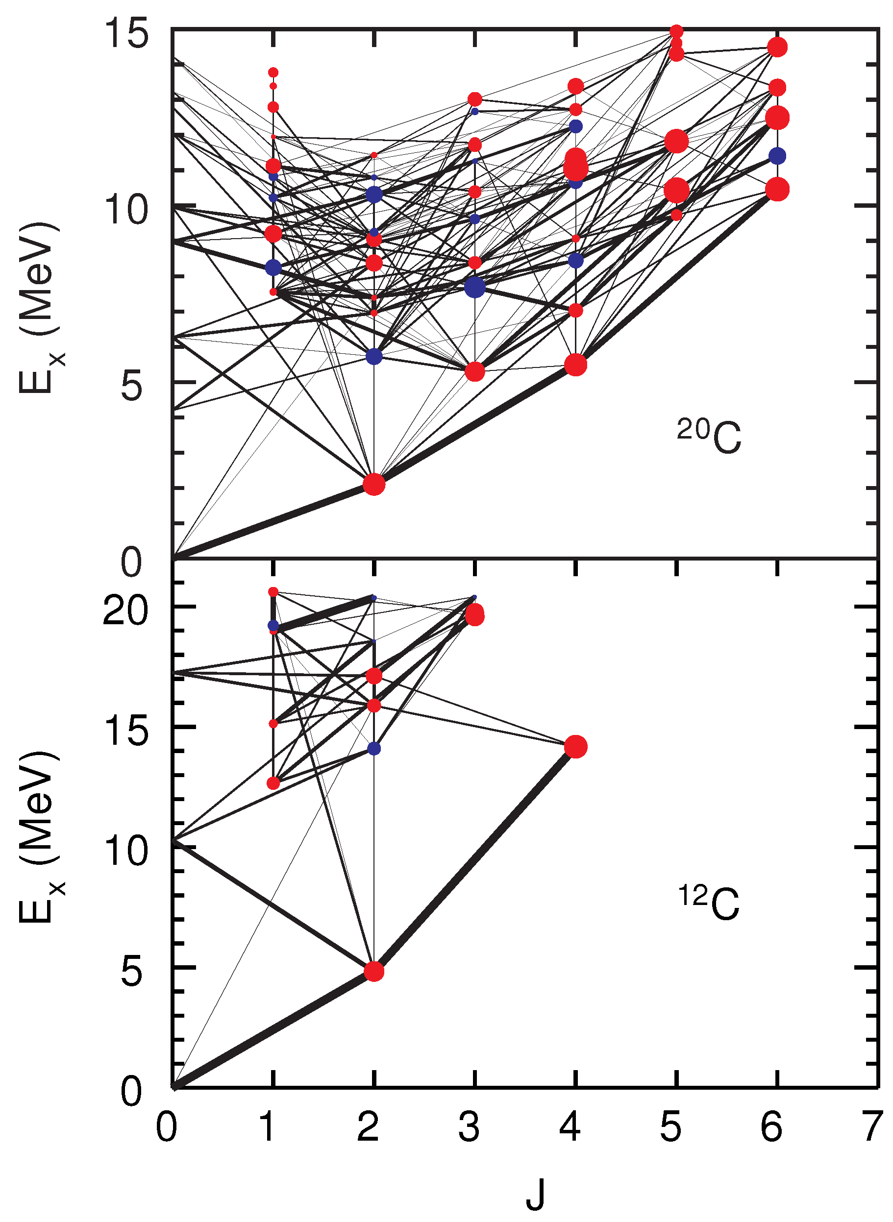
The 2 energy in C [6,14] (1.62 MeV) is low compared to those in C [6,8] (7.01 MeV) and O [8,14] (3.20 MeV). C and O are doubly magic due to the magic number 8. Hartree–Fock calculations [85] as well as CI calculations for the Q moment within the model space [86] show that C and C have intrinsic oblate shapes.
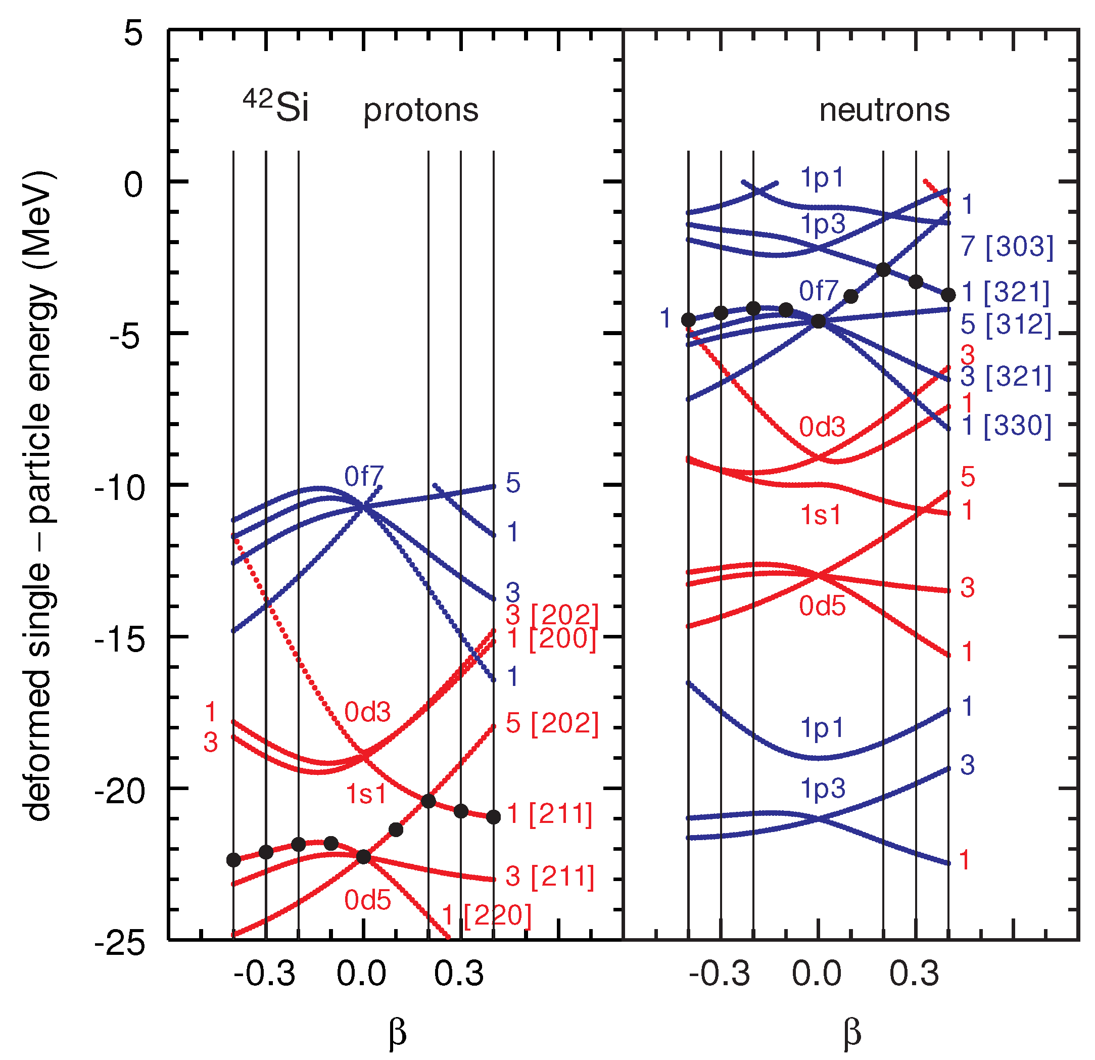
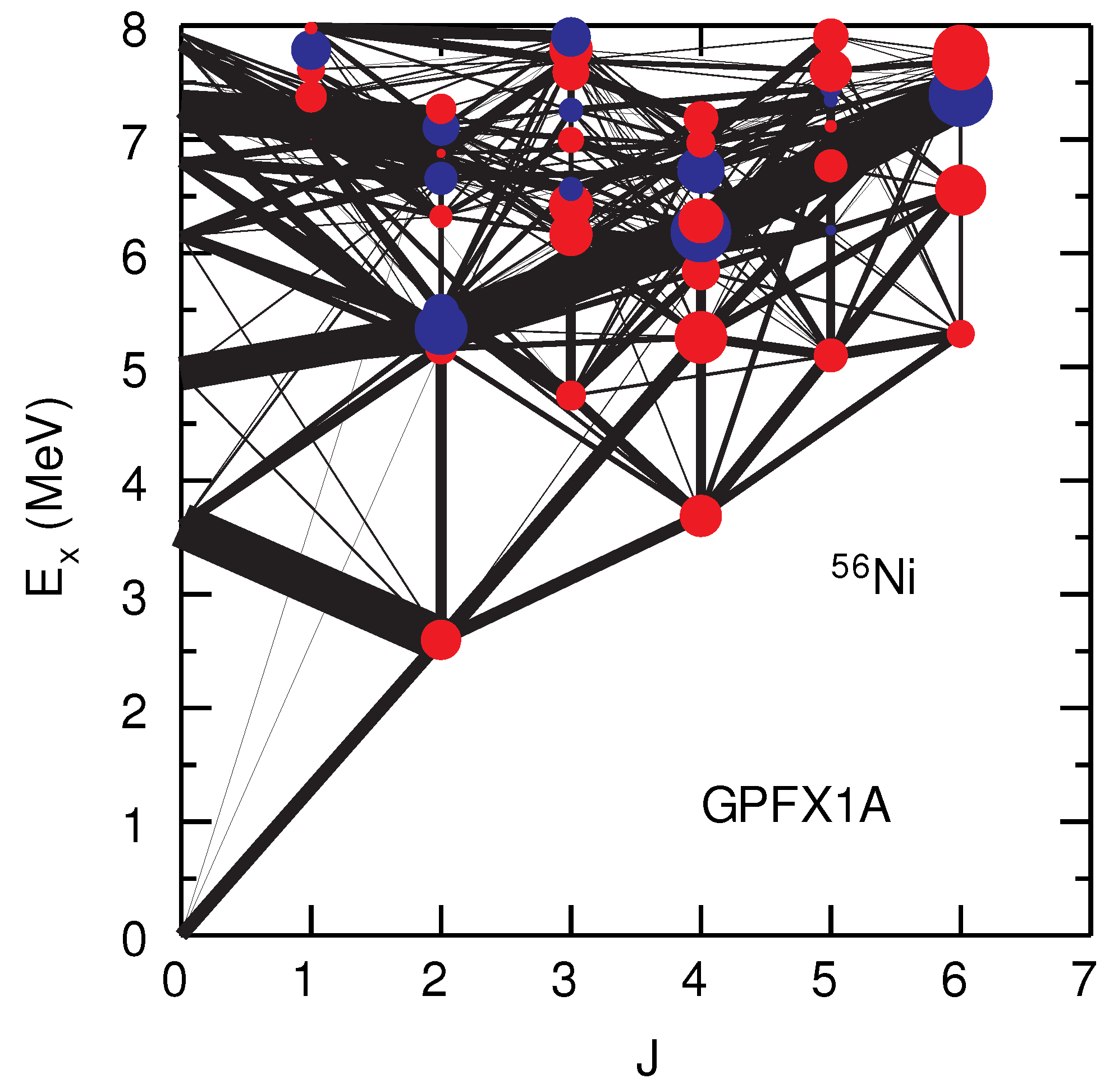
The oblate shapes for Si and Si are shown by their maps in Figure 10 and Figure 11. The transition from spherical to oblate shapes for the doubly-magic numbers can be qualitatively understood in the Nilsson diagram as shown, for example, for Si in Figure 12. The highest filled Nilsson orbitals have rather flat energies between = 0 and = −0.3. The important aspect is the concave bend of the 2 [N,n,] = 1 [2,2,0] proton and 1 [3,3,0] neutron Nilsson orbitals for oblate shapes. For the heavier doubly-magic nuclei, ℓ increases and the orbital decreases in energy, the bend will not be so large and the energy minima come closer to = 0. This is illustrated in Figure 10. In Figure 10a and Figure 10c, the spin–orbit gap is small enough to give an oblate rotational pattern. The oblate shape is manifest in the positive Q moments. In Figure 10a, the spin–orbit gap is increased by 1 MeV and the rotational energy pattern is broken. The pattern in Figure 10a is similar to that obtained for Ni in the model space as shown in Figure 13. An interesting feature for Ni is the relatively strong 0 to 2. I am not aware of a simple explanation for this.
The oblate bands in Si and Si are linked to the and orbitals. For completeness, the maps for C and C obtained with the WBP Hamiltonian [90] are shown in Figure 14. For these nuclei, the oblate ground-state bands are linked with the and orbitals.
For CI calculations, the values depend on the effective charge parameters and . In the harmonic-oscillator basis, the operator connects states within a major shell as well as those that change by two. The strength function contains low-lying strength as well “giant-quadrupole” strength near an energy of 2. The effective charges account for the renormalization of the proton and neutron components of the matrix elements within the CI basis of a major shell due to admixtures of the –, proton configurations. For the calculations, shown here, effective charges, which depend on the model space, are used. The effective charges are chosen to best reproduce observed values and quadrupole moments within that model space. These are the model space with and [91], the model space with [88] and the neutron-rich model space with [82]. Since low-lying excitations in nuclei are mostly isoscalar, only is well determined. It takes special situations such as a comparison of B(E2) in mirror nuclei [92] to obtain the isovector combination .
The isoscalar effective charge decreases for more neutron-rich nuclei (e.g., the drop from 0.5 in the model space to 0.35 in the model space). This can be understood by the macroscopic model of Mottelson [93], by the microscopic Hartree–Fock calculations of Sagawa et al. [85], and by the microscopic models, discussed in [94,95]. Microscopic models also give an orbital dependence to the effective charge. A recent example of this is for the relatively small B(E2) value for the the 1/2 to 5/2 transition in O [96]. This transition is dominated by the – matrix element, and the relatively small neutron effective charge is due to the node in the wavefunction.
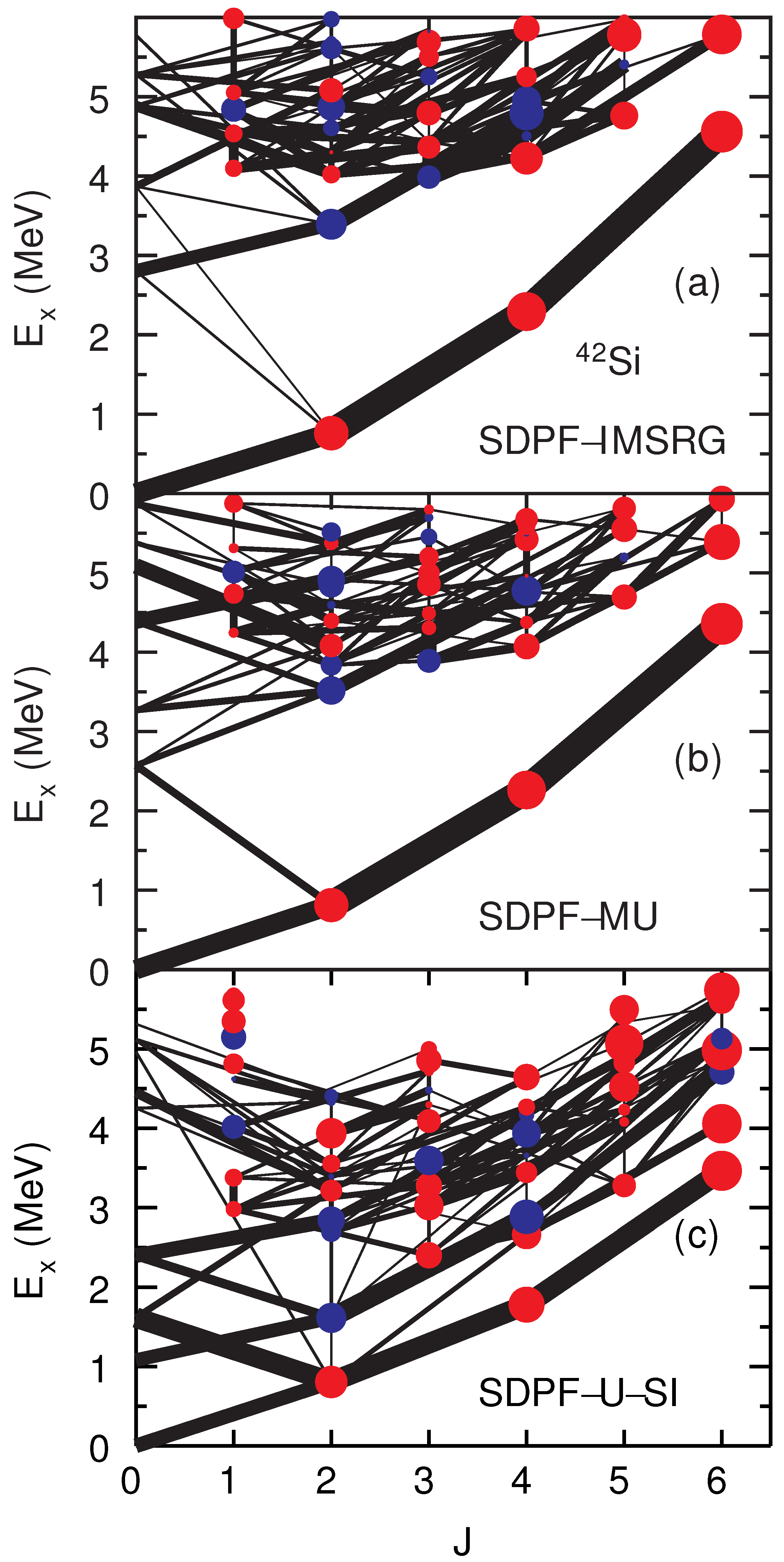
The results for CI calculations for Si are shown in Figure 11 for three Hamiltonians. The IMSRG Hamiltonian is based on a VS-IMSRG calculation [20] similar to that used in [12]. The interpretation of the spectroscopic quadrupole moments, , shown in Figure 11 in terms of an intrinsic shape, , is given by the rotational formula [97],
with the Nilsson quantum number for the ground-state bands in even–even nuclei. The MU [82] and IMSRG [20] calculations show an intrinsic oblate ground-state band, ( and ), followed by a large energy gap to other more complex states. The U-SI Hamiltonian [83] also gives an oblate ground-state band, but there is also an intrinsic prolate band at relatively low energy. The presence of this low-lying prolate band dramatically increases the level density below 4 MeV [98,99].
The Nilsson diagram in Figure 12 shows a higher-energy prolate minimum related to a crossing of the 1 [3,2,1] and 7 [3,0,3] Nilsson orbitals near = +0.3. At present, there is not enough experimental information to determine the energy of the prolate band in Si. The structure of Si is a touchstone for understanding all of the nuclei near the drip line in this mass region. More complete experimental results for the energy levels of Si are needed. The low-lying structure of Si depends on the details of the neutron ESPE that are affected by the continuum for the orbitals. The deformed neutron ESPE need to be established by one-neutron transfer reactions on Si.
Deformation for as a function of Z is determined by how the proton Nilsson orbitals are filled in Figure 12. When six protons are added to make Ca with , there is a sharp energy minimum for protons at = 0, and thus Ca is doubly magic. For S, the protons have a intrinsic prolate minimum near = +0.2 where the neutrons are near the crossing of the 2 = 1 and 7 orbitals [100]. In S, a K = 4 isomer at 2.27 MeV coming from the two quasi-particle state made from these two neutron orbitals was observed [101]. In S rotational bands associated with these, two states have been observed [102]. All of these features are reproduced by CI calculations based on the SDPF-MU [82] and SDPF-U [83] Hamiltonians. At higher excitation energy, the CI energy spectra are more complex than anything that could be easily understood by the collective model.
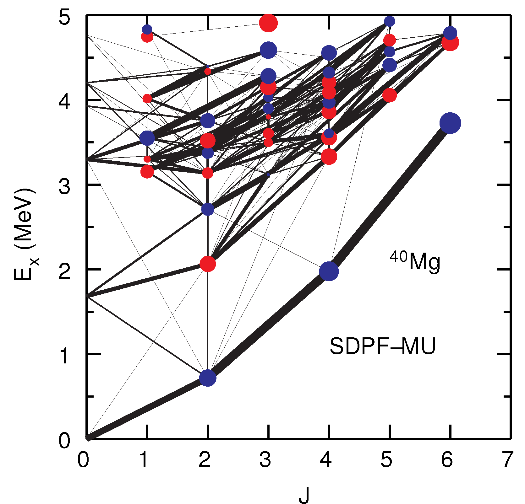
The map obtained with the SDPF-MU Hamiltonian for Mg is shown in Figure 15. In this case, the ground-state band has an intrinsic prolate shape. In the nuclear chart, prolate shapes are most common [103], in contrast to the oblate shapes obtained for magic numbers discussed above. The oblate shape for Mg can be understood in the Nilsson diagram of Figure 12. When two protons are removed, the energy minimum for protons shifts to positive in the 3 [2,1,1] orbital. The experimental energy of the first 2 is 500(14) keV [9] compared to the result of 718 keV obtained with the SDPF-MU Hamiltonian. Models that explicitly include the levels in the continuum are needed.
4. The Region of Ca
Many Hamiltonians have been developed for the calcium isotopes for the model space. Near Ca, it is known that – proton excitations are necessary for the low-lying intruder states and their mixing with the configurations which greatly increase the B(E2) values compared to those obtained in the model space [95]. In the doubly-magic nucleus Ca, the intruder states start with the 0 state at 4.28 MeV [104]. The Ca nuclei exhibit low-lying spectra which are dominated by configurations [12]. There are weak magic numbers at and 34 as shown in Figure 2. The reason for the low value of the pairing for the at was discussed in [104].
The KB3G [105] and GXPF1A [88,89] Hamiltonians have provided predictions for the spectra in this region which have been a source of comparison for many experiments over the last 20 years. Both of these are “universal” Hamiltonians for the model space. Recently, it has been shown that a data-driven Hamiltonian for the calcium isotopes improves the description of all of the known data [12]; this is called the UFP-CA (universal for calcium) Hamiltonian. All of the known energy data for can be described by an SVD-derived Hamiltonian that is close to the starting IMSRG Hamiltonian for Ca. UFP-CA is able to describe the energy data for with an rms error of 120 keV. In particular, the calculated values, shown by the red line in Figure 2, agree extremely well with the data (the black points).
The UFP-CA Hamiltonian does not explicitly involve the –– orbitals, but the influence of these orbitals are present in their contributions to the renormalization into the model space. This renormalization is contained microscopically in the IMSRG starting point, as well as empirically in the SVD fit.
The success of UFA-CA is similar to the success of the USD-type Hamiltonians in the model space for all nuclei except those in the island of inversion. If the UFP-CA predictions for Ca turn out to be in relatively good agreement with experiment, the implication is that Ca will be a doubly-magic nucleus similar to that of Ni [12]. If that is the case, Ca will be the last doubly-magic nucleus to be discovered. In [12], EDF models are used to estimate the shell gap at to be approximately 3.0 MeV. The implication of this for is shown by the red dashed line in Figure 2. The orbital will first appear as intruder states in the low-lying spectra of Ca. These nuclei can be reached by proton knockout on the scandium and titatium isotopes. The proton knockout will be dominated by removal to the low-lying neutron configurations. An example of this is the population of the ground state of Ca from Sc [106]. Protons will also be removed from the and orbitals to populate states at higher energy such as the negative parity state in Ca. These will mix with the –– configurations and neutron decay to the lighter calcium isotopes. For example, in Ca, a 9/2 () state just above the neutron separation energy value would neutron decay to the (0, 2, 4) multiplet predicted in Ca; see Figure 1 in [12]. Calculations that include proton excited from to and neutrons excited from to will be needed to understand the neutron dacays of these states.
The position of the orbital is crucial for the structure of nuclei around Ca [107]. Lenzi et al. [108] have extrapolated the neutron effective single-particle energies from down to based on their LNPS Hamiltonian. Their - ESPE gap for Ca is close to zero (see Figure 1 in [108]) and the structure of Ca is dominated by ( to ) configurations (see Table 1 in [108]). With LNPS, Ca is very different from Ni which is dominated by the closed -shell configuration ( = 0). Below Ni, the nuclei Fe, [11]Cr [11] and Ti [10], have deformed spectra coming from island of inversion for . Calculations with the LNPS Hamiltonian [108] show that these are all dominated by = 4. The island of inversion is the topic of another contribution to this series of papers [109].
The existence of Ca, confirmed only recently, agrees with UFP-CA as well as with most of the other predictions [36]. It will be exciting to have more complete experimental data for nuclei around Ca from FRIB and other radioactive-beam facilities.
5. The Region of Ni
Ni has recently been established as a double- magic nucleus from the relatively high energy of 2.6 MeV for the 2 state [35]. More detailed magic properties can be obtained from the and , derived from new experiments on the masses around Ni. The ESPE can be established from the masses together with the low-lying spectra of Ni, Ni, Co and Cu. A proton knockout experiment from Zn has recently been used to establish excitation energies of low-lying states in Cu [35] In particular, the ground state and two lowest-lying states are likely associated with the triplet of states shown in Figure 9. In comparison with the extrapolations of CI calculations, shown in [35], the order is likely to be , and . The single-particle nature of low-lying states around Ni will require one-nucleon transfer experiments.
The position of the proton orbital above Ni is important for Gamow–Teller strength in the electron-capture rates for core-collapse supernovae similations [110,111]. The filling of the orbital leads to Sn on the proton drip line. Sn has the largest calculated reduced Gamow-Teller transition probability, , value (see Table A1 in [112]) due to nearly filled orbital decaying into the nearly empty orbital. The understanding of Sn [113] and other nuclei near the proton drip line in this mass region will be improved by radioactive-beam experiments.
As shown in Figure 4b of [35], large-scale CI calculations predict a deformed band with at approximately 2.6 MeV. Ni is also spherical with a 2 state observed at 2.7 MeV. For Ni, the deformed band is predicted to start at 5.0 MeV as shown in Figure 13. The relatively low-lying deformed band in Ni is predicted to lead to a “5th island-of-inversion” in Fe and other nuclei with below [114].
6. Conclusions
I have discussed the new physics related to the properties of nuclei near the drip lines that will be studied by the next generation of rare-isotope beam experiments. In particular, I have focused on four “outposts” for the regions of O, Si, Ca and Ni, where new experiments will have the greatest impact on understanding the evolution of nuclear struture as one approaches the neutron drip line.
Funding
This research was funded by the National Science Foundation under Grant PHY-2110365.
Acknowledgments
I thank Ragnar Stroberg for providing the VS-IMSRG Hamiltonian for Si.
Conflicts of Interest
The author declares no conflict of interest.
References
- Brown, B.A.; Wildenthal, B.H. Status of the nuclear shell model. Ann. Rev. Nucl. Part. Sci. 1988, 38, 29–66. [Google Scholar] [CrossRef]
- Brown, B.A. The nuclear shell model towards the drip lines. Prog. Part. Nucl. Phys. 2001, 47, 517–599. [Google Scholar] [CrossRef]
- Caurier, E.; Martinez-Pinedo, G.; Nowacki, F.; Poves, A.; Zuker, A. The shell model as a unified view of nuclear structure. Rev. Mod. Phys. 2005, 77, 427–488. [Google Scholar] [CrossRef] [Green Version]
- Stroberg, S.R.; Hergert, H.; Bogner, S.K.; Holt, J.D. Nonempirical interactions for the nuclear shell model: An update. Ann. Rev. Nucl. Part. Sci. 2019, 69, 307–362. [Google Scholar] [CrossRef] [Green Version]
- Otsuka, T.; Gade, A.; Sorlin, O.; Suzuki, T.; Utsuno, Y. Evolution of shell structure in exotic nuclei. Rev. Mod. Phys. 2020, 92, 015002. [Google Scholar] [CrossRef] [Green Version]
- Brown, B.A. Nuclear pairing gap: How low can it go? Phys. Rev. Lett. 2013, 111, 162502. [Google Scholar] [CrossRef] [Green Version]
- Audi, G. The history of nuclidic masses and of their evaluation. Int. J. Mass Spec. 2006, 251, 85–94. [Google Scholar] [CrossRef] [Green Version]
- Pritychenko, B.; Birch, M.; Singh, B.; Horoi, M. Tables of E2 transition probabilities from the first 2+ states in even-even nuclei. Atom. Data Nucl. Data Tables 2016, 107, 1–139. [Google Scholar] [CrossRef] [Green Version]
- Crawford, H.L.; Fallon, P.; Macchiavelli, A.O.; Doornenbal, P.; Aoi, N.; Browne, F.; Campbell, C.M.; Chen, S.; Clark, R.M.; Cortes, M.L.; et al. First spectroscopy of the near drip-line nucleus 40Mg. Phys. Rev. Lett. 2019, 122, 052501. [Google Scholar] [CrossRef] [Green Version]
- Cortes, M.L.; Rodriguez, W.; Doornenbal, P.; Obertelli, A.; Holt, J.D.; Lenzi, S.M.; Menendez, J.; Nowacki, F.; Ogata, K.; Poves, A.; et al. Shell evolution of N = 40 isotones towards 60Ca: First spectroscopy of 62Ti. Phys. Lett. B 2020, 800, 135071. [Google Scholar] [CrossRef]
- Santamaria, C.; Louchart, C.; Obertelli, A.; Werner, V.; Doornenbal, P.; Nowacki, F.; Authelet, G.; Baba, H.; Calvet, D.; Chateau, F.; et al. Extension of the N = 40 island of inversion towards N = 50: Spectroscopy of 66Cr, 70Fe, 72Fe. Phys. Rev. Lett. 2015, 115, 192501. [Google Scholar] [CrossRef] [PubMed] [Green Version]
- Magilligan, A.; Brown, B.A.; Stroberg, S.R. Data-driven configuration-interaction Hamiltonian extrapolation to 60Ca. Phys. Rev. C 2021, 104, L051302. [Google Scholar] [CrossRef]
- Mass Explorer. Available online: http://massexplorer.frib.msu.edu/ (accessed on 10 April 2022).
- Morris, T.D.; Simonis, J.; Stroberg, S.R.; Stumpf, C.; Hagen, G.; Holt, J.D.; Jansen, G.R.; Papenbrock, T.; Roth, R.; Schwenk, A. Structure of the lightest tin isotopes. Phys. Rev. Lett. 2018, 120, 152503. [Google Scholar] [CrossRef] [PubMed] [Green Version]
- Warburton, E.K.; Becker, J.A.; Brown, B.A. Mass systematics for A = 29–44 nuclei: The deformed A∼32 region. Phys. Rev. C 1990, 41, 1147–1166. [Google Scholar] [CrossRef] [Green Version]
- Serduke, F.J.D.; Lawson, R.D.; Gloeckner, D.H. Shell-model study of N = 49 isotones. Nucl. Phys. A 1976, 256, 45–86. [Google Scholar] [CrossRef]
- Ji, X.D.; Wildenthal, B.H. Shell-model calculations for the energy-levels of the N = 50 isotones with A = 80–87. Phys. Rev. C 1989, 40, 389–398. [Google Scholar] [CrossRef]
- Lisetskiy, A.; Brown, B.; Horoi, M.; Grawe, H. New T = 1 effective interactions for the f5/2p3/2p1/2g9/2 model space: Implications for valence-mirror symmetry and seniority isomers. Phys. Rev. C 2004, 70, 044314. [Google Scholar] [CrossRef] [Green Version]
- Magilligan, A.; Brown, B.A. New isospin-breaking “USD” Hamiltonians for the sd shell. Phys. Rev. C 2020, 101, 064312. [Google Scholar] [CrossRef]
- Stroberg, S.R.; Holt, J.D.; Schwenk, A.; Simonis, J. Ab initio limits of atomic nuclei. Phys. Rev. Lett. 2021, 126, 022501. [Google Scholar] [CrossRef]
- Forssén, C.; Hagen, G.; Hjorth-Jensen, M.; Nazarewicz, W.; Rotureau, J. Living on the edge of stability, the limits of the nuclear landscape. Physica Scripta 2013, 2013, 014022. [Google Scholar] [CrossRef] [Green Version]
- Rotureau, J.; Michel, N.; Nazarewicz, W.; Płoszajczak, M.; Dukelsky, J. Density matrix renormalization group approach for many-body open quantum systems. Phys. Rev. Lett. 2006, 97, 110603. [Google Scholar] [CrossRef] [PubMed] [Green Version]
- Rotureau, J.; Michel, N.; Nazarewicz, W.; Płoszajczak, M.; Dukelsky, J. Density matrix renormalization group approach to two-fluid open many-fermion systems. Phys. Rev. C 2009, 79, 014304. [Google Scholar] [CrossRef] [Green Version]
- Bertulani, C.; Hammer, H.W.; Van Kolck, U. Effective field theory for halo nuclei: Shallow p-wave states. Nucl. Phys. A 2002, 712, 37–58. [Google Scholar] [CrossRef] [Green Version]
- Bedaque, P.; Hammer, H.W.; Van Kolck, U. Narrow resonances in effective field theory. Phys. Lett. B 2003, 569, 159–167. [Google Scholar] [CrossRef] [Green Version]
- Id Betan, R.; Liotta, R.J.; Sandulescu, N.; Vertse, T. Two-particle resonant states in a many-body mean field. Phys. Rev. Lett. 2002, 89, 042501. [Google Scholar] [CrossRef] [Green Version]
- Michel, N.; Nazarewicz, W.; Płoszajczak, M.; Bennaceur, K. Gamow shell model description of neutron-rich nuclei. Phys. Rev. Lett. 2002, 89, 042502. [Google Scholar] [CrossRef] [Green Version]
- Michel, N.; Nazarewicz, W.; Płoszajczak, M.; Vertse, T. Shell model in the complex energy plane. J. Phys. G: Nucl Part. Phys. 2009, 36, 013101. [Google Scholar] [CrossRef] [Green Version]
- Berggren, T.; Lind, P. Resonant state expansion of the resolvent. Phys. Rev. C 1993, 47, 768–778. [Google Scholar] [CrossRef]
- Lind, P. Completeness relations and resonant state expansions. Phys. Rev. C 1993, 47, 1903–1920. [Google Scholar] [CrossRef]
- Volya, A.; Zelevinsky, V. Discrete and continuum spectra in the unified shell model approach. Phys. Rev. Lett. 2005, 94, 052501. [Google Scholar] [CrossRef] [Green Version]
- Li, J.; Ma, Y.; Michel, N.; Hu, B.; Sun, Z.; Zuo, W.; Xu, F. Recent progress in Gamow shell model calculations of drip line nuclei. Physics 2021, 3, 977–997. [Google Scholar] [CrossRef]
- Tanihata, I.; Savajols, H.; Kanungo, R. Recent experimental progress in nuclear halo structure studies. Prog. Part. Nucl. Phys. 2013, 68, 215–313. [Google Scholar] [CrossRef]
- Tanihata, I.; Hamagaki, H.; Hashimoto, O.; Shida, Y.; Yoshikawa, N.; Sugimoto, K.; Yamakawa, O.; Kobayashi, T.; Takahashi, N. Measurements of interaction cross-sections and nuclear radii in the light p-shell region. Phys. Rev. Lett. 1985, 55, 2676–2679. [Google Scholar] [CrossRef] [PubMed] [Green Version]
- Olivier, L.; Franchoo, S.; Niikura, M.; Vajta, Z.; Sohler, D.; Doornenbal, P.; Obertelli, A.; Tsunoda, Y.; Otsuka, T.; Authelet, G.; et al. Persistence of the Z = 28 shell gap around 78Ni: First spectroscopy of 79Cu. Phys. Rev. Lett. 2017, 119, 192501. [Google Scholar] [CrossRef] [Green Version]
- Tarasov, O.B.; Ahn, D.S.; Bazin, D.; Fukuda, N.; Gade, A.; Hausmann, M.; Inabe, N.; Ishikawa, S.; Iwasa, N.; Kawata, K.; et al. Discovery of 60Ca and implications for the stability of 70Ca. Phys. Rev. Lett. 2018, 121, 022501. [Google Scholar] [CrossRef] [Green Version]
- Brown, B.A.; Blank, B.; Giovinazzo, J. Hybrid model for two-proton radioactivity. Phys. Rev. C 2019, 100, 054332. [Google Scholar] [CrossRef]
- Jin, Y.; Niu, C.Y.; Brown, K.W.; Li, Z.H.; Hua, H.; Anthony, A.K.; Barney, J.; Charity, R.J.; Crosby, J.; Dell’Aquila, D.; et al. First observation of the four-proton unbound nucleus 18Mg. Phys. Rev. Lett. 2021, 127, 262502. [Google Scholar] [CrossRef]
- Tostevin, J.A.; Gade, A. Updated systematics of intermediate-energy single-nucleon removal cross sections. Phys. Rev. C 2021, 103, 054610. [Google Scholar] [CrossRef]
- Paschalis, S.; Petri, M.; Macchiavelli, A.O.; Hen, O.; Piasetzky, E. Nucleon-nucleon correlations and the single-particle strength in atomic nuclei. Phys. Lett. B 2020, 800, 135110. [Google Scholar] [CrossRef]
- Hen, O.; Miller, G.A.; Piasetzky, E.; Weinstein, L.B. Nucleon-nucleon correlations, short-lived excitations, and the quarks within. Rev. Mod. Phys. 2017, 89, 045002. [Google Scholar] [CrossRef] [Green Version]
- Panin, V.; Taylor, J.T.; Paschalis, S.; Wamers, F.; Aksyutina, Y.; Alvarez-Pol, H.; Aumann, T.; Bertulani, C.A.; Boretzky, K.; Caesar, C.; et al. Exclusive measurements of quasi-free proton scattering reactions in inverse and complete kinematics. Phys. Lett. B 2016, 753, 204–210. [Google Scholar] [CrossRef]
- Jensen, O.; Hagen, G.; Hjorth-Jensen, M.; Brown, B.A.; Gade, A. Quenching of spectroscopic factors for proton removal in oxygen isotopes. Phys. Rev. Lett. 2011, 107, 032501. [Google Scholar] [CrossRef] [PubMed] [Green Version]
- Wylie, J.; Okołowicz, J.; Nazarewicz, W.; Płoszajczak, M.; Wang, S.M.; Mao, X.; Michel, N. Spectroscopic factors in dripline nuclei. Phys. Rev. C 2021, 104, L061301. [Google Scholar] [CrossRef]
- Brown, B.A. The oxygen isotopes. Int. J. Mod. Phys. E 2017, 26, 1740003. [Google Scholar] [CrossRef]
- Wildenthal, B.H. Empirical strengths of spin operators in nuclei. Prog. Part. Nucl. Phys. 1984, 11, 5–51. [Google Scholar] [CrossRef]
- Kanungo, R.; Nociforo, C.; Prochazka, A.; Aumann, T.; Boutin, D.; Cortina-Gil, D.; Davids, B.; Diakaki, M.; Farinon, F.; Geissel, H.; et al. One-neutron removal measurement reveals 24O as a new doubly magic nucleus. Phys. Rev. Lett. 2009, 102, 152501. [Google Scholar] [CrossRef] [PubMed]
- Hoffman, C.R.; Baumann, T.; Bazin, D.; Brown, J.; Christian, G.; Denby, D.H.; DeYoung, P.A.; Finck, J.E.; Frank, N.; Hinnefeld, J.; et al. Evidence for a doubly magic 24O. Phys. Lett. B 2009, 672, 17–21. [Google Scholar] [CrossRef] [Green Version]
- Janssens, R.V.F. Unexpected doubly magic nucleus. Nature 2009, 459, 1069–1070. [Google Scholar] [CrossRef]
- Kondo, Y.; Nakamura, T.; Tanaka, R.; Minakata, R.; Ogoshi, S.; Orr, N.A.; Achouri, N.L.; Aumann, T.; Baba, H.; Delaunay, F.; et al. Nucleus 26O: A barely unbound system beyond the drip line. Phys. Rev. Lett. 2016, 116, 102503. [Google Scholar] [CrossRef] [Green Version]
- Thibault, C.; Klapisch, R.; Rigaud, C.; Poskanzer, A.M.; Prieels, R.; Lessard, L.; Reisdorf, W. Direct measurement of the masses of 11Li and 26–32Na with an on-line mass spectrometer. Phys. Rev. C 1975, 12, 644–657. [Google Scholar] [CrossRef] [Green Version]
- Campi, X.; Flocard, H.; Kerman, A.K.; Koonin, S. Shape transition in the neutron rich sodium isotopes. Nucl. Phys. A 1975, 251, 193–205. [Google Scholar] [CrossRef]
- Wildenthal, B.H.; Chung, W. Collapse of the conventional shell-model ordering in the very-neutron-rich isotopes of Na and Mg. Phys. Rev. C 1980, 22, 2260–2262. [Google Scholar] [CrossRef]
- Wildenthal, B.H.; Curtin, M.S.; Brown, B.A. Predicted features of the decay-decay of neutron-rich sd-shell nuclei. Phys. Rev. C 1983, 28, 1343–1366. [Google Scholar] [CrossRef]
- Poves, A.; Retamosa, J. The onset of deformation at the N = 20 neutron shell closure far from stability. Phys. Lett. B 1987, 184, 311–315. [Google Scholar] [CrossRef]
- Lubna, R.S.; Kravvaris, K.; Tabor, S.L.; Tripathi, V.; Volya, A.; Rubino, E.; Allmond, J.M.; Abromeit, B.; Baby, L.T.; Hensley, T.C. Structure of 38Cl and the quest for a comprehensive shell model interaction. Phys. Rev. C 2019, 100, 034308. [Google Scholar] [CrossRef] [Green Version]
- Brown, B.A.; Rae, W.D.M. The Shell-model code NuShellX@MSU. Nucl. Data Sheets 2014, 120, 115–118. [Google Scholar] [CrossRef]
- Gloeckner, D.H.; Lawson, R.D. Spurious center-of-mass motion. Phys. Lett. B 1974, 53, 313–318. [Google Scholar] [CrossRef]
- Brown, B.A.; Etchegoyen, A.; Godwin, N.S.; Rae, W.D.M.; Richter, W.A.; Ormand, W.E.; Warburton, E.K.; Winfield, J.S.; Zhao, L.; Zimmerman, C.H. Oxbash for Windows PC; MSU-NSCL Report 1289; National Superconducting Cyclotron Laboratory MSU: East Lansing, MI, USA, 2004. [Google Scholar]
- Caurier, E.; Nowacki, F.; Poves, A. Merging of the islands of inversion at N = 20 and N = 28. Phys. Rev. C 2014, 90, 014302. [Google Scholar] [CrossRef] [Green Version]
- Utsuno, Y.; Otsuka, T.; Mizusaki, T.; Honma, M. Varying shell gap and deformation in N∼20 unstable nuclei studied by the Monte Carlo shell model. Phys. Rev. C 1999, 60, 054315. [Google Scholar] [CrossRef]
- Otsuka, T.; Honma, M.; Mizusaki, T.; Shimizu, N.; Utsuno, Y. Monte Carlo shell model for atomic nuclei. Prog. Part. Nucl. Phys. 2001, 47, 319–400. [Google Scholar] [CrossRef]
- Fifield, L.K.; Woods, C.L.; Bark, R.A.; Drumm, P.V.; Hotchkis, M.A.C. Masses and level schemes of 33Si and 34Si. Nucl. Phys. A 1985, 440, 531–542. [Google Scholar] [CrossRef]
- Brown, B.A.; Richter, W.A. New “USD” Hamiltonians for the sd shell. Phys. Rev. C 2006, 74, 034315. [Google Scholar] [CrossRef] [Green Version]
- Lica, R.; Rotaru, F.; Borge, M.J.G.; Grevy, S.; Negoita, F.; Poves, A.; Sorlin, O.; Andreyev, A.N.; Borcea, R.; Costache, C.; et al. Normal and intruder configurations in 34Si populated in the β− decay of 34Mg and 34Al. Phys. Rev. C 2019, 100, 034306. [Google Scholar] [CrossRef] [Green Version]
- Elder, R.; Iwasaki, H.; Ash, J.; Bazin, D.; Bender, P.C.; Braunroth, T.; Brown, B.A.; Campbell, C.M.; Crawford, H.L.; Elman, B.; et al. Intruder dominance in the 02+ state of 32Mg studied with a novel technique for in-flight decays. Phys. Rev. C 2019, 100, 041301. [Google Scholar] [CrossRef]
- Wimmer, K.; Kroell, T.; Kruecken, R.; Bildstein, V.; Gernhaeuser, R.; Bastin, B.; Bree, N.; Diriken, J.; Van Duppen, P.; Huyse, M.; et al. Discovery of the shape coexisting 0+ state in 34Mg by a two neutron transfer reaction. Phys. Rev. Lett. 2010, 105, 252501. [Google Scholar] [CrossRef] [Green Version]
- Macchiavelli, A.O.; Crawford, H.L.; Campbell, C.M.; Clark, R.M.; Cromaz, M.; Fallon, P.; Jones, M.D.; Lee, I.Y.; Salathe, M.; Brown, B.A.; et al. The 30Mg(t, p)32Mg “puzzle” reexamined. Phys. Rev. C 2016, 94, 051303. [Google Scholar] [CrossRef] [Green Version]
- Kitamura, N.; Wimmer, K.; Poves, A.; Shimizu, N.; Tostevin, J.A.; Bader, V.M.; Bancroft, C.; Barofsky, D.; Baugher, T.; Bazin, D.; et al. Coexisting normal and intruder configurations in 32Mg. Phys. Lett. B 2021, 822, 136682. [Google Scholar] [CrossRef]
- Kitamura, N.; Wimmer, K.; Miyagi, T.; Poves, A.; Shimizu, N.; Tostevin, J.A.; Bader, V.M.; Bancroft, C.; Barofsky, D.; Baugher, T.; et al. In-beam gamma-ray spectroscopy of 32Mg via direct reactions. Phys. Rev. C 2022, 105, 034318. [Google Scholar] [CrossRef]
- Fortunato, L.; Casal, J.; Horiuchi, W.; Singh, J.; Vitturi, A. The 29F nucleus as a lighthouse on the coast of the island of inversion. Nat. Comm. Phys. 2020, 3, 132. [Google Scholar] [CrossRef]
- Doornenbal, P.; Scheit, H.; Takeuchi, S.; Utsuno, Y.; Aoi, N.; Li, K.; Matsushita, M.; Steppenbeck, D.; Wang, H.; Baba, H.; et al. Low-Z shore of the “island of inversion” and the reduced neutron magicity toward 28O. Phys. Rev. C 2017, 95, 041301. [Google Scholar] [CrossRef] [Green Version]
- Bagchi, S.; Kanungo, R.; Tanaka, Y.K.; Geissel, H.; Doornenbal, P.; Horiuchi, W.; Hagen, G.; Suzuki, T.; Tsunoda, N.; Ahn, D.S.; et al. Two-neutron halo is unveiled in 29F. Phys. Rev. Lett. 2020, 124, 222504. [Google Scholar] [CrossRef] [PubMed]
- Brown, B. New Skyrme interaction for normal and exotic nuclei. Phys. Rev. C 1998, 58, 220–231. [Google Scholar] [CrossRef]
- MacGregor, P.T.; Sharp, D.K.; Freeman, S.J.; Hoffman, C.R.; Kay, B.P.; Tang, T.L.; Gaffney, L.P.; Baader, E.F.; Borge, M.J.G.; Butler, P.A.; et al. Evolution of single-particle structure near the N = 20 island of inversion. Phys. Rev. C 2021, 104, L051301. [Google Scholar] [CrossRef]
- Otsuka, T.; Tsunoda, Y. The role of shell evolution in shape coexistence. J. Phys. G: Nucl Part. Phys. 2016, 43, 024009. [Google Scholar] [CrossRef]
- Chrisman, D.; Kuchera, A.N.; Baumann, T.; Blake, A.; Brown, B.A.; Brown, J.; Cochran, C.; DeYoung, P.A.; Finck, J.E.; Frank, N.; et al. Neutron-unbound states in 31Ne. Phys. Rev. C 2021, 104, 034313. [Google Scholar] [CrossRef]
- Thoennessen, M.; Baumann, T.; Brown, B.A.; Enders, J.; Frank, N.; Hansen, R.G.; Heckman, P.; Luther, B.A.; Seitz, J.; Stolz, A.; et al. Single proton knock-out reactions from 24F, 25F, 26F. Phys. Rev. C 2003, 68, 044318. [Google Scholar] [CrossRef] [Green Version]
- Tang, T.L.; Uesaka, T.; Kawase, S.; Beaumel, D.; Dozono, M.; Fujii, T.; Fukuda, N.; Fukunaga, T.; Galindo-Uribarri, A.; Hwang, S.H.; et al. How different is the core of 25F from 24Og.s. ? Phys. Rev. Lett. 2020, 124, 212502. [Google Scholar] [CrossRef]
- Grigorenko, L.V.; Mukha, I.G.; Scheidenberger, C.; Zhukov, M.V. Two-neutron radioactivity and four-nucleon emission from exotic nuclei. Phys. Rev. C 2011, 84, 021303. [Google Scholar] [CrossRef] [Green Version]
- Lepailleur, A.; Wimmer, K.; Mutschler, A.; Sorlin, O.; Thomas, J.C.; Bader, V.; Bancroft, C.; Barofsky, D.; Bastin, B.; Baugher, T.; et al. Spectroscopy of 28Na: Shell evolution toward the drip line. Phys. Rev. C 2015, 92, 054309. [Google Scholar] [CrossRef] [Green Version]
- Utsuno, Y.; Otsuka, T.; Brown, B.A.; Honma, M.; Mizusaki, T.; Shimizu, N. Shape transitions in exotic Si and S isotopes and tensor-force-driven Jahn-Teller effect. Phys. Rev. C 2012, 86, 051301. [Google Scholar] [CrossRef] [Green Version]
- Nowacki, F.; Poves, A. New effective interaction for 0ℏω shell-model calculations in the sd–pf valence space. Phys. Rev. C 2009, 79, 014310. [Google Scholar] [CrossRef] [Green Version]
- Morris, L.; Jenkins, D.G.; Harakeh, M.N.; Isaak, J.; Kobayashi, N.; Tamii, A.; Adachi, S.; Adsley, P.; Aoi, N.; Bracco, A.; et al. Search for in-band transitions in the candidate superdeformed band in 28Si. Phys. Rev. C 2021, 104, 054323. [Google Scholar] [CrossRef]
- Sagawa, H.; Zhou, X.; Zhang, X.Z. Deformations and electromagnetic moments in carbon and neon isotopes. Phys. Rev. C 2004, 70, 054316. [Google Scholar] [CrossRef]
- Petri, M.; Fallon, P.; Macchiavelli, A.O.; Paschalis, S.; Starosta, K.; Baugher, T.; Bazin, D.; Cartegni, L.; Clark, R.M.; Crawford, H.L.; et al. Lifetime measurement of the 21+ state in 20C. Phys. Rev. Lett. 2011, 107, 102501. [Google Scholar] [CrossRef] [Green Version]
- Cwiok, S.; Dudek, J.; Nazarewicz, W.; Skalski, J.; Werner, T. Single-particle energies, wave-functions, quadrupole-moments and g-factors in an axially deformed Woods-Saxson potential with applications to the 2-center-type nuclear problems. Comp. Phys. Comm. 1987, 46, 379–399. [Google Scholar] [CrossRef]
- Honma, M.; Otsuka, T.; Brown, B.; Mizusaki, T. New effective interaction for pf-shell nuclei and its implications for the stability of the N = Z = 28 closed core. Phys. Rev. C 2004, 69, 034335. [Google Scholar] [CrossRef] [Green Version]
- Honma, M.; Otsuka, T.; Brown, B.; Mizusaki, T. Shell-model description of neutron-rich pf-shell nuclei with a new effective interaction GXPF1. Eur. Phys. J. A 2005, 25, 499–502. [Google Scholar] [CrossRef]
- Warburton, E.; Brown, B. Effective interactions for the 0p1s0d nuclear shell-model space. Phys. Rev. C 1992, 46, 923–944. [Google Scholar] [CrossRef]
- Richter, W.A.; Mkhize, S.; Brown, B.A. sd-shell observables for the USDA and USDB Hamiltonians. Phys. Rev. C 2008, 78, 064302. [Google Scholar] [CrossRef] [Green Version]
- du Rietz, R.; Ekman, J.; Rudolph, D.; Fahlander, C.; Dewald, A.; Moller, O.; Saha, B.; Axiotis, M.; Bentley, M.; Chandler, C.; et al. Effective charges in the fp shell. Phys. Rev. Lett. 2004, 93, 222501. [Google Scholar] [CrossRef] [Green Version]
- Bohr, A.; Mottelson, B.R. Nuclear Structure; W. A. Benjamin, Inc.: New York, NY, USA, 1975; Volume 2. [Google Scholar]
- Brown, B.A.; Arima, A.; McGrory, J.B. E2 core-polarization charge for nuclei near 16O and 40Ca. Nucl. Phys. A 1977, 277, 77–108. [Google Scholar] [CrossRef]
- Longfellow, B.; Weisshaar, D.; Gade, A.; Brown, B.A.; Bazin, D.; Brown, K.W.; Elman, B.; Pereira, J.; Rhodes, D.; Spieker, M. Quadrupole collectivity in the neutron-rich sulfur isotopes 38S, 40S, 42S, 44S. Phys. Rev. C 2021, 103, 054309. [Google Scholar] [CrossRef]
- Heil, S.; Petri, M.; Vobig, K.; Bazin, D.; Belarge, J.; Bender, P.; Brown, B.A.; Elder, R.; Elman, B.; Gade, A.; et al. Electromagnetic properties of 21O for benchmarking nuclear Hamiltonians. Phys. Lett. B 2020, 809, 135678. [Google Scholar] [CrossRef]
- Lobner, K.; Vetter, M.; Honig, V. Nuclear intrinsic quadrupole moments and deformation paramters. Atom. Data Nucl. Data Tables 1970, 7, 495–520. [Google Scholar] [CrossRef]
- Tostevin, J.A.; Brown, B.A.; Simpson, E.C. Two-proton removal from 44S and the structure of 42Si. Phys. Rev. C 2013, 87, 027601. [Google Scholar] [CrossRef] [Green Version]
- Gade, A.; Brown, B.A.; Tostevin, J.A.; Bazin, D.; Bender, P.C.; Campbell, C.M.; Crawford, H.L.; Elman, B.; Kemper, K.W.; Longfellow, B.; et al. Is the structure of 42Si understood? Phys. Rev. Lett. 2019, 122, 222501. [Google Scholar] [CrossRef] [Green Version]
- Utsuno, Y.; Shimizu, N.; Otsuka, T.; Yoshida, T.; Tsunoda, Y. Nature of Isomerism in Exotic Sulfur Isotopes. Phys. Rev. Lett. 2015, 114. [Google Scholar] [CrossRef] [Green Version]
- Santiago-Gonzalez, D.; Wiedenhoever, I.; Abramkina, V.; Avila, M.L.; Baugher, T.; Bazin, D.; Brown, B.A.; Cottle, P.D.; Gade, A.; Glasmacher, T.; et al. Triple configuration coexistence in 44S. Phys. Rev. C 2011, 83, 061305. [Google Scholar] [CrossRef] [Green Version]
- Longfellow, B.; Weisshaar, D.; Gade, A.; Brown, B.A.; Bazin, D.; Brown, K.W.; Elman, B.; Pereira, J.; Rhodes, D.; Spieker, M. Shape changes in the N = 28 island of inversion: Collective structures built on configuration-coexistingsStates in 43S. Phys. Rev. Lett. 2020, 125, 232501. [Google Scholar] [CrossRef]
- Sharon, Y.Y.; Benczer-Koller, N.; Kumbartzki, G.J.; Zamick, L.; Casten, R.F. Systematics of the ratio of electric quadrupole moments Q(21+) to the square root of the reduced transition probabilities B(E2;01+→21+) in even-even nuclei. Nucl. Phys. A 2018, 980, 131–142. [Google Scholar] [CrossRef]
- Brown, B.; Richter, W. Shell-model plus Hartree-Fock calculations for the neutron-rich Ca isotopes. Phys. Rev. C 1998, 58, 2099–2107. [Google Scholar] [CrossRef] [Green Version]
- Poves, A.; Sanchez-Solano, J.; Caurier, E.; Nowacki, F. Shell model study of the isobaric chains A = 50, A = 51 and A = 52. Nucl. Phys. A 2001, 694, 157–198. [Google Scholar] [CrossRef] [Green Version]
- Browne, F.; Chen, S.; Doornenbal, P.; Obertelli, A.; Ogata, K.; Utsuno, Y.; Yoshida, K.; Achouri, N.L.; Baba, H.; Calvet, D.; et al. Pairing forces govern population of doubly magic 54Ca from direct reactions. Phys. Rev. Lett. 2021, 126, 252501. [Google Scholar] [CrossRef] [PubMed]
- Bhoy, B.; Srivastava, P.C.; Kaneko, K. Shell model results for 47–58Ca isotopes in the fp, fpg9/2 and fpg9/2d5/2 model spaces. J. Phys. G: Nucl. Part. Phys. 2020, 47, 065105. [Google Scholar] [CrossRef] [Green Version]
- Lenzi, S.M.; Nowacki, F.; Poves, A.; Sieja, K. Island of inversion around Cr-64. Phys. Rev. C 2010, 82, 054301. [Google Scholar] [CrossRef]
- Gade, A. Reaching into the N = 40 Island of inversion with nucleon removal reactions. Physics 2021, 3, 1226–1236. [Google Scholar] [CrossRef]
- Zamora, J.C.; Zegers, R.G.T.; Austin, S.M.; Bazin, D.; Brown, B.A.; Bender, P.C.; Crawford, H.L.; Engel, J.; Falduto, A.; Gade, A.; et al. Experimental constraint on stellar electron-capture rates from the 88Sr(t,3He+γ)88Rb reaction at 115 MeV/u. Phys. Rev. C 2019, 100, 032801. [Google Scholar] [CrossRef] [Green Version]
- Titus, E.R.; Ney, E.M.; Zegers, R.G.T.; Bazin, D.; Belarge, J.; Bender, P.C.; Brown, B.A.; Campbell, C.M.; Elman, B.; Engel, J.; et al. Constraints for stellar electron-capture rates on 86Kr via the 86Kr(t,3He+γ)86Br reaction and the implications for core-collapse supernovae. Phys. Rev. C 2019, 100, 045805. [Google Scholar] [CrossRef] [Green Version]
- Stroberg, S.R. Beta decay in medium-mass nuclei with the in-medium similarity renormalization group. Particles 2021, 4, 521–535. [Google Scholar] [CrossRef]
- Lubos, D.; Park, J.; Faestermann, T.; Gernhaeuser, R.; Kruecken, R.; Lewitowicz, M.; Nishimura, S.; Sakurai, H.; Ahn, D.S.; Baba, H.; et al. Improved value for the Gamow-Teller strength of the 100Sn beta decay. Phys. Rev. Lett. 2019, 122, 222502. [Google Scholar] [CrossRef]
- Nowacki, F.; Poves, A.; Caurier, E.; Bounthong, B. Shape coexistence in 78Ni as the portal to the fifth island of inversion. Phys. Rev. Lett. 2016, 117, 272501. [Google Scholar] [CrossRef] [PubMed] [Green Version]
Figure 1.
Lower mass region of the nuclear chart. The colors indicate the energy of the first 2 state. In addition to the data from [8], recent data for Mn [9], Ti [10], Cr [11] and Fe [11] are added. The filled black circles show the doubly-magic nuclei associated with the most robust pairs of magic numbers 8, 20, 28 and 50. The small open circles show the doubly-magic nuclei associated with less robust magic numbers 6, 14, 16, 32, 34, and 40. The large open circles indicate the nuclei near the neutron drip lines that are the focus of this paper. The triangles are those nuclei observed to decay by two protons in the ground state. The cross indicates no magic number for protons or neutrons, and the question mark indicates that the doubly-magic status is not known.

Figure 2.
as given by Equation (1). The black dots with error bars are the experimental data. The blue crosses are the excitation energies of the 2 states. The orbitals that are being filled are shown. The red line is the results from the universal calcium (UFP-CA) Hamiltonian [12]. The dashed line is the extrapolation based on the universal nuclear energy density functional (version zero) (UNEDF0) binding energies. for Ca [13].

Figure 3.
The nuclear chart showing the magic numbers (see text for definition). The black lines show where the two-proton (upper) and two-neutron (lower) separation energies obtained with the universal nuclear energy density functional (version one) (UNEDF1) [13] cross 1 MeV. The filled red circles show the locations of double- magic nuclei established from experiment. The open red circle for Sn indicates a probably double- magic nucleus that has not been confirmed by experiment. The blue circles in the bottom left-hand side are nuclei in the double- magic number sequence that are oblate deformed.

Figure 4.
Lower mass region of the nuclear chart showing the magic numbers, 2, 8, 20 and 40 (see text for definitioon). The black lines show where the two-proton (upper) and two-neutron (lower) separation energies obtained with the UNEDF1 [13] functional cross 1 MeV. The filled red circles show the double- magic nuclei He, O and Ca. The open red circle for Ca indicates a possible doubly-magic nucleus that has not been confirmed by experiment. The green circles are doubly-magic nuclei associated with the j-orbital fillings. The blue lines indicate isotopes or isotones where the magic number is observed to be broken.

Figure 5.
Spectrum of Si obtained with the Florida State University (FSU) Hamiltonian [56] compared to experiment. The length of the horizontal lines are proportional to the the angular momentum, J. The experimental parity is indicated by blue for negative parity and red for positive parity. Experimental spin-parity, , values that are tentative are shown by “()”, and those with multiple of no assignments are shown by the black points. The calculated results are obtained with the FSU Hamiltonian with pure configurations. The parities are positive for (green) and (red) and negative for (blue).

Figure 6.
Spectrum of Mg obtained with the FSU Hamiltonian [56]. The results are obtained with pure configurations. The spins are proportional to the length of the horizontal lines. The parities are positive for (green) and (red) and negative for (blue).
Figure 6.
Spectrum of Mg obtained with the FSU Hamiltonian [56]. The results are obtained with pure configurations. The spins are proportional to the length of the horizontal lines. The parities are positive for (green) and (red) and negative for (blue).

Figure 7.
Spectrum of F obtained with the FSU Hamiltonian [56]. The results are obtained with pure configurations. The spins are proportional to the length of the horizontal lines. The parities are positive for (green) and (red) and negative for (blue).
Figure 7.
Spectrum of F obtained with the FSU Hamiltonian [56]. The results are obtained with pure configurations. The spins are proportional to the length of the horizontal lines. The parities are positive for (green) and (red) and negative for (blue).

Figure 8.
Effective single-particle energies (ESPE) for neutron orbitals as a function of proton number. The lines are from the Skyrme-x energy-density functional (Skx EDF) [74] calculations. The crosses are from the FSU [56] Hamiltonian calculations.

Figure 9.
ESPE for the proton (p) and neutron (n) orbitals obtained from the Skx EDF interaction [74] for a range of nuclei.
Figure 9.
ESPE for the proton (p) and neutron (n) orbitals obtained from the Skx EDF interaction [74] for a range of nuclei.

Figure 10.
Electric quadrupole () maps for Si. The results shown are based on the universal -shell version-B (USDB) Hamiltonian with (a) the spin–orbit energy gap increased by 1 MeV, (b) in the model space, and (c) with the spin–orbit energy gap decreased by 1 MeV. For each J value, ten states were calculated. The widths of the lines are proportional to the reduced electric quadrupole transition strength, . Lines for less than 5% of the largest value are not shown. The radius of the circles are proportional to spectroscopic quadrupole moment, (2). To set the scale, for panel (b) the 2 to 0 = 82 e fm and (2) = +19 e fm are used.

Figure 11.
maps for Si obtained with the SDPF-IMSRG [20] (a), SDPF-MU [82] (b), and SDPF-U-SI [83] (c) Hamiltonians. See Figure 10 and text for details.

Figure 12.
Nilsson diagram for Si. At the deformation parameter = 0, the orbitals are labeled by (see text for definitions), and, at larger deformation, the orbitals are labeled by the Nilsson quantum numbers 2 [N,n,]. The negative and positive parities is shown by the blue and red lines, respectively. The black dots show the highest Nilsson states occupied. This figure is made using the code WSBETA [87] with the potential choice ICHOIC = 3. The spin–orbit potential are reduced here for protons to make the spherical energies for the and orbitals approximately the same.

Figure 13.
map for Ni obtained with the GXFP1A Hamiltonian [88,89] in the full model space. See Figure 10 and text for details.

Figure 14.
maps for C (bottom) and C (top), obtained with the WBP Hamiltonian [90]. See Figure 10 and text for details.

Figure 15.
map for Mg obtained with the SDFPF-MU Hamiltonian.

Publisher’s Note: MDPI stays neutral with regard to jurisdictional claims in published maps and institutional affiliations. |
© 2022 by the author. Licensee MDPI, Basel, Switzerland. This article is an open access article distributed under the terms and conditions of the Creative Commons Attribution (CC BY) license (https://creativecommons.org/licenses/by/4.0/).
Share and Cite
MDPI and ACS Style
Brown, B.A. The Nuclear Shell Model towards the Drip Lines. Physics 2022, 4, 525-547. https://doi.org/10.3390/physics4020035
AMA Style
Brown BA. The Nuclear Shell Model towards the Drip Lines. Physics. 2022; 4(2):525-547. https://doi.org/10.3390/physics4020035
Chicago/Turabian StyleBrown, B. Alex. 2022. "The Nuclear Shell Model towards the Drip Lines" Physics 4, no. 2: 525-547. https://doi.org/10.3390/physics4020035