Landslide Risks to Bridges in Valleys in North Carolina

Abstract

This research delves into the intricate dynamics of landslides, emphasizing their consequences on transportation infrastructure, specifically highways and roadway bridges in North Carolina. Based on a prior investigation of bridges in Puerto Rico after Hurricane Maria, we found that bridges above water and situated in valleys can be exposed to both landslide and flooding risks. These bridges faced heightened vulnerability to combined landslides and flooding events due to their low depth on the water surface and the potential for raised flood heights due to upstream landslides. Leveraging a dataset spanning more than a century and inclusive of landslide and bridge information, we employed logistic regression (LR) and random forest (RF) models to predict landslide susceptibility in North Carolina. The study considered conditioning factors such as elevation, aspect, slope, rainfall, distance to faults, and distance to rivers, yielding LR and RF models with accuracy rates of 76.3% and 82.7%, respectively. To establish that a bridge’s location is at the bottom of a valley, data including landform, slope, and elevation difference near the bridge location were combined to delineate a bridge in a valley. The difference between bridge height and the lowest river elevation is established as an assumed flooding potential (AFP), which is then used to quantify the flooding risk. Compared to traditional flood risk values, the AFP, reported in elevation differences, is more straightforward and helps bridge engineers visualize the flood risk to a bridge. Specifically, a bridge (NCDOT ID: 740002) is found susceptible to both landslide (92%) and flooding (AFT of 6.61 m) risks and has been validated by field investigation, which is currently being retrofitted by North Carolina DOT with slope reinforcements (soil nailing and grouting). This paper is the first report evaluating the multi-hazard issue of bridges in valleys. The resulting high-fidelity risk map for North Carolina can help bridge engineers in proactive maintenance planning. Future endeavors will extend the analysis to incorporate actual flooding risk susceptibility analysis, thus enhancing our understanding of multi-hazard impacts and guiding resilient mitigation strategies for transportation infrastructure.

1. Introduction

Landslides are influenced by geological, geomorphological, topographical, and hydrological factors and represent a substantial natural hazard with evolving consequences for hillslope morphology and human activities [1,2,3]. According to the Global Landslide Catalog (GLC), which presents landslide events caused only by rainfall conditions, landslides can occur in any country [4,5]. Figure 1 shows the distribution of landslides occurring around the world, according to the GLC. The United States has the highest occurrence of landslides in the world. Reports from landslide-prone regions documenting substantial economic losses have been recorded in the United States, Italy, Japan, India, China, and Germany [6,7]. Impacts including fatalities, injuries, and extensive damage to infrastructure and land, as seen in Europe, Ethiopia, and China, underscore the widespread and varied consequences of these events [6,7,8,9]. For example, landslides cause an excess of 1 billion USD in damage and more than 25 fatalities in the United States each year [10].

A landslide can be exacerbated by factors like seismic activity and global warming-induced rainstorms, leading to the escalating occurrence of landslides [11]. The complex and challenging task of predicting landslides has driven the international focus on evaluating landslide susceptibility, leading to the development of diverse methods, including statistical, data mining, and soft computing-based techniques within geographic information systems (GISs), aiming to spatially identify vulnerable areas by establishing the connection between landslide occurrence and relevant environmental factors [3].

Landslides are typically caused by triggering mechanisms, including heavy rainfall, snowmelt, changes in ground water levels and discharge, earthquakes, volcanic activity, and disturbance by human activities [12]. Climate change resulted in increased magnitude and intensity of precipitation events, increased the risk of landslides, and posed significant hazards toward infrastructure damage, human casualties, and economic losses [3,9,13]. For example, in 2017, elevated sea surface temperatures fueled the intensification of Hurricane Maria, which triggered more than 40,000 landslides in Puerto Rico [14]. Figure 2 and Figure 3 show examples of landslides triggered by Hurricane Maria.

The inspiration for the current paper is from the damaged bridges in Puerto Rico after Hurricane Maria, as reported by FEMA [15]. Hurricane Maria’s intensity has been linked to climate change and is indicative of current tropical storm scenarios predicted by climate modeling, which predict fewer but more severe tropical storms with significantly increased precipitation [16].

Figure 4 shows the torrential rain that resulted in flooding and caused the washout of a bridge structure and the failure of river embankments in Las Marias, Puerto Rico. In this particular case, the neighborhood near the bridge was totally cut off from the outside for several weeks, and the villagers relied on cables suspended across the river to receive their food and supplies.

Close examination of the bridge in Figure 4 shows a combination of local scour from massive flooding and embankment slope failures that resulted in the bridge washout. (The bridge in Figure 4a,b is a replacement bridge under construction.) With a central mountain range (the Cordillera Central) that has a maximum elevation of 1338 m above sea level, Puerto Rico’s landscape is characterized by steep slopes in most central parts of the island and relatively flat coastal plains on the perimeter of the island. As a result, the landslides triggered by Maria were complicated by the mountainous riverine network.

The Las Marias bridge (Figure 4) was exposed to severe flooding brought about by the torrential rain and congested water flow from the upstream landslides, which resulted in the bridge’s failure. The bridge is situated at the bottom of a valley or gully, which creates a combination of flooding and landslide risks. Thus, it may be possible to estimate the risk to a bridge by differentiating where the bridge is situated, whether at the bottom of a valley, in the middle of a valley, or on a ridgetop.

The current study focuses on landslide impacts on highways and roadway bridges [17,18]. When occurring near roadways, landslides can suddenly block traffic, causing collisions and even direct loss of lives. The debris can further create unsafe road conditions, causing accidents due to drivers encountering obstacles. Large landslides can cause the total collapse of bridges and overpasses, directly endangering vehicles and occupants and elevating the risk of accidents due to road closures, obstacles, and damaged infrastructure. Therefore, landslides are critical geohazards that can undermine the structural stability of transportation infrastructure, which demands the development of effective monitoring and new infrastructure resilience strategies [17].

An accurate landslide risk map would be extremely helpful to regional Departments of Transportation (DOTs) to improve maintenance planning, routing decision-making, and future site preparation. Ultimately, the outcomes of those improvements can be lifesaving. However, existing landslide risk analyses do not differentiate bridge locations in terms of whether they are in valleys or on ridgetops. Hence, this paper attempts to determine the major storm risks to the bridges in North Carolina by combining the North Carolina landslide risk information and highway and roadway bridge locations to help identify critical bridges that may be exposed to the damaging effects of landslides. These bridges can be differentiated into higher-risk bridges depending on their geographical locations. As such, we can identify bridges that are likely to experience the combined risks of flooding and landslides.

This paper explains the mapping methodology for the bridge landslide risks by identifying their geographical situations and validating them through site visits. The following section describes the study areas and the generation of the landslide database.

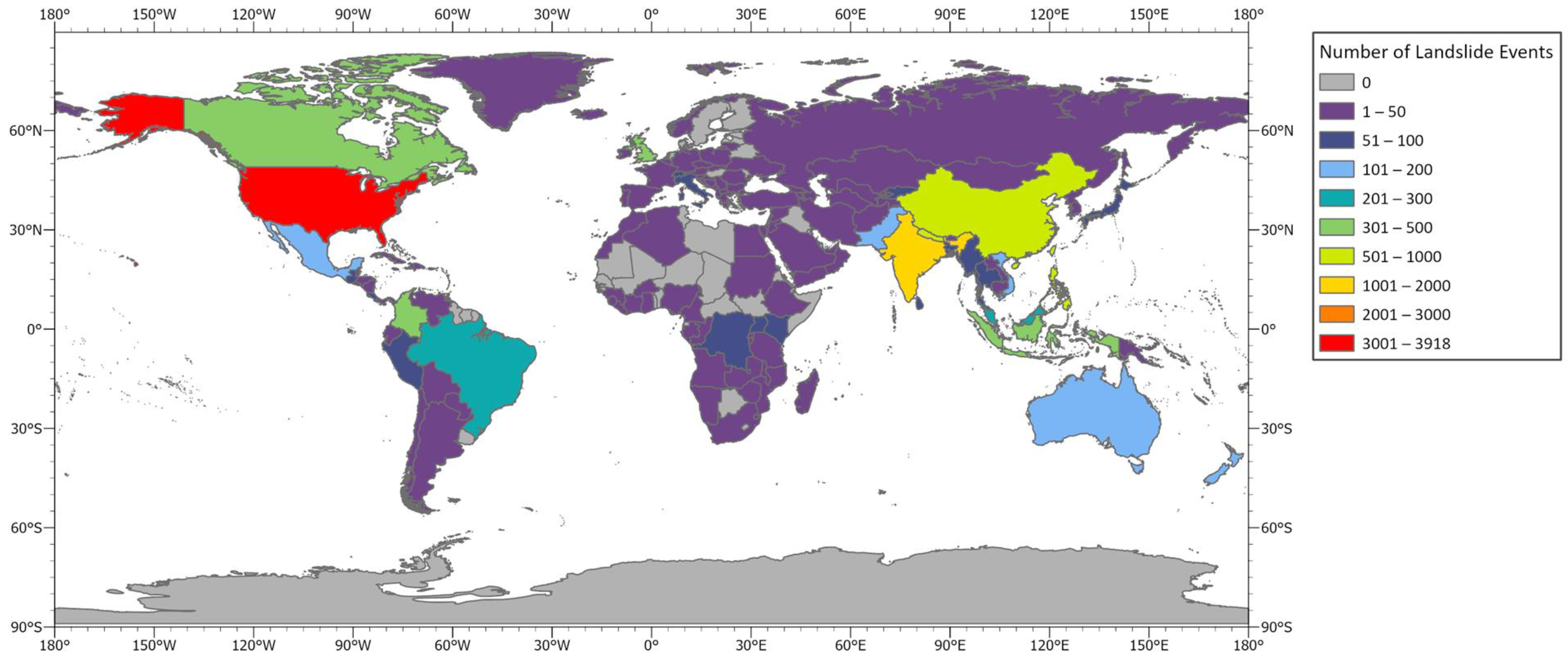
2. Study Area and Landslide Data

As one of the US southeastern coastal states, North Carolina is often impacted by the same Atlantic hurricanes that hit Puerto Rico (such as the case of Hurricane Maria). Because of the likelihood of exposure to Atlantic hurricanes, we are interested in studying the same multi-hazard risks to bridges in North Carolina (NC).

Figure 5a shows the three physiographic regions in North Carolina. North Carolina’s geography is composed of the eastern Coastal Plain Region (see Figure 5d), the central Piedmont (see Figure 5c), and the western Appalachian Mountains (see Figure 5b).

The mountain area (26,572 km²) encompasses the Blue Ridge and the Great Smoky Mountains [19]. The Eastern Continental Divide separates the rivers that flow eastward into the Atlantic Ocean from those flowing westward toward the Tennessee and Ohio rivers [19]. The Coastal Plain (59,363 km²) refers to the low-lying areas extending from the sandy farmland in the east to the Outer Banks, featuring barrier islands and three capes [19]. Last, the Piedmont (43,288 km²), typically described as “the foothills”, is characterized by rolling hills ranging from 90 to 450 m in elevation [19].

Landslides are a common hazard in the western mountains of NC. For example, the 2005 Pigeon River Gorge rockslide event had direct (e.g., road repair, stabilization costs, etc.) and indirect (e.g., interruption of business, commerce, tourism because of lengthy detours, etc.) costs that exceeded 15 million USD [20]. To date, no attempt has been made to discern the probable landslide risks in North Carolina for specific roadway bridge structures.

To evaluate landslide risks, landslide data from 1900 to 2021 were collected from the U.S. Geological Survey (USGS). The NC landslide-prone area is roughly 320 km², and approximately 99.7% of the landslides occurred in the western mountains, with only 0.03% of the landslides occurring in the Piedmont [21]. Belair, Jones [21] developed the US landslide database (version 2.0), and based on the confidence levels, quality of input data, and method used for identification and mapping of each landslide, they suggested a scale system for slope susceptibility to landslides [22]. In their database, the authors recommended that the lowest susceptibility value (1) is for “Possible landslide in the area” and the highest value (8) is for “High confidence in extent or nature of landslide” [22]. In our study, landslide areas with values ranging from 5 (a confident consequential landslide at this location) to 8 were used.

3. Materials and Methods

3.1. Landslide and Bridge Inventory

The landslide inventory used in this study is the USGS dataset [21]. The dataset contains 4794 landslide points and 6653 landslide polygons from 1991 to 2021 (Figure 6). The database is collected and maintained by different agencies and institutions, such as the National Aeronautics and Space Administration (NASA), USGS, and the North Carolina Geological Survey (NCGS).

The bridge inventory for the current study is collected from the North Carolina Department of Transportation (NCDOT) dataset and the Federal Highway Administration (FHWA) dataset. We used the bridge’s ID to combine the two datasets for our analysis. The combined dataset, updated to 2023, contains 22,812 bridges (Figure 7).

3.2. Conditioning Factors

In defining a likely landslide area, we selected several variables known to influence the susceptibility of a slope to fail, including elevation, aspect, slope, rainfall, distance to faults, and distance to rivers for landslides [23,24,25,26,27].

Elevation can significantly affect landslide occurrence; it can also interact with other factors, and their combined effects impact the probability of occurrence [24,28,29]. Elevation data were obtained from the Digital Elevation Model (DEM) provided by the USGS [30] at a resolution of 1 arc-second (Figure 8a). Contour lines that contain elevation values were used to construct a DEM layer with a cell size of 30 m × 30 m [30].

Using DEM, we calculated the aspect variable with the ArcGIS Pro aspect tool (Figure 8b) and the slope variable with the slope tool (Figure 8c). Aspect-related parameters such as exposure to sunlight, drying winds, and discontinuities may influence the occurrence of landslides [25]. Following Ayalew and Yamagishi [31] and Lee and Pradhan [26], we reclassified the aspect variable and divided the aspect into nine classes: flat (−1°), north (0–22.5° and 337.5–360°), northeast (22.5–67.5°), east (67.5–112.5°), southeast (112.5–157.5°), south (157.5–202.5°), southwest (202.5–247.5°), northwest (247.5–292.5°), and west (292.5–337.5°). Based on the order of the classes, we assigned aspect values from 1 to 9 to each class. Aspect value is especially critical to the landslide susceptibility of steep slopes.

High rainfall amounts typically result in high hazard index values for landslides [23]. Rainfall totals were calculated using observation data from the National Oceanic and Atmospheric Administration (NOAA) and the Inverse Distance Weighted (IDW) tool in ArcGIS Pro (Figure 8d).

It is important to recognize that several of the geological, geomorphological, and hydrological factors are implied in the aspect variable [31]. As a result, the only other major factor in triggering landslides that needs to be explicitly investigated is seismicity [9]. Therefore, the distance to faults is an important susceptibility criterion [25] (Figure 8e). We used the Euclidean distance tool in ArcGIS Pro to generate distances to faults [32].

Slopes located closer to rivers are generally more vulnerable to landslides due to factors such as increased water infiltration, erosion, and the destabilizing effect of flowing water [33,34]. We used the Euclidean distance tool to generate the distance to the river in ArcGIS Pro. The river data were collected from the USGS national rivers (NHD) database [35].

Figure 9 illustrates the schematic of the workflow for our models and calculations, which will be further explained in the following section.

3.3. Logistic Regression Model

Logistic regression (LR) allows for estimating the relationship between a categorical variable (e.g., occurrence or no occurrence of an extreme event) and its influential factors [36,37]. It is a useful tool to calculate the probability of the occurrence of an event [36,38,39]. Kleinbaum, Dietz [38] described the logistic model as follows:

$$p=\frac{e^z}{1+e^z}=\frac{1}{1+e^{-z}}$$

(1)

where p is the probability of an event occurrence (1: occurrence; 0: no occurrence). Logit z is assumed to be a linear combination of the independent variables and is defined as follows:

$$z={\beta }_0+{\beta }_1{x}_1+{\beta }_2{x}_2+\dots +{\beta }_i{x}_i$$

(2)

where β₀ is the intercept of the model, x_i is the ith variable, and β_i is the coefficient of the variable x_i. We used the random forest tool in RStudio 2021.09.2+382 (open-source statistical software) for the LR modeling and generated the probability map of event occurrence (Equation (1)) in NC in ArcGIS Pro 3.1.2.

The Receiver Operating Characteristic (ROC) curve is a representation of the performance of a binary classification model [40]. Zhang, Lim [41] used an ROC curve to determine the optimal discrimination threshold for predicting event occurrence. The ROC curve is created by plotting the True Positive Rate (TPR) against the False Positive Rate (FPR) for various threshold values of a model’s predicted probabilities [42,43]. Zhang, Lim [41] and Milanović, Marković [43] further used Area Under Curve (AUC) values between 0.5 and 0.7 to indicate poor precision, values between 0.7 and 0.8 to indicate acceptable precision, values between 0.8 and 0.9 to indicate excellent precision, and values higher than 0.9 to indicate outstanding model precision. We used R to fit the LR models and produced the LR results, ROC curve, and AUC values. This model validation approach is used in the current study in LR modeling. These model validation approaches will also be used in random forest (RF) modeling, as explained in the following section.

3.4. Random Forest Model

According to Alzubi, Nayyar [44], Machine Learning (ML) is about making computers modify their actions in order to improve the actions to attain more accuracy, where accuracy is measured in terms of the number of times the chosen actions result in correct values. ML can be defined as a category of artificial intelligence that enables computers to learn and perform tasks that come naturally to humans, such as learning from past experiences [44]. ML techniques have been extensively applied in spatial statistical analyses to predict and model extreme events [45,46,47].

Introduced by Breiman [48], random forest (RF) is a computationally effective ensemble ML method that constructs the combination of many decision trees that can be used to model the spatial distribution of extreme events and has been applied in geomorphological research, susceptibility mapping, and remote sensing data modeling [47,48,49]. RF has strong algorithmic advantages such as rapid processing capability, easy hyper-parameter optimization, and success in achieving high predictive performance [47]. This technique has been applied to spatial regression analyses to predict the likelihood of extreme events occurring in different regions [43,49,50,51]. It has been combined with multiple decision trees to improve the accuracy and robustness of the model [48].

An RF model can deal with a large amount of data, including both categorical and numerical data, and it can account for complex interactions and validate predictions [49]. The data requirement is for data that represent both occurrence and non-occurrence areas [49]. Therefore, we assigned a value of 1 to occurrence landslide points and a value of 0 to non-occurrence landslide points in our dataset [50]. Identifying the areas and sample conditions from GIS spatial locations is straightforward [11]. However, the accuracy of data mining models, often considered a “black box”, should be rigorously tested due to the challenge of defining variable relationships [49]. In our study, it involved splitting the entire dataset into two parts, where 80% of the dataset was used for training and the remaining 20% of the dataset was employed for validation [11,49].

A study by Kim, Lee [11] focused on landslide susceptibility mapping using ML models, specifically RF and boosted tree models. The performance of the models was evaluated using an ROC analysis and AUC values. The results of the study showed that both the RF and boosted tree models performed well in predicting landslide susceptibility, with the RF model outperforming the boosted tree model in terms of accuracy. The study demonstrated the effectiveness of RF, boosted tree models for landslide susceptibility mapping, and emphasized the importance of slope in landslide susceptibility analyses. Chen et al. [6] also tested the performance of RF to quantify landslide susceptibilities and concluded that RF can reach a 95% confidence level with high AUC values [6].

In this study, we used the RStudio 2021.09.2+382 software for the RF modeling and produced an RF result, an out of bag (OOB) error, an accuracy value, an ROC curve, AUC values, and, finally, a map of the probability of landslide event occurrence in NC.

3.5. North Carolina Highway Bridges

In this study, we focused on bridges situated above water with a length greater than 6 m and excluded those bridges over pipes and culverts or those designed as ramps. A significant number of the bridges on the NC highway system are prestressed concrete stringer bridges and steel girder bridges, with very few other bridge types. However, bridge construction materials are not the focus of the current study. The elevation of the bridge plays a crucial role in determining its susceptibility to damage by streams and rivers. Our previous investigation in Puerto Rico revealed that bridges located at the bottom of valleys are particularly vulnerable to multi-hazard risks that include landslide and flooding events. Hence, similar to the bridge in Las Marias (see Figure 4), the combined hazards can lead to bridge washout. Thus, we further identified bridges likely to be affected by landslides and selectively examined those situated in or near the bottom of valleys.

Throughout this research, we employed various tools in ArcGIS Pro to automatically calculate the bridge’s assumed flooding potential (AFP) based on their geographical locations. These tools included the buffer tool, zonal statistics tool, extract multi-values to points tool, split line to points tool, and bearing distance to line tool. We utilized these tools to generate elevation data for both the banks of a bridge and the elevation of the river. Subsequently, these elevation data were incorporated into the bridge’s AFP calculation, defined by the following equation:

$$B_i=\frac{E_{1i}+E_{2i}}{2}-E_{Li}$$

(3)

where B_i represents the bridge’s AFP, i denotes the bridge’s ID, E_1i and E_2i correspond to the elevations of the two sides of the bridge, and E_Li represents the elevation of the river. AFP is different from bridge clearance as it is physically the approximate bridge height (averaged from the two banks) minus the river elevation from DEM at the location of the bridge. Hence, AFP is not the exact bridge height to the water level but the approximate bridge height to the DEM elevation. Ignored are the actual heights from the bridge bottom to the bridge deck surface. We utilized ArcGIS Pro tools to compute the AFP results (Equation (3) and identified bridge locations within valleys in NC.

To identify bridge locations within a valley, we used several criteria, such as AFP value, landform, slope, and elevation difference. The landforms were classified using the “Geomorphon Landforms” tool in ArcGIS Pro, which categorizes calculated geomorphons into common landform types [52]. Jasiewicz and Stepinski [53] studied the classification and mapping of landform elements and described geomorphon as the landscape representation based on elevation differences around a target cell. Comprising 498 geomorphons, their dataset encompassed all conceivable morphological terrain types, encompassing both common landscape elements and rare, unconventional forms found infrequently on natural terrestrial surfaces [53]. The data were then classified into ten common landform types: flat, peak, ridge, shoulder, spur, slope, hollow, footslope, valley, and pit [52,53].

In the current study, the slope values were determined based on the maximum slope degrees (see Section 3.2) within a 30 m search area around the bridge. The elevation differences were calculated from the maximum elevation within the same 30 m search area around the bridge compared to the bridge’s elevation.

4. Results and Discussion

We utilized 9794 sample points for the LR and RF modeling (4794 for historical landslide occurrences and 5000 for no landslide occurrences). In our dataset, we used a random points tool in ArcGIS Pro to generate 5000 points that had no landslide occurrences.

4.1. Statistical Results

The variables of elevation, aspect, slope, rainfall, distance to faults, and distance to rivers were used in our analysis. The results for the LR model are shown in

Table 1. Coefficient values for LR in the case of each predictor variable in a landslide.

Variable	Unit	Aspect (Reclass) Interact Slope	Significance 1
Elevation *	m	2.264 × 10−3	***
Slope	Degree	6.346 × 10−1	***
Rainfall	mm/year	3.399 × 10−3	***
Distance to faults	m	−1.069 × 10−5	***
Distance to rivers	m	1.515 × 10−4	**
Aspect 2		5.706 × 10−1	***
Aspect 3		1.175 × 100	***
Aspect 4		1.362 × 100	***
Aspect 5		9.241 × 10−1	***
Aspect 6		5.366 × 10−1	***
Aspect 7		−1.296 × 10−1	†
Aspect 8		−2.987 × 10−1	*
Slope: Elevation		−3.752 × 10−4	***
Intercept		−5.523 × 100	***

¹ Significance codes: *** p ≤ 0.001; ** p ≤ 0.01; * p ≤ 0.05; † p ≤ 1.

. We used the slope interaction with the elevation model to analyze the landside sample points. The results for the LR model show that the elevation, aspect, rainfall, slope, aspect 2 to aspect 6, and the distance to rivers are considered positive and significant variables. This means that the landslides would occur more frequently in areas where the elevation is higher, the slope is steeper, the rainfall is larger, the location is far away from a river, and the facing slope is north (aspect 2), northeast (aspect 3), east (aspect 4), southeast (aspect 5), or south (aspect 6). On the other hand, distances to faults and slope interaction elevation are negative and significant, meaning that the high occurrence of landslides in the area is closer to the fault lines. In this case, negative slope interaction means that when the slope is steeper, the elevation will be lower. Furthermore, aspect 7 and aspect 8 are both identified as negative, but only aspect 8 is significant. The interpretation is that landslides will not frequently occur where the facing slope is westward (aspect 8). Finally, it is not conclusive if landslides will likely occur on southwest-facing (aspect 7) slopes.

4.2. Validation and Comparison of Models

In

Table 2. Summary of model performances for the LR model and the RF model for landslides.

Models	Evaluation	Value
Logistic Regression	AIC 1	8116.8
	Accuracy	0.763
	Sensitivity	0.7736
	AUC	0.8431
Random Forest	OOB	16.52%
	Accuracy	0.8269
	Sensitivity	0.8592
	AUC	0.9092

¹ AIC: Akaike information criterion.

, the LR model predicts a percentage of 76.3%, which is a measure of how well the model predicts the correct outcome. Further, in a sensitivity analysis, the model identified an accuracy of 77.4%, indicating the percentage of positive model identification. In the case of AIC (Akaike information criteria) values, a lower AIC value indicates a better model fit. In our case, the 8116.8 value is considered high. (Typical reported AIC values are in the range of 200 [54] to 1,000,000 [55].) As mentioned in Section 3.4, the ROC curve and AUC value have been widely used to validate the performance of the RF and LR models [56]. A higher AUC value indicates better model performance, as it can distinguish between positive and negative cases. In our model, the AUC has a reported accuracy of 84.3%, indicating acceptable model performance.

The OOB error estimate with lower values indicates better model performance, suggesting that the model can generalize new data well. The two a priori hyper-parameters can be optimized: the number of trees in the forest (ntree) and the number of variables tested at each node (mtry), with the optimization aimed at minimizing the OOB error and achieving good model performance [50].

In our RF model, the optimized values were 500 for ntree and 3 for mtry, resulting in an OOB error of 16.5%. Our RF model correctly predicted outcomes with an accuracy of 82.7%, meaning that the model accurately predicted the outcomes. In a sensitivity test, the model correctly identified 86%, a measure of how well it identifies true positive cases. A higher AUC value indicated better model performance, with an accuracy of 90.9%, signifying outstanding model performance.

In our research, we compare the LR model and the RF model to select the best-performing model. The choice of the best model often depends on the specific characteristics of the problem and the data at hand [54]. Based on the accuracy value, AUC value, and ROC curve (see Figure 10), the RF model demonstrated superior performance in predicting landslide occurrence. Consequently, we chose the random forest model to generate the probability of a landslide occurrence map.

4.3. Predicted Probabilities and Susceptibility Map

In order to compare with the LR model, we used the trained RF model to generate the probability of a landslide occurrence map and a susceptibility map. We trained the RF model using R to map the predicted probability of landslide occurrence. Figure 11 shows that the red color represents a higher probability of landslide occurrence, yellow indicates a medium probability, and green signifies a low probability. Figure 12 reveals that 47 bridges will likely experience over 50% of the landslide occurrences in the NC mountain region. Landslides are predicted to occur in over 80% of the area around Watauga County, Jackson County, Henderson County, and Polk County.

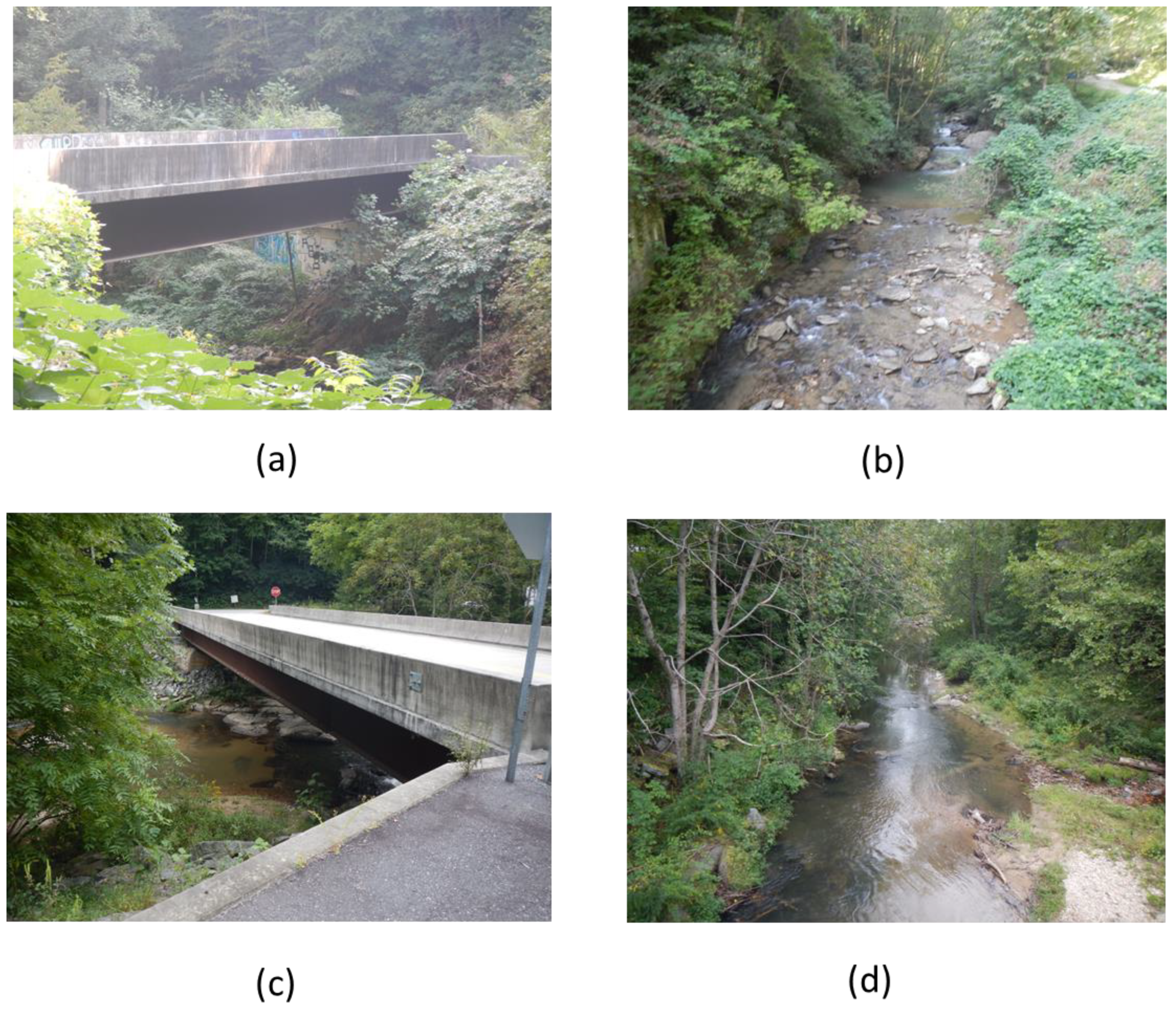
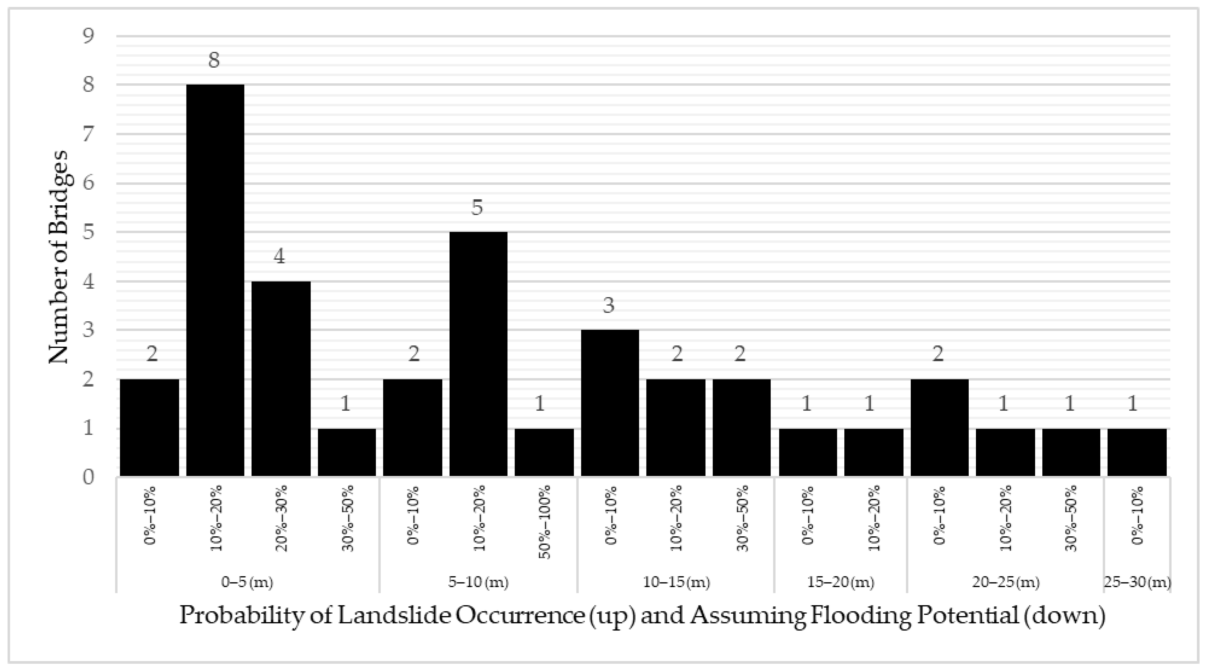
4.4. Bridge in a Valley

After bridge data were retrieved from NCDOT and the FHWA databases, 9462 bridges were identified in North Carolina.

Several of the bridges (see Figure 13, Figure 14, Figure 15, Figure 16 and Figure 17) were visited in September 2023. Figure 13 and Figure 14 showcase bridges situated on ridgetops. Figure 13a,b and Figure 14a,b depict the bridge structure, while Figure 13c,d and Figure 14d illustrate the river bedding. Figure 14c provides a representation of the situation next to the bridge. Despite a high landslide risk (95%), these bridges, built at higher elevations, exhibit a lower susceptibility to landslide impacts. Figure 15a,b, Figure 16a,c, and Figure 17a show the bridge structure, while Figure 15c, Figure 16b,d, and Figure 17b illustrate the circumstances of the river bed. Figure 15 illustrates a bridge constructed at an elevation high above a valley, presenting a 60% probability of landslide occurrence. Figure 16a,b and Figure 17 depict a specific area where several landslides occurred. These two bridges are considered to be bridges at the bottom of valleys in our study. One of these bridges (Bridge ID: 740002) (see Figure 17) has experienced landslides in its vicinity, and slope repair works using soil nails were ongoing during the field visit (see Figure 17c,d).

To establish whether a bridge is in a valley or on a ridge, several criteria were established, including landform (e.g., valley and pit) data, slope (e.g., above 9 degrees), elevation difference (e.g., above 15 m), and AFP value (e.g., under 7 m). The results showed that 21 bridges were in a valley-bottom setting (see Figure 18). It should be noted that AFP can be a misnomer because it does not exactly project the flooding level. Instead, in the current study, AFP is used by assuming that the flooding will reach its full value. Hence, to assess the number of bridges that may be exposed to flooding danger, AFP up to 30 m was applied to the bridge data (see Figure 19).

Finally, we combine the bridge-in-valley data with the probability of landslide occurrence, indicating a bridge’s landslide and flooding risk (see Figure 18 and Figure 19). According to Figure 18, the results showed that three bridges have a lower than 10% chance of landslide occurrence; 12 bridges have a 10% to 20% chance of landslide occurrence; and 5 bridges have a 24% to 32% chance of landslide occurrence. One bridge (ID: 740002) has a 92% chance of landslide occurrence (see Figure 18, red square symbol). Bridge 740002 is a steel stringer/multiple girder bridge with a concrete deck. This bridge was built in 2010, and the last routine inspection of the structure was in September 2021. According to the inspection results, the deck, superstructure, and substructure were still in good condition in 2021.

The risks posed to Bridge 740002 are likely landslides near the bridge foundations as well as upstream and downstream, which may result in increased flood heights from congestion of the channel stream flow during torrential rains. Such multi-hazard analysis has not been previously attempted and should be included in the evaluation of bridges in similar geographical settings. This is especially important in addressing climate extremes, where unprecedented storms are projected for the Carolinas.

Further research was conducted on bridge data in valleys, combined with the probability of landslide occurrence and AFP (see Figure 19 and Appendix A). In Figure 19, the bridges with AFP below 10 m indicate that 23 bridges have a 10% to 20% chance of landslide occurrence, 6 bridges have a 20% to 50% chance of landslide occurrence, and 1 bridge has a 50% to 100% chance of landslide occurrence. Appendix A shows the details of the bridge information, including bridge ID, longitude, latitude, AFP, our assessment (using four criteria for classification), extra observations (confirming the classification method), and the probability of landslide occurrence. When considering AFP, additional field observations were made (see Appendix A), which indicates that bridges with AFP above 7 m and below 30 m are not necessarily located at the bottom of a valley. As observed in Figure 13 and Figure 14, these bridges may be better classified as either bridges at the mid-height of a valley or on a ridgetop. The field observations were used to validate the bridges in valleys in Appendix A, where only Bridge 020021 does not fit our criteria for a bridge in a valley (AFP of less than 7 m). The classification method used in the current study achieved a 97% accuracy rate in the bridge-in-valley selection.

5. Conclusions

The 2018 Hurricane Maria resulted in more than 40,000 landslides and damaged 388 bridges in Puerto Rico. A close examination of several of the damaged bridges revealed the danger of multi-hazard risks (landslide + flooding) for bridges in valleys. North Carolina, on the east coast of the U.S., is also exposed to the impacts of seasonal Atlantic hurricanes. Hence, to investigate similar risks to bridges in North Carolina, a landslide risk susceptibility analysis has been conducted. In this study, we identified that the majority of landslides occur in the mountainous region of North Carolina, thus posing a potential threat to numerous bridges in that region.

Using logistic regression (LR) and random forest (RF) modeling, a landslide risk susceptibility map was created. Conditioning factors included in the current study are aspect variables and seismicity (distance to faults). The geomorphic, geological, and hydrological considerations are inclusive of the aspect variables of the conditioning factors. The results from the two models have accuracy rates of 76.3% and 82.7% for the LR and RF models, respectively. Using the ROC curves, the RF model is also shown to be more sensitive than the LR model in predicting landslide risks. Combining highway and roadway bridge data, bridges with high landslide risk are then identified.

Further analysis using landform data and bridge assumed flooding potential (AFP) helped identify bridges in valleys. The results showed 37 bridges exposed to both landslide and flooding risks. One particular bridge (ID: 740002) has been found to be exposed to high landslide and flooding risks. Observations from a field visit indicated that ongoing construction efforts have been carried out to address localized landslides near the bridge location. This confirmed our analysis result (see Figure 18, red square symbol), and the observations on Bridge 740002 (see Figure 17) align with our findings, indicating the potential exposure to multi-hazard (landslide with flooding) dangers. This observation reinforced our confidence that the landslide risk map is accurate and can serve as a valuable tool for managers and decision-makers, enabling proactive measures to prevent potential bridge damage in the future.

The development of a landslide risk prediction model poses a challenge if we take into consideration the complex nature of geo-environments, encompassing factors such as geology, hydrology, topography, and human activities (land use) [4]. The current study covered a large area and only considered the aspect variable and seismicity; hence, future work aiming for increased precision can delve into additional factors such as geology and lithology.

The current study used bridge AFP as an indicator of the potential for combined landslide and flooding risks. If the flooding level reaches AFP, then the uplift forces from the rapid channel flow may lift the bridge deck and result in a bridge washout. Future work will extend the analysis of flooding risk and the connection to landslides, which can further predict the scour potential that poses an additional threat to bridges. The addition of flooding risks would provide managers and decision-makers with more complete information to act preemptively to prevent damage to bridges.

References

1. Regmi, N.R.; Giardino, J.R.; McDonald, E.V.; Vitek, J.D. A comparison of logistic regression-based models of susceptibility to landslides in western Colorado, USA. Landslides 2014, 11, 247–262. [Google Scholar] [CrossRef]
2. Sun, D.; Wen, H.; Zhang, Y.; Xue, M. An optimal sample selection-based logistic regression model of slope physical resistance against rainfall-induced landslide. Nat. Hazards 2021, 105, 1255–1279. [Google Scholar] [CrossRef]
3. Pourghasemi, H.R.; Teimoori Yansari, Z.; Panagos, P.; Pradhan, B. Analysis and evaluation of landslide susceptibility: A review on articles published during 2005–2016 (periods of 2005–2012 and 2013–2016). Arab. J. Geosci. 2018, 11, 193. [Google Scholar] [CrossRef]
4. Kirschbaum, D.B.; Adler, R.; Hong, Y.; Hill, S.; Lerner-Lam, A. A global landslide catalog for hazard applications: Method, results, and limitations. Nat. Hazards 2010, 52, 561–575. [Google Scholar] [CrossRef]
5. Kirschbaum, D.; Stanley, T.; Zhou, Y. Spatial and temporal analysis of a global landslide catalog. Geomorphology 2015, 249, 4–15. [Google Scholar] [CrossRef]
6. Chen, W.; Zhang, S.; Li, R.; Shahabi, H. Performance evaluation of the GIS-based data mining techniques of best-first decision tree, random forest, and naïve Bayes tree for landslide susceptibility modeling. Sci. Total Environ. 2018, 644, 1006–1018. [Google Scholar] [CrossRef]
7. Nhu, V.H.; Shirzadi, A.; Shahabi, H.; Singh, S.K.; Al-Ansari, N.; Clague, J.J.; Jaafari, A.; Chen, W.; Miraki, S.; Dou, J.; et al. Shallow Landslide Susceptibility Mapping: A Comparison between Logistic Model Tree, Logistic Regression, Naïve Bayes Tree, Artificial Neural Network, and Support Vector Machine Algorithms. Int. J. Environ. Res. Public Health 2020, 17, 2749. [Google Scholar] [CrossRef] [PubMed]
8. Wubalem, A.; Meten, M. Landslide susceptibility mapping using information value and logistic regression models in Goncha Siso Eneses area, northwestern Ethiopia. SN Appl. Sci. 2020, 2, 807. [Google Scholar] [CrossRef]
9. Ganga, A.; Elia, M.; D’Ambrosio, E.; Tripaldi, S.; Capra, G.F.; Gentile, F.; Sanesi, G. Assessing Landslide Susceptibility by Coupling Spatial Data Analysis and Logistic Model. Sustainability 2022, 14, 8426. [Google Scholar] [CrossRef]
10. USGS. Landslides 101. Available online: https://www.usgs.gov/programs/landslide-hazards/landslides-101 (accessed on 30 August 2023).
11. Kim, J.-C.; Lee, S.; Jung, H.-S.; Lee, S. Landslide susceptibility mapping using random forest and boosted tree models in Pyeong-Chang, Korea. Geocarto Int. 2018, 33, 1000–1015. [Google Scholar] [CrossRef]
12. Highland, L.M.; Bobrowsky, P. The Landslide Handbook-A Guide to Understanding Landslides; US Geological Survey: Reston, VA, USA, 2008.
13. Ozturk, D.; Uzel-Gunini, N. Investigation of the effects of hybrid modeling approaches, factor standardization, and categorical mapping on the performance of landslide susceptibility mapping in Van, Turkey. Nat. Hazards 2022, 114, 2571–2604. [Google Scholar] [CrossRef]
14. Bessette-Kirton, E.K.; Cerovski-Darriau, C.; Schulz, W.H.; Coe, J.A.; Kean, J.W.; Godt, J.W.; Thomas, M.A.; Hughes, K.S. Landslides triggered by Hurricane Maria: Assessment of an extreme event in Puerto Rico. GSA Today 2019, 29, 4–10. [Google Scholar]
15. Ortiz, F. Coming Back from Disaster. Public Roads 2020, 83, FHWA-HRT-20-002. [Google Scholar]
16. Keellings, D.; Hernández Ayala, J.J. Extreme Rainfall Associated With Hurricane Maria Over Puerto Rico and Its Connections to Climate Variability and Change. Geophys. Res. Lett. 2019, 46, 2964–2973. [Google Scholar] [CrossRef]
17. Miele, P.; Di Napoli, M.; Guerriero, L.; Ramondini, M.; Sellers, C.; Annibali Corona, M.; Di Martire, D. Landslide Awareness System (LAwS) to Increase the Resilience and Safety of Transport Infrastructure: The Case Study of Pan-American Highway (Cuenca–Ecuador). Remote Sens. 2021, 13, 1564. [Google Scholar] [CrossRef]
18. Schlögl, M.; Richter, G.; Avian, M.; Thaler, T.; Heiss, G.; Lenz, G.; Fuchs, S. On the nexus between landslide susceptibility and transport infrastructure—An agent-based approach. Nat. Hazards Earth Syst. Sci. 2019, 19, 201–219. [Google Scholar] [CrossRef]
19. North Carolina Secretary of State Kids Page Geography. Geography. Available online: https://www.sosnc.gov/divisions/publications/kids_page_geography (accessed on 20 June 2023).
20. NCGS. Introduction to Landslides in North Carolina. Available online: https://www.deq.nc.gov/about/divisions/energy-mineral-and-land-resources/north-carolina-geological-survey/geologic-hazards/landslides (accessed on 30 August 2023).
21. Belair, G.M.; Jones, E.S.; Slaughter, S.L.; Mirus, B.B. Landslide Inventories across the United States Version 2: U.S. Geological Survey Data Release; USGS, Ed.; US Geological Survey: Reston, VA, USA, 2022.
22. Mirus, B.B.; Jones, E.S.; Baum, R.L.; Godt, J.W.; Slaughter, S.; Crawford, M.M.; Lancaster, J.; Stanley, T.; Kirschbaum, D.B.; Burns, W.J.; et al. Landslides across the USA: Occurrence, susceptibility, and data limitations. Landslides 2020, 17, 2271–2285. [Google Scholar] [CrossRef]
23. Abella, E.A.C.; Van Westen, C.J. Generation of a landslide risk index map for Cuba using spatial multi-criteria evaluation. Landslides 2007, 4, 311–325. [Google Scholar] [CrossRef]
24. Chau, K.T.; Chan, J.E. Regional bias of landslide data in generating susceptibility maps using logistic regression: Case of Hong Kong Island. Landslides 2005, 2, 280–290. [Google Scholar] [CrossRef]
25. Feizizadeh, B.; Blaschke, T.; Nazmfar, H.; Rezaei Moghaddam, M.H. Landslide Susceptibility Mapping for the Urmia Lake basin, Iran: A multi- Criteria Evaluation Approach using GIS. Int. J. Environ. Res. 2013, 7, 319–336. [Google Scholar]
26. Lee, S.; Pradhan, B. Landslide hazard mapping at Selangor, Malaysia using frequency ratio and logistic regression models. Landslides 2007, 4, 33–41. [Google Scholar] [CrossRef]
27. Mondini, A.C. Measures of Spatial Autocorrelation Changes in Multitemporal SAR Images for Event Landslides Detection. Remote Sens. 2017, 9, 554. [Google Scholar] [CrossRef]
28. Dai, F.C.; Lee, C.F. Landslide characteristics and slope instability modeling using GIS, Lantau Island, Hong Kong. Geomorphology 2002, 42, 213–228. [Google Scholar] [CrossRef]
29. Mousavi, S.Z.; Kavian, A.; Soleimani, K.; Mousavi, S.R.; Shirzadi, A. GIS-based spatial prediction of landslide susceptibility using logistic regression model. Geomat. Nat. Hazards Risk 2011, 2, 33–50. [Google Scholar] [CrossRef]
30. USGS. 1 Arc-Second Digital Elevation Models (DEMs)—USGS National Map 3DEP Downloadable Data Collection; US Geological Survey: Reston, VA, USA, 2023.
31. Ayalew, L.; Yamagishi, H. The application of GIS-based logistic regression for landslide susceptibility mapping in the Kakuda-Yahiko Mountains, Central Japan. Geomorphology 2005, 65, 15–31. [Google Scholar] [CrossRef]
32. NCDEQ. Geologic Faults; NCDEQ: Raleigh, NC, USA, 2022.
33. Cebulski, J. Impact of river erosion on variances in colluvial movement and type for landslides in the Polish Outer Carpathians. Catena 2022, 217, 106415. [Google Scholar] [CrossRef]
34. Gómez, H.; Kavzoglu, T. Assessment of shallow landslide susceptibility using artificial neural networks in Jabonosa River Basin, Venezuela. Eng. Geol. 2005, 78, 11–27. [Google Scholar] [CrossRef]
35. USGS. USGS National Hydrography Dataset Best Resolution (NHD)—North Carolina (Published 20230305) Shapefile; US Geological Survey: Reston, VA, USA, 2023.
36. Bai, S.-B.; Wang, J.; Lü, G.-N.; Zhou, P.-G.; Hou, S.-S.; Xu, S.-N. GIS-based logistic regression for landslide susceptibility mapping of the Zhongxian segment in the Three Gorges area, China. Geomorphology 2010, 115, 23–31. [Google Scholar] [CrossRef]
37. VanderWeele, T.J.; Knol, M.J. A tutorial on interaction. Epidemiol. Methods 2014, 3, 33–72. [Google Scholar] [CrossRef]
38. Kleinbaum, D.G.; Dietz, K.; Gail, M.; Klein, M.; Klein, M. Logistic Regression; Springer: Berlin/Heidelberg, Germany, 2002. [Google Scholar]
39. Budimir, M.E.A.; Atkinson, P.M.; Lewis, H.G. A systematic review of landslide probability mapping using logistic regression. Landslides 2015, 12, 419–436. [Google Scholar] [CrossRef]
40. Nahm, F.S. Receiver operating characteristic curve: Overview and practical use for clinicians. Korean J. Anesthesiol. 2022, 75, 25–36. [Google Scholar] [CrossRef]
41. Zhang, Y.; Lim, S.; Sharples, J.J. Modelling spatial patterns of wildfire occurrence in South-Eastern Australia. Geomat. Nat. Hazards Risk 2016, 7, 1800–1815. [Google Scholar] [CrossRef]
42. Park, S.H.; Goo, J.M.; Jo, C.H. Receiver operating characteristic (ROC) curve: Practical review for radiologists. Korean J. Radiol. 2004, 5, 11–18. [Google Scholar] [CrossRef]
43. Milanović, S.; Marković, N.; Pamučar, D.; Gigović, L.; Kostić, P.; Milanović, S.D. Forest Fire Probability Mapping in Eastern Serbia: Logistic Regression versus Random Forest Method. Forests 2021, 12, 5. [Google Scholar] [CrossRef]
44. Alzubi, J.; Nayyar, A.; Kumar, A. Machine Learning from Theory to Algorithms: An Overview. J. Phys. Conf. Ser. 2018, 1142, 012012. [Google Scholar] [CrossRef]
45. Chen, W.; Peng, J.; Hong, H.; Shahabi, H.; Pradhan, B.; Liu, J.; Zhu, A.-X.; Pei, X.; Duan, Z. Landslide susceptibility modelling using GIS-based machine learning techniques for Chongren County, Jiangxi Province, China. Sci. Total Environ. 2018, 626, 1121–1135. [Google Scholar] [CrossRef] [PubMed]
46. Jain, P.; Coogan, S.C.P.; Subramanian, S.G.; Crowley, M.; Taylor, S.; Flannigan, M.D. A review of machine learning applications in wildfire science and management. Environ. Rev. 2020, 28, 478–505. [Google Scholar] [CrossRef]
47. Kavzoglu, T.; Teke, A. Predictive Performances of Ensemble Machine Learning Algorithms in Landslide Susceptibility Mapping Using Random Forest, Extreme Gradient Boosting (XGBoost) and Natural Gradient Boosting (NGBoost). Arab. J. Sci. Eng. 2022, 47, 7367–7385. [Google Scholar] [CrossRef]
48. Breiman, L. Random Forests. Mach. Learn. 2001, 45, 5–32. [Google Scholar] [CrossRef]
49. Taalab, K.; Cheng, T.; Zhang, Y. Mapping landslide susceptibility and types using Random Forest. Big Earth Data 2018, 2, 159–178. [Google Scholar] [CrossRef]
50. Park, S.; Kim, J. Landslide Susceptibility Mapping Based on Random Forest and Boosted Regression Tree Models, and a Comparison of Their Performance. Appl. Sci. 2019, 9, 942. [Google Scholar] [CrossRef]
51. Chen, W.; Xie, X.; Wang, J.; Pradhan, B.; Hong, H.; Bui, D.T.; Duan, Z.; Ma, J. A comparative study of logistic model tree, random forest, and classification and regression tree models for spatial prediction of landslide susceptibility. Catena 2017, 151, 147–160. [Google Scholar] [CrossRef]
52. ESRI. Geomorphon Landforms (Spatial Analyst). Available online: https://pro.arcgis.com/en/pro-app/3.1/tool-reference/spatial-analyst/geomorphon-landforms.htm (accessed on 24 November 2023).
53. Jasiewicz, J.; Stepinski, T.F. Geomorphons—A pattern recognition approach to classification and mapping of landforms. Geomorphology 2013, 182, 147–156. [Google Scholar] [CrossRef]
54. Quesada-Román, A. Landslide risk index map at the municipal scale for Costa Rica. Int. J. Disaster Risk Reduct. 2021, 56, 102144. [Google Scholar] [CrossRef]
55. Nowicki Jessee, M.; Hamburger, M.W.; Allstadt, K.; Wald, D.J.; Robeson, S.M.; Tanyas, H.; Hearne, M.; Thompson, E.M. A global empirical model for near-real-time assessment of seismically induced landslides. J. Geophys. Res. Earth Surf. 2018, 123, 1835–1859. [Google Scholar] [CrossRef]
56. Chen, W.; Sun, Z.; Han, J. Landslide Susceptibility Modeling Using Integrated Ensemble Weights of Evidence with Logistic Regression and Random Forest Models. Appl. Sci. 2019, 9, 171. [Google Scholar] [CrossRef]
Figure 1. Number of landslide events from 2007 to 2023 by country (generated from NASA data).
Geohazards 05 00015 g001
Figure 2. Landslide in Puerto Rico after 2017 Hurricane Maria: surface observations indicated rotational slope failures with debris flows. (a) coastal sand flow, (b) earth flow with high silt content, (c) multiple slides, and (d) smoothed slide. (Bedrock is mostly volcaniclastic sandstone and siltstone of Yauco formation, and soils are Maricao Ultisols.) (Photo credit: Shen-En Chen).
Geohazards 05 00015 g002
Figure 3. Landslide in Puerto Rico after 2017 Hurricane Maria: surface observations indicated failure of rocky slopes. (Bedrock is mostly serpentinite, chert, and calcareous sandstone.) (a) debris flow with exposed bedrock, (b) slope with rock fragments and (c) rockslide with significant fines. (Photo credit: Shen-En Chen).
Geohazards 05 00015 g003
Figure 4. A new bridge under construction in Las Marias—heavy flooding resulted in localized landslides and the washout of the original bridge. (a) bridge serving trapped residences, (b) bridge embankment with debris from upstream landslides, (c) scoured embankment, and (d) newly repaired bridge approach. (Photo credit: Shen-En Chen).
Geohazards 05 00015 g004
Figure 5. Study area with location map illustrating North Carolina’s three distinct physiographic regions. (a) North Carolina distinct physiographic region distribution, (b) Blue Ridge Mountain area, (c) Piedmont area, and (d) Coastal Plain area.
Geohazards 05 00015 g005
Figure 6. Location of landslide points and polygons within the study area. (a) Showing closer version in Ashe County, Watauga County, and Avery County. (b) Showing NC statewide results and closer version location (red square) in NC.
Geohazards 05 00015 g006
Figure 7. Location of bridges within the study area.
Geohazards 05 00015 g007
Figure 8. Landslide conditioning factors used in this study: (a) Elevation, (b) Aspect, (c) Slope, (d) Rainfall, (e) Distance to fault, (f) Distance to river.
Geohazards 05 00015 g008
Figure 9. A schematic of the calculation workflow for the probability of landslide occurrence map and bridges in the valley.
Geohazards 05 00015 g009
Figure 10. ROC curves of the LR model and the RF model.
Geohazards 05 00015 g010
Figure 11. Landslide risk map in North Carolina.
Geohazards 05 00015 g011
Figure 12. Bridges with a landslide risk map in NC’s mountain area. Showing the bridges with a 50% or greater probability of being impacted by a landslide.
Geohazards 05 00015 g012
Figure 13. Example of a bridge on a ridgetop (Bridge ID: 440375, a steel girder bridge). (a) Bridge’s side face, (b) Bridge’s girder, (c) Riverbed, and (d) Riverbank. (Photo credit: Shen-En Chen and Sophia Lin).
Geohazards 05 00015 g013
Figure 14. Example of a bridge sufficiently higher than the valley region (Bridge ID: 740031, a prestressed concrete stringer bridge). (a) Bridge’s side face, (b) Bridge’s surface, (c) Riverbank, and (d) Riverbed. (Photo credit: Shen-En Chen and Sophia Lin).
Geohazards 05 00015 g014
Figure 15. Example of bridges in valleys (Bridge ID: 740027, a steel girder bridge). (a) Bridge’s side face, (b) Bridge’s girder, and (c) Riverbed. (Photo credit: Shen-En Chen and Sophia Lin).
Geohazards 05 00015 g015
Figure 16. Examples of bridges in valleys (Bridge ID: 100653, a steel girder bridge). (a) Bridge’s side face, (b) Riverbed, (c) Bridge’s side face, and (d) Riverbed. (Photo credit: Shen-En Chen and Sophia Lin).
Geohazards 05 00015 g016
Figure 17. Example of a valley bridge near a landslide with visible debris flow and rockslide (Bridge ID: 740002, a prestressed concrete stringer bridge). (a) Bridge’s side face, (b) Riverbed, (c) Riverbank infrastructure, and (d) Landslide around bridge. (Photo credit: Shen-En Chen and Sophia Lin).
Geohazards 05 00015 g017
Figure 18. Bridges in a valley under 7 m above stream elevation, assuming flooding potential (AFP) in NC’s mountain area and indicating the potential for exposure to multi-hazard (landslide with flooding) dangers.
Geohazards 05 00015 g018
Figure 19. Probability of landslide occurrence combined with AFP.
Geohazards 05 00015 g019