Article

Non-Stationary Flood Discharge Frequency Analysis in West Africa

by
Aymar Yaovi Bossa
1,*,
Jean de Dieu Akpaca
1,
Jean Hounkpè
1,*,
Yacouba Yira
2 and
Djigbo Félicien Badou
3
1
National Institute of Water, University of Abomey-Calavi, P.O. Box 526, Cotonou 01, Benin
2
Applied Science and Technology Research Institute (IRSAT/CNRST), Ouagadougou P.O. Box 7047, Burkina Faso
3
Laboratoire des Sciences Végétales, Horticoles, et Forestières, Université Nationale d’Agriculture, Kétou BP 5, Benin
*
Authors to whom correspondence should be addressed.
GeoHazards 2023, 4(3), 316-327; https://doi.org/10.3390/geohazards4030018
Submission received: 12 June 2023 / Revised: 1 August 2023 / Accepted: 8 August 2023 / Published: 11 August 2023

Abstract

:
With climate change and intensification of the hydrological cycle, the stationarity of hydrological variables is becoming questionable, requiring appropriate flood assessment models. Frequency analysis is widely used for flood forecasting. This study aims to determine the most suitable models (stationary and non-stationary) for estimating the maximum flows observed at some stations spread across West Africa. A statistical analysis of the annual maximum flows in terms of homogeneity, stationarity, and independence was carried out through the Pettitt, modified Mann–Kendall, and Wald–Wolfowitz tests, respectively, to identify the stations whose flows are non-stationary. After that, the best-correlated climate covariates with the annual maximum flows of the non-stationary stations were determined. The covariates explored are the climatic indices of sea surface temperatures (SST). Finally, different non-stationary GEV models were derived by varying the scale and position parameters of the best-correlated index for each station. The results indicate that 56% of the annual maximum flow series are non-stationary. As per the Bayes information criterion (BIC) values, the performance of the non-stationary models (GEV, generalized extreme values) is largely greater than that of the stationary models. These good performances of non-stationary models using climatic indices open perspectives for the prediction of extreme flows in the study area.

1. Introduction

Controlling rainfall extremes is a major challenge of our century. Every year, these extremes cause damage in the world in general and in West Africa in particular. The damage to the socio-economic level is very important as evidenced by several reports such as that of the post-disaster needs assessment produced by the National Agency for Civil Protection (ANPC) of Benin, which indicates that in 2010, floods caused about fifty-three billion two hundred and ninety-five million (53,295,000,000) XOF in losses, 27 deaths, 317,576 people affected, and many hectares of crops washed away [1]. Following the evolution of these extremes under the influence of factors such as climate change, one would expect more frequent events in the future. Frequency analysis is a privileged tool for predicting extreme floods. It consists of studying past events, characterizing a given hydrological process, in order to define the probabilities of future appearance.
In several frequency analysis studies, non-stationarity has not been considered [2,3,4,5,6] mainly in West Africa. However, with global changes including climate change, several authors have indicated that stationarity is “dead” [7]. Very few studies have examined the non-stationary issues in West Africa [8] while there has been an effort of exploring the non-stationarity in flood frequency in South Africa [9] and other parts of the world [10,11,12,13,14,15]. For instance, Hounkpè et al. [8] made a non-stationary frequency study of flows in the Ouémé basin in West Africa. To our knowledge, there are no studies focused on non-stationary frequency analysis on the scale of West Africa. Detecting the presence and attributing the source of non-stationarity in hydroclimatic extremes is vital to understanding and managing water resources in a changing world [16]. It is, therefore, necessary to take into account non-stationarity in the data in any frequency analysis.
Non-stationary flood frequency analysis is performed when the assumption of stationarity in hydrologic extremes values used for infrastructure design and others (independent and identically distributed time series of extreme flow data) is no longer valid. This implies that the process of flood generation may depend on other variables (named covariates) such as time, climate indexes, and soil moisture. By taking into account these covariates, many authors have improved the performance of flood frequency analysis [8,10,11,12,13,14,15]. Considering a stationary distribution for analyzing a non-stationary variable would necessarily increase the uncertainties in the frequency analysis. Some causes of non-stationarity in recorded data include climate change, land use change, and anthropic activities.
Non-stationary frequency analysis takes into account covariates representing spatial and temporal non-stationarities in the data. Several covariates—whether climatic or hydrological—can be explored to develop better frequency models. This study aims to develop non-stationary flood frequency models of the annual maximum flows of major rivers in West Africa for future exploration of flood forecasting. Specifically, it will evaluate the homogeneity, stationarity, and independence of the maximum annual flow data of the study area; explore possible climatic covariates for annual maximum flows indicating non-stationarity; and perform non-stationary flood frequency analysis for stations with good correlation with climate covariates for hydrological forecasting. This study is among the first of its kinds to perform the non-stationary flood frequency analysis on the scale of West Africa by exploring many climate indexes that could be correlated with the annual maximal discharge data across the study area.

2. Materials and Methods

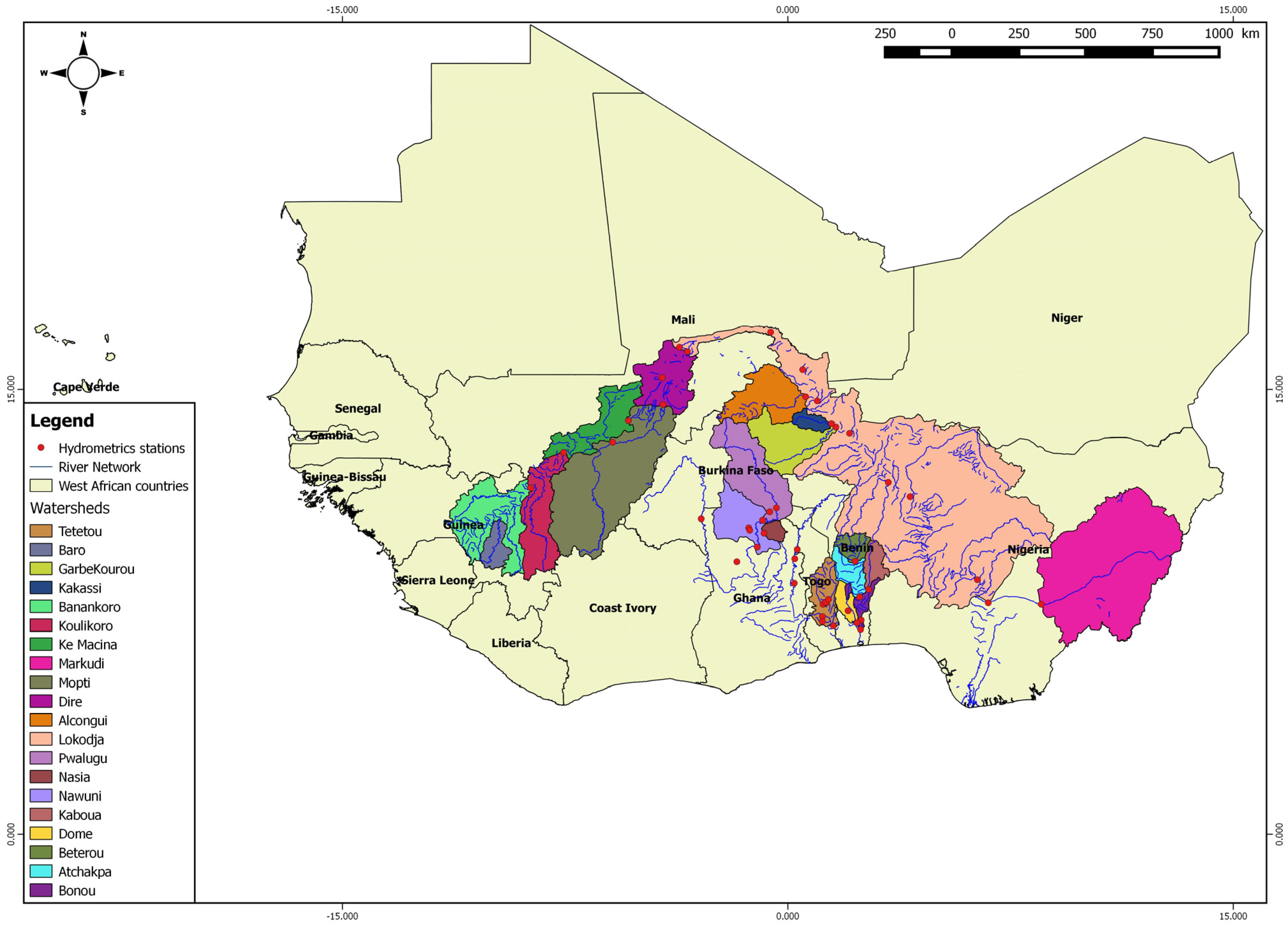
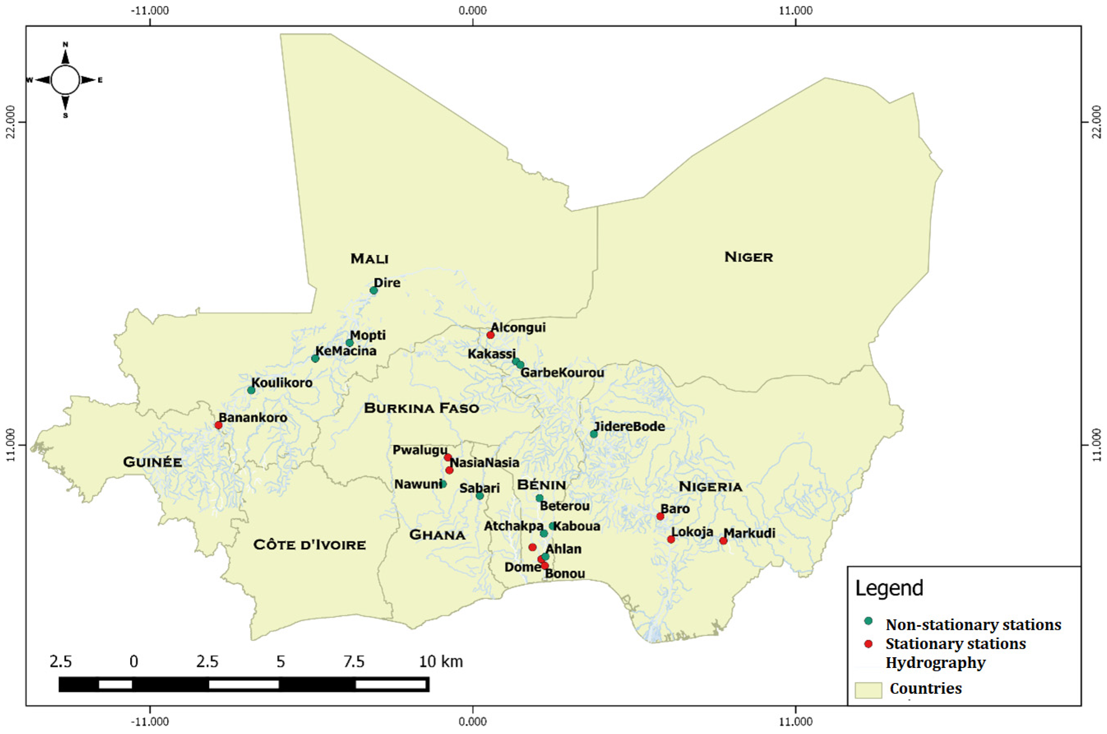
2.1. Description of the Study Area

West Africa has wet and dry seasons resulting from the interaction of two migrating air masses. Where these two air masses meet is a belt of varying width and stability called the Intertropical Convergence Zone (ITCZ) [17]. The northern and southern migrations of the ITCZ, which follows the apparent movement of the sun, control the climate of the region.
The lowland climates of West Africa are characterized by uniformly high sunshine and high temperatures throughout the year with annual means usually above 18 °C. In the Sahel, maximum temperatures can reach above 40 °C [18]. Not only scarcity of rainfall but also its variability and unpredictability become more significant with latitude [18].
Other features of West Africa’s rainfall include frequent and short-term heavy rains that cause severe soil erosion, particularly on cleared and bare croplands; the emergence of a bimodal rainfall belt at some distance inland from the coast to eastern Sierra Leone to Nigeria, and the variability in the amount, timing, duration, and cessation increasing from the wettest to the driest areas. In coastal areas, the percentage of annual variability varies from 10 to 20 percent, while near the Sahara in the Sahel, it can exceed 40 percent. Three (03) climatic zones are observed in the region [19]:
-
The arid zone or Sahel Zone includes the Sahel or the Sahelian zone and has up to 750 mm of rainfall in a single short rainy season with an extended dry season of up to 10 months. The dry season sometimes extends into years causing severe droughts. This area includes parts of northern Senegal, parts of Mali, Burkina Faso, and Niger.
-
The semi-arid zone or Guinea Savanna Zone includes approximately the southern Sahel and covers the southern parts of Mali, Burkina Faso, Niger, Chad and the upper parts of Guinea-Bissau, Guinea, Togo, northern Benin, Nigeria, Cameroon, and the Central African Republic. The average annual rainfall, from 750 mm to 1250 mm, falls in one season followed by a 7- to 8-months-long dry season.
-
The subhumid zone or Equatorial Forest Zone includes southern Guinea-Bissau, the upper parts of Guinea, the southernmost parts of Mali and Burkina Faso and the southern parts of Ghana, Côte d’Ivoire, Cameroon, Sierra Leone, Benin, and the central parts of Nigeria. The average annual rainfall is between 1250 mm and 1500 mm in one season.
River basins as well as the stations considered in this study are displayed in Figure 1.

2.2. Data Collected

The discharge data of forty-six (46) stations in West African countries were obtained through the Global Runoff Data Center [20]. These data were available from 1948 to 2013 for most stations. However, the period between 1948 and 1979 has a large number of missing data. The SST climate indices were downloaded on 1 September 2021, as indicated below:
-
Tropical North Atlantic Index (TNAI) and TSAI (Tropical South Atlantic Index): These two indices are located in the tropical Atlantic. TNAI SSTs range from 5.5° N/23.5° N–15° W/57.5° W and TSAI from 0/20° S–10° E/30° W. These data are from the NOAA CPC archives [21]. These data downloaded are from 1948 to 2020 and are available on www.esrl.noaa.gov/psd/data/correlation/tna.data (accessed on 1 September 2021) and www.esrl.noaa.gov/psd/data/correlation/tsa.data (accessed on 1 September 2021).
-
Dipole Mode Index East (DMIE): The DMIE is located in the Indian Ocean in the range 10 S–10 N, 50 E–70 E [22]. These downloaded data are from 1870 to 2020 on https://psl.noaa.gov/gcos_wgsp/Timeseries/Data/dmieast.had.long.data (accessed on 1 September 2021).
-
Dipole Mode Index West (DMIW): The DMIW is located in the Indian Ocean in the range 10 S: 0.90 E–110 E [22]. These data downloaded are from 1870 to 2020 on https://psl.noaa.gov/gcos_wgsp/Timeseries/Data/dmiwest.had.long.data (accessed on 1 September 2021).
-
Dipole Mode Index (DMI): The DMI is calculated from the difference between the two East and Ouest indices located in the Indian Ocean [22]. The SSTs of the DMI are between the difference 10 S: 10 N, 50 E–70 E and 10 S: 0.90 E–110 E. It is available on https://psl.noaa.gov/gcos_wgsp/Timeseries/Data/dmi.had.long.data (accessed on 1 September 2021). These data downloaded are from 1870 to 2020.
-
MEI (Multivariate ENSO Index): It is calculated from the values of the six variables (surface pressure, zonal and meridian component of the surface wind, sea surface temperature, surface air temperature and cloud cover) [23]. Available on https://www.psl.noaa.gov/enso/mei (accessed on 1 September 2021), the MEI is part of the Pacific Ocean indices. This is a bimonthly index; these downloaded data are from 1979 to 2020.
-
ONI (Oceanic Nino Index): obtained on https://origin.cpc.ncep.noaa.gov/products/analysis_monitoring/ensostuff/ONI_v5.php (accessed on 1 September 2021), this index is also part of the indices of the Pacific Ocean [21]. This trimonthly index was downloaded from 1950 to 2020.

2.3. Methods

2.3.1. Data Quality Assessment

For the construction of a good-quality data series, the following steps were considered:
-
delete stations with less than thirty (30) years of data available from at least 1980 to recent period.
-
determine the maximum flow values for each year at each station: the maximum per block (per year) approach is adopted [24]
-
delete the years whose maximum discharge value does not fall within the peak of rainy season (between June and November).
-
remove stations having less than twenty (20) years of continuous data.
-
remove outliers of annual maximum data obtained via the boxplot. By comparing the maximum values with the limit value corresponding to the station for the corresponding boxplot, we eliminated those below the limit value.

2.3.2. Data Processing

Verification of data consistency, stationarity, and independence: The Pettitt test [25], a nonparametric test, was used to test a shift in the central tendency of time series. The null hypothesis H0 of no change is tested against the alternative hypothesis HA of a change at the significance level of 5%. The modified Mann–Kendall test [26] was used to test the stationarity of the data while the Wald–Wolfowitz Independence test [27] was considered for checking the independence of the data. For the Mann–Kendall test, the null hypothesis of no trend is tested against the alternative hypothesis of trend existence at significance level of 5%. The Wald–Wolfowitz Independence test evaluates the null hypothesis of independence in the data against the dependence in the data at 5% significance level.
Covariates selection: Possible covariates were determined by computing the correlations between the annual maximum flows of each station and the covariates of each month (or each combination of monthly indices for the MEI and ONI indices) for the eight (8) SST indices. The index yielding the highest absolute correlation value with a significant p-value (less than or equal to 0.05) is considered for each station. We then categorize the p-values obtained by stations (and the corresponding covariates) according to three (3) ranges: p-values between 0.05 and 0.01; p-values between 0.01 and 0.001; p-values below 0.001.
Frequency analysis: a stationary frequency analysis was applied for stations whose data were found stationary upon the application of the homogeneity, stationarity and independence tests. However, data from stations for which at least one of the tests is not verified are considered non-stationary and non-stationary frequency analysis is applied to them.
For this non-stationary analysis, the generalized extreme values distribution (GEV), a flexible three-parameter model that combines the Gumbel, Fréchet, and Weibull extreme value distributions, was used. Its cumulative distribution function is presented as follow:
f x = e x p 1 k σ x μ 1 δ ,   < x < +
with μ ,   σ ,   and   δ the position, scale, and shape parameters of the GEV distribution.
The non-stationary frequency analysis consists in considering the position, scale, and/or shape parameters of the GEV distribution as functions of one or more covariates. Two (2) covariates were selected for the non-stationary frequency analysis such as the best-correlated covariate of the station under consideration; and the temporal iterations (1, 2, 3, etc…) for each station (Table 1). To choose the best distribution, we considered the BICs. The distribution with the minimum BIC is chosen the best.

3. Results

3.1. Homogeneity, Stationarity, and Independence of the Annual Maximum Flow Data in the Study Area

Table 2 shows the p-values of the homogeneity, stationarity, and independence tests for each station as well as the significance levels. According to this table, the p-values of, respectively, 39%, 57%, and 22% of the stations are less than 5% for the homogeneity, stationarity, and independence tests implying statistically significant change in the annual maximal discharge (AMD) of these stations. The AMD from the stations of Dire, Garbe Kourou, Jidere Bode, Kakassi, Ke-Macina, Koulikoro, Mopti, Ahlan, and Sabari Oti are heterogeneous at alpha significance level of 5%. Data from the stations of Dire, Garbe Kourou, Jidere Bode, Kakassi, Ke-Macina, Koulikoro, Mopti, Nawuni, Ahlan, Atchakpa, Beterou, Kaboua, and Sabari Oti have statistically significant trends and, therefore, not stationary at 5% level. Similarly, Dire, Kakassi, Garbe Kourou, Ke-Macina, and Mopti are non-independent at 5% level and can be considered as non-stationary. The data of a station are considered statistically non-stationary if at least it has a significant non-homogeneity, a significant trend, or a significant independence at 5%. Following this rule, on one hand, the annual maximal data of the 13 stations (Dire, Garbe Kourou, Jidere Bode, Kakassi, Ke-Macina, Koulikoro, Mopti, Nawuni, Ahlan, Atchakpa, Beterou, Kaboua, Sabari Oti) can be used for non-stationary frequency analysis. On the other hand, the data from 10 stations (Alcongui, Banankoro, Baro, Lokoja, Markudi, Nasia Nasia, Atchérigbé, Bonou, Domè, and Pwalugu) will be used for the development of stationary models.
Figure 2 shows the spatial distribution of the stations indicating stationarity and non-stationarity in their AMD. Most of the stations on the Ouémé basin (in Benin republic) and on the upper Niger (in Guinea and Mali) show non stationarity in the AMD while the stations located in Nigeria on the Niger river indicated stationarity in their AMD. For the remaining stations, no clear pattern can be found.

3.2. Identification of Climatic Covariates for AMD Indicating Non-Stationarity

The analysis of Table 3 shows good and statistically significant correlation between the climate indices and the AMD of non-stationary stations. The MEI index has an inverse impact proportional to the evolution of the stations’ annual maximum flows. The DMI index with its two variants (DMI: mean annual values, DMIW: mean annual values in the western part) appears to be significantly correlated with most of the stations (7/13) implying its high influence on rainfall which generated the discharge.

3.3. Non-Stationary Frequency Analysis of Flows for Stations with Good Correlation with Climatic Covariates

Table 4 presents a ranking of the different models developed. These models are classified according to sixteen (16) slots; 1 being the best model. The notation “ns” (not significant) indicates the stations in which the stationary GEV model is more efficient than the non-stationary models considered. The analysis of this table reveals that despite the non-stationarity of the data, the stationary GEV model performs better for the Ke-Macina, Koulikoro, and Nawuni stations. None of the non-stationary models can be considered a general model for all the stations. However, the best results are obtained when the model integrates a linear relation of the covariate(s) in the position parameter. The GEV2, GEV4, GEV6, GEV7, GEV10, GEV11, GEV13, and GEV14 models are not among the best. In particular, the GEV6 model was not significant for any station.
A comparison of the stationary model (GEV0) BICs and the best model BIC for each station was performed (Table S1). The deviations between the BICs are used to determine the significance of the models relative to the stationary model based on (Nolet-gravel, 2019). The BIC of the model chosen for the Mopti station is not significant (deviation less than 2). One would, therefore, prefer the stationary model—due to its number of parameters (03)—to the non-stationary model previously indicated (five parameters). This is the principle of parsimony, obtaining the simplest model that explains as much as possible the variation of the data. The addition of one or more parameters should be justified in terms of performance and accuracy in describing the variations of the data compared to the model with fewer parameters [28]. Non-stationary models for other stations are significant for use in predicting extreme flows. The summary of the selected parameters for each station for the non-stationarity is provided in Table S2.
The scale parameters of the non-stationary stations are all less than 0 except those of the models for Garbe Kourou and Kakassi. These two stations are, therefore, subject to maximum flows that can grow substantially but with very low probabilities of occurrence. The other stations such as Ahlan, Beterou, Jidere Bode, Kaboua, Ke-Macina, Koulikoro, Mopti, Nawuni, and Sabari are bounded by maximums that will not be exceeded. A larger absolute value of the parameter of shape corresponds to a higher extreme flow [8]. In this sense, Nawuni could be the station that presents the most risk of evolution of the maximum flow.
For the position parameters (Figure 3), the averages of the stations of Atchakpa, Beterou, Garbe Kourou, and Kaboua gradually increase with some sudden changes as in the case of the Ahlan station. They could, therefore, present a high risk of flooding. The averages of the stations at Dire and Jidere Bode show few minor changes, but a priori should increase more and more over time. Linear growth is also observed at the Sabari Oti and Kakassi stations. The stations of Nawuni, Ke-Macina, Mopti, and Koulikoro are not expected to show any changes to their respective averages.
There is a relatively small positive evolution in the general trend of variance at Jidere Bode and higher upward trends at Atchapka and Kakassi stations. These stations would, therefore, be subject to an increase in extremes over time. In addition, there is a great variability in variance, which would reflect a recurrence of extreme flows at these stations. The station of Dire should a priori experience a gradual decrease of extremes over time. As for the other stations, their variances should be constant.
Table 5 presents the parameters of the stationary models developed for stations found stationary. According to this table, the shape parameters of stationary models are negative except that of Markudi, which tends to be zero. In addition, the BIC of the model of this station is very large (BIC of 4.6 × 10286). The distribution law used (GEV law) for this station is, therefore, not suitable. A Gumbel distribution would be more suitable given the trend of the shape parameter.

4. Discussion

Data from the Atchérigbé, Bonou, and Domè stations located in the Ouémé basin are found stationary in this study. This is opposed to Hounkpè et al. [8] who concluded that the data from these stations are non-stationary. This discrepancy in the results is due to the difference in the time series used in the period of data used.
The climatic indices have a good correlation with the maximum flows, ranging from 0.34 (Koulikoro) to 0.68 (Savè) in absolute terms. Generally, non-stationary models perform better than stationary models. This result is consistent with previous studies. However, the models with covariates in the scale parameter only are insignificant for all stations studied. Two stations were used by Hounkpè et al. [8], namely the Beterou and Savè. In this study, the models used for these stations are more efficient than those developed in their study mainly linked to the difference in climatic indices used in both studies. Knowing that discharge data are tributary of rainfall, it can be concluded that the good correlation obtained between extreme discharge and climate indices is in line with the good correlations between some oceanic modes of variability (North Atlantic Oscillation, Atlantic Multidecadal oscillation, Indian Ocean Dipole, Pacific Decadal Oscillation, etc.) and rainfall variability in West Africa [29]. It is known that African rainfall is teleconnected with modes of variability in the Atlantic, Pacific, and Indian oceans [29].
It can be seen that the non-stationary models have not performed better for some stations. This is the case for the stations of Ke-Macina, Koulikoro, and Nawuni, despite significant correlations of 0.51, 0.51, and 0.59, respectively, with the climatic indices. Similar results were obtained in the Himalayan sub-basin [30]. This could be because when estimating parameters, the shape parameter was assumed to be constant. The shape parameter of the simulated GEV model for the Markudi station data tends to 0. The distribution of these data is that of Gumbel. The simulated model has a BIC value that is far too large. The GEV law is, therefore, not suitable for these data. Gumbel’s law would be more appropriate.

5. Conclusions

The objective of this study was, therefore, to determine the most suitable model for estimating the maximum flows observed at stations distributed in West African countries based on the climate indices of sea surface temperature (SST). To do this, we performed statistical tests to test homogeneity (Pettit test), stationarity (modified Mann–Kendall test) and independence (Wald–Wolfowitz test). Data from stations that did not pass at least one of the three (3) tests were considered for non-stationary analysis. The others were used for the development of stationary models. The covariates highly correlated with the maximum annual flows were determined. Various non-stationary GEV models have been developed with parameter estimation by the maximum likelihood method. The model with the minimum BIC is the best model. It appears that 56% of stations are non-homogeneous, non-independent, and/or non-stationary. The climate indices have a strong correlation with maximum flows. Non-stationary models generally show better performance than stationary models. Especially, non-stationary models have been shown to perform better when the position parameter—at least—is a linear relation of covariate(s). The incorporation of covariates in the shape parameter improves non-stationary models, all of which have been shown to perform worse than stationary models for some stations. They are Ke-Macina, Koulikoro, and Nawuni. The different models thus developed could be used to estimate the return periods of the observed maximums. Despite an overall satisfactory study, several ideas to improve this work can be explored. As the study is based on West Africa, the Gulf of Guinea index could also be explored for the development of non-stationary models. The track of non-stationary quadratic models could also bring its share of potentially more efficient models than those developed in this study. Again, in this sense, we could use several distributions and compare them to determine the best model.

Supplementary Materials

The following supporting information can be downloaded at: https://www.mdpi.com/article/10.3390/geohazards4030018/s1, Table S1: Significance of the models determined; Table S2: Summary of selected parameters by station for non-stationarity.

Author Contributions

Conceptualization, A.Y.B. and J.H.; methodology, A.Y.B., J.d.D.A. and J.H.; formal analysis, J.d.D.A., A.Y.B. and J.H.; writing—original draft preparation, A.Y.B. and J.d.D.A.; writing—review and editing, Y.Y., D.F.B. and A.Y.B.; supervision, A.Y.B. and J.H. All authors have read and agreed to the published version of the manuscript.

Funding

This research received no external funding. The APC was funded by the Center of Excellence in Water and Sanitation of the National Water Institute of the University of Abomey—Calavi, Benin.

Data Availability Statement

The discharge data obtained from the GRDC can be accessed from https://www.bafg.de/SharedDocs/ExterneLinks/GRDC/grdc_portal_url.html (accessed on 1 July 2021) while the climate indexes are available from the links provided in the data section.

Conflicts of Interest

The authors declare no conflict of interest.

References

  1. GFDRR. Rapport D’évaluation des Besoins Post Catastrophes Préparé Par Le Gouvernement. 2020. Available online: https://www.gfdrr.org/sites/default/files/publication/pda-2011-benin-fr.pdf (accessed on 10 July 2021).
  2. Avahounlin, F.R.; Lawin, A.E.; Alamou, E.; Chabi, A.; Afouda, A. Analyse Fréquentielle Des Séries de Pluies et Débits Maximaux de L’ Ouémé et Estimation Des Débits de Pointe. Eur. J. Sci. Res. 2013, 107, 355–369. [Google Scholar]
  3. Komi, K.; Amisigo, B.A.; Diekkrüger, B.; Hountondji, F.C.C. Regional Flood Frequency Analysis in the Volta River Basin, West Africa. Hydrology 2016, 3, 5. [Google Scholar] [CrossRef] [Green Version]
  4. Nathanael, J.J.; Smithers, J.C.; Horan, M.J.C. Assessing the Performance of Regional Flood Frequency Analysis Methods in South Africa. Water SA 2018, 44, 387–398. [Google Scholar] [CrossRef] [Green Version]
  5. Singo, L.R.; Kundu, P.M.; Odiyo, J.O.; Mathivha, F.I.; Nkuna, T.R. Flood Frequency Analysis of Annual Maximum Stream Flows for Luvuvhu River Catchment, Limpopo Province, South Africa. 2012. Available online: https://univendspace.univen.ac.za/handle/11602/1262 (accessed on 10 July 2021).
  6. Mkhandi, S.H.; Kachroo, R.K.; Gunasekara, T.A.G. Analyse Frequentielle Des Crues En Afrique Australe, II Identification Des Distributions Régionales. Hydrol. Sci. J. 2000, 45, 449–464. [Google Scholar] [CrossRef]
  7. Milly, P.C.D.; Betancourt, J.; Falkenmark, M.; Hirsch, R.M.; Kundzewicz, Z.W.; Lettenmaier, D.P.; Stouffer, R.J. Stationarity Is Dead: Whither Water Management? Science 2008, 319, 573–574. [Google Scholar] [CrossRef] [PubMed]
  8. Hounkpè, J.; Diekkrüger, B.; Badou, D.; Afouda, A. Non-Stationary Flood Frequency Analysis in the Ouémé River Basin, Benin Republic. Hydrology 2015, 2, 210–229. [Google Scholar] [CrossRef] [Green Version]
  9. Johnson, K.; Smithers, J.; Schulze, R. A Review of Methods to Account for Impacts of Nonstationary Climate Data on Extreme Rainfalls for Design Rainfall Estimation in South Africa. J. S. Afr. Inst. Civ. Eng. 2021, 63, 55–61. [Google Scholar] [CrossRef]
  10. Cunderlik, J.M.; Burn, D.H. Non-Stationary Pooled Flood Frequency Analysis. J. Hydrol. 2003, 276, 210–223. [Google Scholar] [CrossRef]
  11. He, Y.; Bárdossy, A.; Brommundt, J. Non-Stationary Flood Frequency Analysis in Soutern Germany. In Proceedings of the 7th International Conference on HydroScience and Engineering, Philadelphia, PA, USA, 10–13 September 2006. [Google Scholar]
  12. Leclerc, M.; Ouarda, T.B.M.J. Non-Stationary Regional Flood Frequency Analysis at Ungauged Sites. J. Hydrol. 2007, 343, 254–265. [Google Scholar] [CrossRef]
  13. Seidou, O.; Ramsay, A.; Nistor, I. Climate Change Impacts on Extreme Floods II: Improving Flood Future Peaks Simulation Using Non-Stationary Frequency Analysis. Nat. Hazards 2012, 60, 715–726. [Google Scholar] [CrossRef]
  14. Seidou, O.; Ramsay, A.; Nistor, I. Climate Change Impacts on Extreme Floods I: Combining Imperfect Deterministic Simulations and Non-Stationary Frequency Analysis. Nat. Hazards 2012, 61, 647–659. [Google Scholar] [CrossRef]
  15. Mat Jan, N.A.; Shabri, A.; Samsudin, R. Handling Non-Stationary Flood Frequency Analysis Using TL-Moments Approach for Estimation Parameter. J. Water Clim. Chang. 2019, 1, 966–979. [Google Scholar] [CrossRef]
  16. Slater, L.J.; Anderson, B.; Buechel, M.; Dadson, S.; Han, S.; Harrigan, S.; Kelder, T.; Kowal, K.; Lees, T.; Matthews, T.; et al. Nonstationary Weather and Water Extremes: A Review of Methods for Their Detection, Attribution, and Management. Hydrol. Earth Syst. Sci. 2021, 25, 3897–3935. [Google Scholar] [CrossRef]
  17. Schneider, T.; Bischoff, T.; Haug, G.H. Migrations and Dynamics of the Intertropical Convergence Zone. Nature 2014, 513, 45–53. [Google Scholar] [CrossRef] [PubMed]
  18. USGS West Africa: Land Use and Land Cover Dynamics, Earth Resources observation and science (EROS) center science. 2023. Available online: https://pubs.usgs.gov/fs/2017/3004/fs20173004.pdf (accessed on 10 July 2021).
  19. FAO. FAO in Africa; FAO: Accra, Ghana, 2023; 35p. [Google Scholar]
  20. Global Runoff Data Centre(GRDC) Global Runoff Data Centre, Station Summary Statistics. 2019, pp. 1–28. Available online: https://www.bafg.de/GRDC/EN/01_GRDC/13_dtbse/database_node.html (accessed on 10 July 2021).
  21. NOAA Linear Correlations in Atmospheric Seasonal/Monthly Averages. Available online: https://psl.noaa.gov/data/correlation/tna.data. https://psl.noaa.gov/data/correlation/tsa.data (accessed on 1 October 2020).
  22. Smith, C. Dipole Mode Index (DMI). Available online: https://psl.noaa.gov/gcos_wgsp/Timeseries/DMI/ (accessed on 1 February 2021).
  23. ESRL/NOAA Multivariate ENSO Index Version 2 (MEI.V2). Available online: https://www.esrl.noaa.gov/psd/enso/mei/ (accessed on 15 February 2020).
  24. Nolet-gravel, É. Changements Projetés Des Précipitations Extrêmes Au Québec. Master’s Thesis, University of Montreal, Montreal, QC, Canada, 2019. [Google Scholar]
  25. Pettitt, A.N. A Non-Parametric Approach to the Change-Point Problem. J. R. Stat. Soc. Ser. C Appl. Stat. 1979, 28, 126–135. [Google Scholar] [CrossRef]
  26. Yue, S.; Wang, C.Y. Applicability of Prewhitening to Eliminate the Influence of Serial Correlation on the Mann-Kendall Test. Water Resour. Res. 2002, 38, 1068. [Google Scholar] [CrossRef]
  27. Friedman, J.H.; Rafsky, L.C. Multivariate Generalizations of the Wald-Wolfowitz and Smirnov Two-Sample Tests. Ann. Stat. 1979, 7, 697–717. [Google Scholar] [CrossRef]
  28. Hounkpè, J. Assessing the Climate and Land Use Changes Impact on Flood Hazard in Ouémé River Basin, Benin (West Africa). Ph.D. Thesis, University of Abomey, Calavi, Benin, 2016. [Google Scholar]
  29. Lüdecke, H.-J.; Müller-Plath, G.; Wallace, M.G.; Lüning, S. Decadal and multidecadal natural variability of African rainfall. J. Hydrol. Reg. Stud. 2021, 34, 100795. [Google Scholar] [CrossRef]
  30. Patra, J.P.; Kumar, R.; Mani, P.; Kumar, S. Impact of Non-Stationarity on Flood Frequency Estimates for a Himalayan Sub-Basin. 2020. Available online: https://www.iitr.ac.in/rwc2020/pdf/papers/RWC_66_Patra_et_al.pdf (accessed on 10 July 2021).
Figure 1. Distribution of stations and basins considered within the West African countries.
Geohazards 04 00018 g001
Figure 2. Spatial distribution of stationary and non-stationary stations.
Geohazards 04 00018 g002
Figure 3. Evolution of the position parameter of each station.
Geohazards 04 00018 g003
Table 1. Model types developed with C o v t covariate and t time.
ModelsParameters
PositionScaleShape
GEV0 μ = c s t e log σ = c s t e δ = c s t e
GEV1 μ = μ 0 + μ 1 C o v t log σ = c s t e δ = c s t e
GEV2 μ = c s t e log σ = σ 0 + σ 1 C o v t δ = c s t e
GEV3 μ = μ 0 + μ 1 t log σ = c s t e δ = c s t e
GEV4 μ = c s t e log σ = σ 0 + σ 1 t δ = c s t e
GEV5 μ = μ 0 + μ 1 C o v t + μ 2 t log σ = c s t e δ = c s t e
GEV6 μ = c s t e log σ = σ 0 + σ 1 C o v t + σ 2 t δ = c s t e
GEV7 μ = μ 0 + μ 1 C o v t log σ = σ 0 + σ 1 C o v t δ = c s t e
GEV8 μ = μ 0 + μ 1 t log σ = σ 0 + σ 1 C o v t δ = c s t e
GEV9 μ = μ 0 + μ 1 C o v t + μ 2 t log σ = σ 0 + σ 1 C o v t δ = c s t e
GEV10 μ = μ 0 + μ 1 C o v t log σ = σ 0 + σ 1 t δ = c s t e
GEV11 μ = μ 0 + μ 1 t log σ = σ 0 + σ 1 t δ = c s t e
GEV12 μ = μ 0 + μ 1 C o v t + μ 2 t log σ = σ 0 + σ 1 t δ = c s t e
GEV13 μ = μ 0 + μ 1 C o v t log σ = σ 0 + σ 1 C o v t + σ 2 t δ = c s t e
GEV14 μ = μ 0 + μ 1 t log σ = σ 0 + σ 1 C o v t + σ 2 t δ = c s t e
GEV15 μ = μ 0 + μ 1 C o v t + μ 2 t log σ = σ 0 + σ 1 C o v t + σ 2 t δ = c s t e
Table 2. p-value of the Pettitt homogeneity test of valid stations.
StationsHomogeneityStationarity TestIndependenceConclusion
p-ValueSignifi. Levelp-ValueSignifi. Levelp-ValueSignifi. Level
Alcongui0.17 0.12 0.40 Stationary
Banankoro0.19 0.57 0.08 Non-stationary
Baro0.45 0.41 1.00 Non-stationary
Dire0.0004***1.0 × 10⁻⁴***1.1 × 10⁻⁴***Stationary
Garbe Kourou0.007**1.1 × 10⁻³**0.01*Stationary
Jidere Bode0.007**9.44 × 10⁻¹⁵***0.70 Stationary
Kakassi0.05*2.15 × 10−5***0.04*Non-stationary
Ke-Macina0.001**9.2 × 10⁻³**1.7 × 10⁻³**Stationary
Koulikoro0.001**1.4 × 10−2*0.08 Non-stationary
Lokoja0.19 0.07 1.00 Stationary
Makurdi0.18 0.19 0.69 Non-stationary
Mopti0.002**0.01*2.9 × 10−3**Non-stationary
Nasia Nasia0.08 0.14 0.66 Non-stationary
Nawuni0.33 0.04*0.71 Non-stationary
Ahlan0.03*0.02*0.14 Non-stationary
Atchakpa0.10 2.0 × 10⁻³**0.49 Non-stationary
Atcherigbe0.66 0.40 0.71 Stationary
Beterou0.06 0.01**0.51 Stationary
Bonou0.79 0.56 1.00 Non-stationary
Dome0.29 0.15 1.00 Stationary
Kaboua0.21 0.04*0.42 Non-stationary
Pwalugu0.64 0.96 0.19 Stationary
Sabari Oti0.001**9.94 × 10⁻⁵***0.05 Non-stationary
Signifi.: significance. * represents p-values between 0.05 and 0.01; ** represents p-values between 0.01 and 0.001; and *** represents p-values below 0.001.
Table 3. Best covariates and correlations of each station.
StationsCorrelationp-ValueCovariate
Ahlan−0.630.00015MEI-AS
Atchakpa0.680.000011TSAI-M5
Beterou0.550.00033TSAI-M5
Dire0.650.0026TNAI-M9
Garbe Kourou−0.570.00078MEI-YY
Jidere Bode0.680.000048DMIW-M7
Kaboua0.580.0014DMIW-M1
Kakassi0.50.01DMIW-M1
Ke-Macina0.360.04DMI-M3
Koulikoro0.340.05DMI-M3
Mopti0.480.0063DMI-M4
Nawuni0.590.00067TSAI-M5
Sabari Oti0.520.0042DMI-M3
Table 4. Ranking of developed models.
StationsModels
GEV0GEV1GEV2GEV3GEV4GEV5GEV6GEV7GEV8GEV9GEV10GEV11GEV12GEV13GEV14GEV15
Ahlan12310ns111ns6925ns48ns7
Atchakpa123ns9108ns5ns171126ns4
Beterou131ns7ns2ns385411691210
Dire1441210132ns5971161ns83
Garbe Kourou139ns3ns1ns782106412115
Jidere
Bode
6ns53nsnsnsnsnsnsns42nsns1
Kaboua10297ns1ns3854ns6nsnsns
Kakassi11ns76ns10ns512ns8ns934
Ke-Macina1nsnsnsnsnsnsnsnsnsnsnsnsnsnsns
Koulikoro1nsnsnsnsnsnsnsnsnsnsnsnsnsnsns
Mopti5nsns4ns1nsns2ns3nsnsnsnsns
Nawuni1nsnsnsnsnsnsnsnsnsnsnsnsnsnsns
Sabari Oti6nsns1ns4ns35nsnsnsns2nsns
Table 5. Parameters of stationary models developed.
StationsParametersCriterion (BIC)
PositionLog (Scale)Shape
Alcongui191.124.56−0.39306.16
Atcherigbe311.445.26−0.37435.49
Banankoro2646.877.00−0.61570.39
Bar3762.537.57−0.17444.40
Bonou799.655.41−0.77456.12
Dome123.932.87−0.76242.72
Makurdi9865.042.020.004.6 × 10286
Nasia Nasia126.193.84−0.04246.80
Pwalugu669.516.00−0.92315.85
Disclaimer/Publisher’s Note: The statements, opinions and data contained in all publications are solely those of the individual author(s) and contributor(s) and not of MDPI and/or the editor(s). MDPI and/or the editor(s) disclaim responsibility for any injury to people or property resulting from any ideas, methods, instructions or products referred to in the content.

