Do Gridded Weather Datasets Provide High-Quality Data for Agroclimatic Research in Citrus Production in Brazil?

Abstract

Agrometeorological models are great tools for predicting yields and improving decision-making. High-quality climatic data are essential for using these models. However, most developing countries have low-quality data with low frequency and spatial coverage. In this case, two main options are available: gathering more data in situ, which is expensive, or using gridded data, obtained from several sources. The main objective here was to evaluate the quality of two gridded climatic databases for filling gaps of real weather stations in the context of developing agrometeorological models. Therefore, a comparative analysis of gridded database and INMET data (precipitation and air temperature) was conducted using an agrometeorological model for sweet orange yield estimation. Both gridded databases had high determination and concordance coefficients for maximum and minimum temperatures. However, higher errors and lower confidence coefficients were observed for precipitation data due to their high dispersion. BR-DWGD indicated more accurate results and correlations in all scenarios evaluated in relation to NasaPower, pointing out that BR-DWGD may be better at filling gaps and providing inputs to simulate attainable yield in the Brazilian citrus belt. Nevertheless, due to the BR-DWGD database’s geographical and temporal limitations, NasaPower is still an alternative in some cases. Additionally, when using NasaPower, it is recommended to use a measured precipitation source to improve prediction quality.

1. Introduction

The latest assessment report of the Intergovernmental Panel on Climate Change [1] indicated significant changes in the concentration of greenhouse gases and global temperature [2]. Changes in air temperature, CO₂ concentration, rainfall, and relative humidity alter the rates of chemical reactions in all living organisms, especially plants [3].

Therefore, food production is highly dependent on environmental conditions, resulting from the complex interaction between the components of the soil–plant–atmosphere system. These facts emphasize that agriculture is a high-risk economic activity, requiring correct management strategies to reduce the impacts of extreme weather-related events and optimize the use of natural resources. The increasing temperature for citrus species can even anticipate phenological events that depend on degree-day accumulation [4], which can reduce production and increase water demand and CO₂ consumption, leading to better photosynthesis, water use efficiency, and productivity [5].

Understanding the variations of edaphoclimatic data and their relationship with crop physiology and yield becomes fundamental to improving food production systems’ resilience. In this sense, exploratory data analysis allows for the processing of such data and the finding of abnormalities, outliers, and connections between them [6]. Then, these data can be used in yield forecasting models, considering different scenarios and contexts.

Processed and thoroughly analyzed data are essential to providing vital information for decision-making on the farm and throughout the agrifood chains. Studies involving yield prediction using climatic variables and past yields as inputs demand high-quality data since the result depends on reliable input data. This is especially true for models that demand a significant amount of data, such as deep learning models [7], which are state-of-the-art approaches to predicting yields for several crops, such as corn, wheat, sugarcane, and oranges, among others [8,9,10].

In Brazil, the official weather station system supplies measured data and belongs to the National Institute of Meteorology (INMET). These stations provide solar radiation, wind speed, precipitation, relative humidity, and maximum, minimum, and mean temperatures. The data collected are open to the public and comprise the most widely used climatic input source for predicting yields for several crops in the country. Despite the high number of available stations (almost 1000 stations in 2022), the data collected present several gaps. Additionally, due to the low density of these stations in certain regions, sometimes only data from distant ones are available [11]. For example, works by [11,12]) utilized data from INMET weather stations to predict the yields of different citrus varieties.

An alternative to in-site data, such as are provided by INMET, is gridded weather data [13,14]. Gridded data can be summarized as data covering a specific area, and they are presented with regularly spaced point values [15]. Although there are several methodologies for generating gridded data, the most common one is to interpolate data collected in situ, due to its longer temporal extension and higher precision [16]. Additionally, gridded data can result from reanalysis, simulation models’ outputs, and different datasets’ manipulations [16].

The NasaPower online database is an important example of a gridded dataset. It is an open dataset that provides several daily weather variables important for crop yield prediction and has a resolution of 0.5° × 0.5° with weekly updates. Its main variables are solar radiation, maximum, minimum, and average air temperatures, precipitation, dew point, and relative humidity.

Another vital gridded dataset is the Brazilian Daily Weather Gridded Data (BR-DWGD; [17]). It contains Brazil’s climate data (maximum and minimum temperatures, precipitation, solar radiation, relative humidity, wind, and evapotranspiration) from 1961 to 2020 in a resolution of 0.1° × 0.1°. The authors calculated the data by interpolating observed data from thousands of weather stations and rain gauges [17]. These datasets will both be evaluated in this work.

In order to predict yield in sweet orange groves in Brazil, there are two main alternatives of climatic inputs: (i) using in situ weather stations data, which have a low density and gaps in the data; and (ii) using gridded data, which may not be as precise as the weather stations data due to interpolation and the data collection and processing techniques used.

In this work, our main objective was to identify the gaps in the literature related to the evaluation of the climatic data inputs from those three main datasets (INMET, NasaPower, and BR-DWGD) in order to predict sweet orange yield in different regions of the Brazilian citrus belt. For this purpose, a widely used agrometeorological model for sweet orange yield prediction was considered [18], with the following scenarios: (i) using data from the NasaPower database; (ii) using data from the INMET database; and (iii) using data from the BR-DWGD database.

This work, therefore, had two main research questions (RQ):

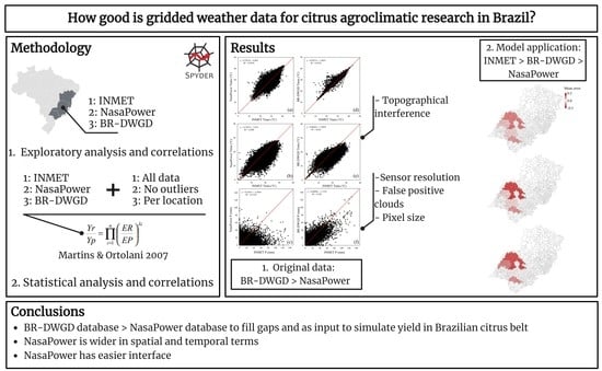
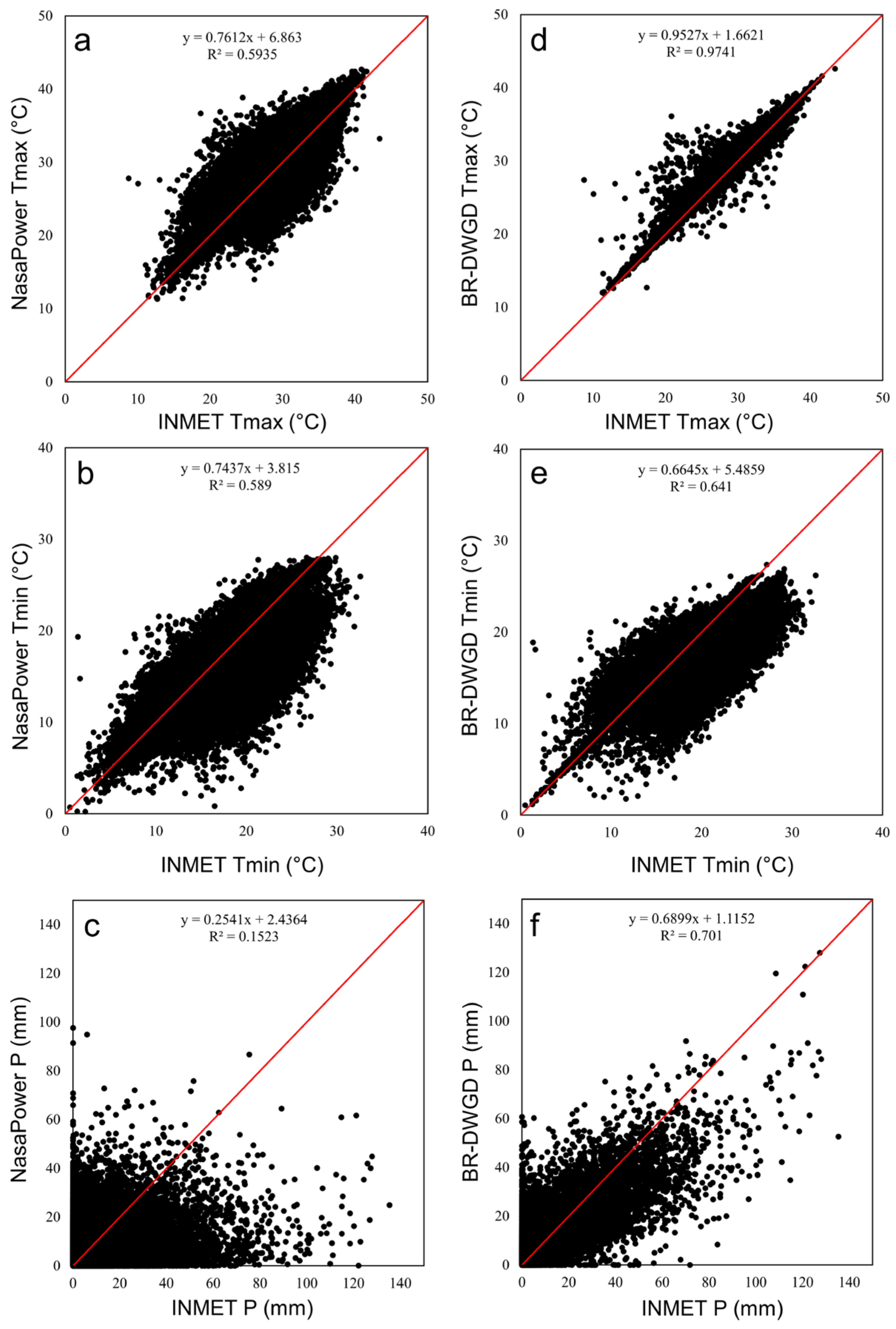
• RQ1: Do gridded data present a high correlation with in situ climatic data, allowing them to serve as a substitute or to fill potential gaps in measured data?
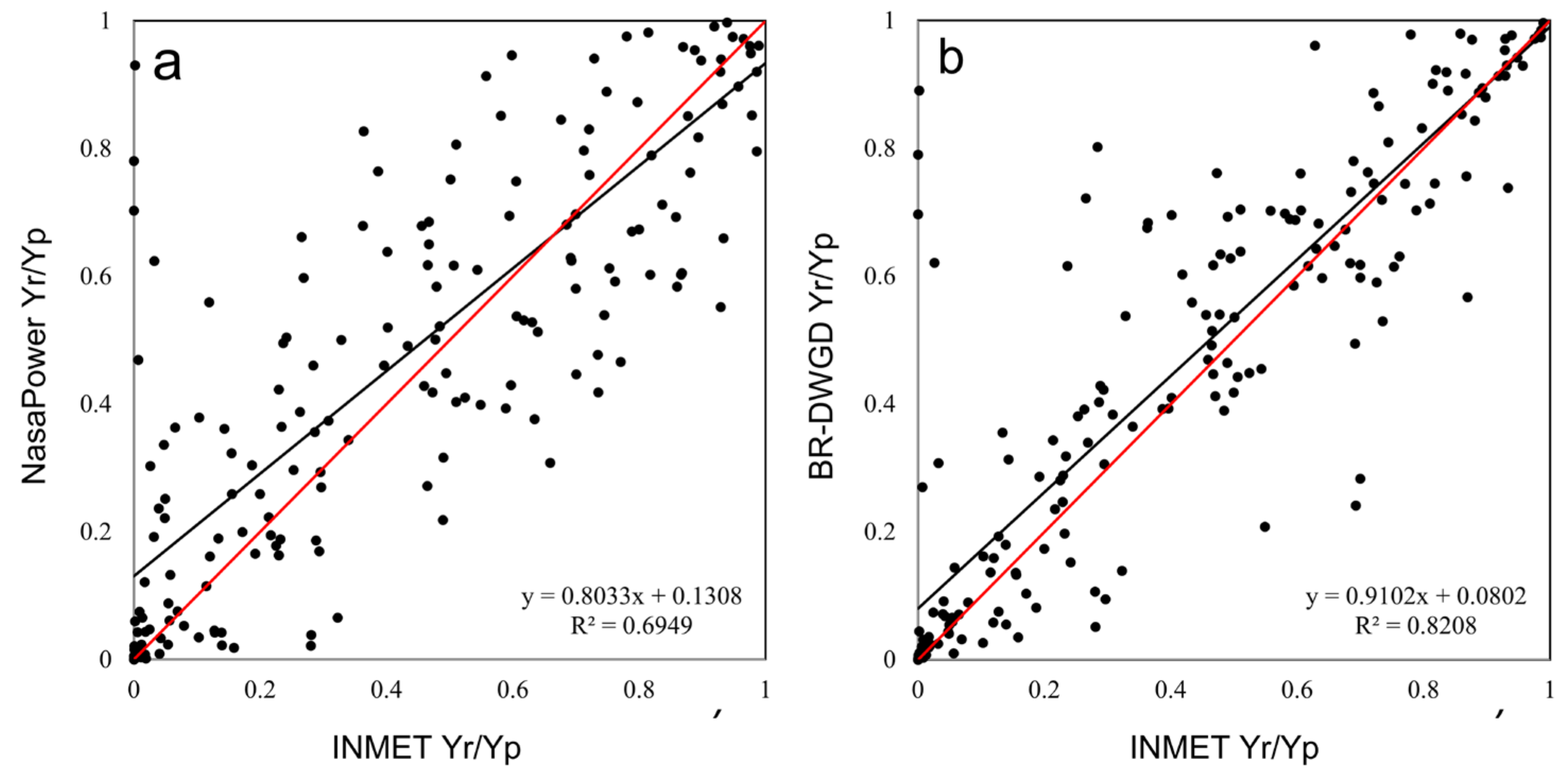
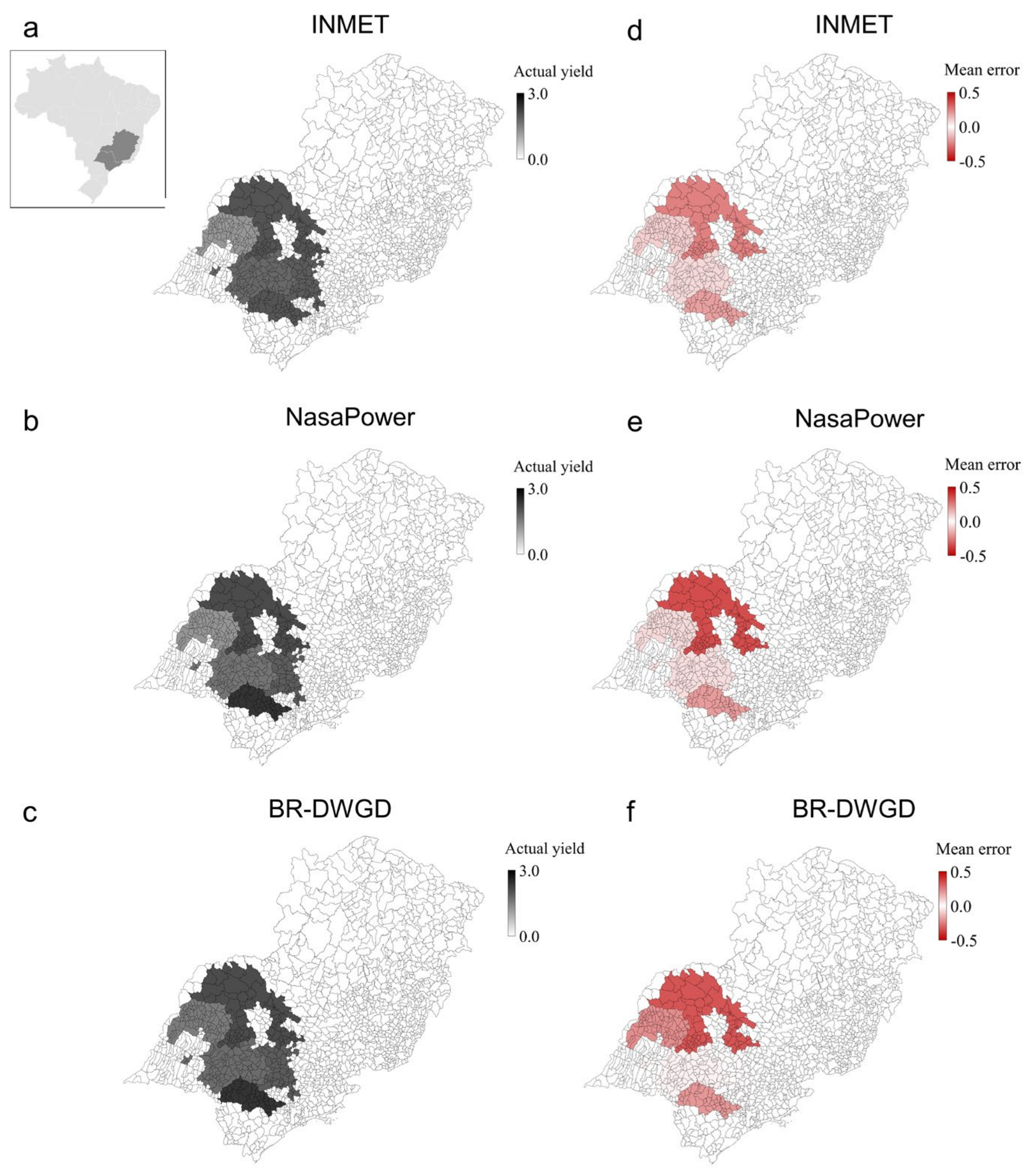
• RQ2: How do gridded data impact simulated sweet orange yield, using in situ data as a baseline for comparison?

The main objectives of this work are (i) to compare the main climatic data inputs options for predicting sweet orange yield in Brazil (which could also be used for other crops and areas); and (ii) to conduct a case study to evaluate the potential impacts of substituting in situ weather station data for gridded data (allowing better spatial and temporal coverage by filling gaps in the available in situ data). Both contributions may have a direct impact on improving the predictions in areas with lower weather station densities. Additionally, the same methodology could be applied to other crops, areas, and countries.

The work was organized into the following sections: Section 2. presents the materials and methods used in the case study; Section 3. describes and discusses the main results obtained in the case study; and Section 4. concludes the work, presenting the final remarks, limitations, and recommendations for future works.

1.1. Citrus Yield Prediction: Concepts and Models

A critical aspect of improving the decision-making processes of all links in the citrus supply chain is to predict the fruit volume produced in each season [19]. To account for different problems to estimate this volume, such as differences in planted areas between years, technologies, and processes used in different regions and the impact of extreme weather events, it is more beneficial to predict the yield instead of the total volume produced. A better yield prediction would allow the farmers to plan his/her processes better, the industries that produce inputs to better plan their production processes, the processing industries to estimate production and input sourcing, and the distribution agents to plan their logistics [20].

Predicting citrus yield is a challenging task. As perennial crops, they consist of several species and cultivars with different characteristics and resilience towards soil characteristics, pests, diseases, and the impact of extreme weather events, among other factors. Therefore, it is difficult to determine which variables should be used in a yield prediction model. Most studies used correlations of yield data with raw climatic data, mainly precipitation and temperature [21,22]. Additionally, it is crucial to observe that few works in the literature used correlations of processed data and model outputs, such as evapotranspiration and water deficit [20,23].

The use of processed data and climate indices (instead of the raw physical variables such as precipitation and temperature) should generate better prediction models because they capture more information from the original data [20,23]. For example, indices such as the Standardized Precipitation Index (SPI) and The Standardized Precipitation Evapotranspiration Index (SPEI) better capture the potential impact of droughts on crop yield than the use of only temperature and precipitation [24]. The work by Da Silva et al. [25] is an example of using an unsupervised machine learning model to predict sugarcane crop yield in different cities in São Paulo state, Brazil, using the SPI as one input of a prediction model.

One interesting aspect is that only some studies in the literature developed models with sequential equations that result in estimating yield. Several works, such as Ruß et al. [6] and Everingham et al. [8], used machine learning and artificial intelligence models, which are data-driven models that do not depend on sequential equations and extract information from the dataset. However, due to the data-driven nature of this approach, it does not incorporate important knowledge accumulated through decades of experimental studies and in situ crop yield research.

Agrometeorological models, on the other hand, tend to incorporate this knowledge in the equations that constitute the model [18,19,20,23,26]. This allows for better predictions in scenarios with a small volume of data but tends to finetune the model for a specific crop, variety, area, and weather pattern [27]. Nevertheless, using agrometeorological models based on sequential equations is the traditional approach for citrus yield prediction [18,19,20,23,26]. Therefore, this approach will be used in this work.

Despite similar objectives, five of the most important yield prediction models utilized in sweet oranges show different outputs, encompassing yield, fruit volume, fruit quality, and water productivity (

Table 1. Characteristics of five of the most important yield prediction models for sweet oranges.

Reference	Cultivar	Inputs	Data Source	Outputs
[28]	‘Natal’ sweet orange	Tmax, Tmin, CO2	In situ	WP (g/m2 mm)
[18]	‘Valencia’ sweet orange	Tmax, Tmin, P	In situ	Yield (fruits/box)
[29]	‘Valencia’ and ‘Navel’ sweet oranges	Tmax, Tmin, P, SR, W, RH	Gridded	NF and FS
[26]	‘Valencia’ sweet orange	Tmax, Tmin, P	In situ	Yield (fruits/box)
[19,21]	‘Valencia’ and ‘Navel’ sweet oranges	Tmax, Tmin, P, SR, W, RH	In situ	NF and FS

Legend: Tmax—maximum temperature; Tmin—minimum temperatures; P—precipitation; CO₂—gas carbonic air concentration; SR—solar radiation; W—wind velocity; RH—relative humidity; WP—water productivity; NF—number of fruits; FS—fruit size.

).

Camargo et al. [26] and Martins and Ortolani [18] adapted the Jensen [30] model for the ‘Valencia’ sweet orange. However, with the use of precipitation and temperature data to calculate potential (PET) and actual evapotranspiration (AET), the calculation method decided by the authors penalized the yield according to the water conditions in critical phenological stages of the crop.

The approach to correlate fruit yield and water deficit using AET and PET as central components of yield estimation is not new for crop yield prediction, especially in regions that experience droughts. An important agrometeorological model, the AEZ-FAO [31], adapted for maize, sugarcane, wheat, and other crops, has in its base equation the evapotranspiration (referred to as ET). Fadel [32] applied the AEZ-FAO model to predict the yield of seven mandarine cultivars, using different indices of sensitivity to water stress for each critical phenological stage.

Considering the water balance effect on yield and seeking to develop a simulation model for growth responses to climate change, Pereira et al. [28] studied the implications of atmospheric concentrations of CO₂ and variations in air temperature on water use efficiency. The authors developed the model using ‘Natal’ sweet orange and obtained a practical model to analyze several potential climate change scenarios. This is essential to improve the quality of decision-making throughout the supply chain and the resilience of citrus production.

Tubiello et al. [29] applied the yield estimation model of ‘Valencia’ sweet oranges developed by Ben Mechlia and Carroll [19] to predict the potential yield in relevant future climate scenarios for 2030 and 2090. This model estimates the number of fruits and final fruit size, as well as the growth of ‘Navel’ and ‘Valencia’ sweet oranges, using as inputs the orchard’s age, planting density, previous year yield, and meteorological variables such as temperature, precipitation, and cold and heat-related indices.

Most studies and model applications have used in situ sources of input data [18,19,20,26,27]. However, other important studies have used a gridded database as a source for input data [33,34,35,36].

Except for the Ben Mechlia and Carroll [19,37] model, all the cited works were elaborated based on data collected from cities and States located in Brazil, involving lower weather station densities than those in developed countries. Using datasets with a broader spatial coverage could result in models for yield prediction in lower-density areas, improving those countries’ decision-making regarding citrus supply chains.

1.2. In Situ and Gridded Data for Crop Yield Prediction

As observed throughout this work, high-quality input data is essential to provide accurate yield predictions. This is the case for both traditional agrometeorological models based on sequential equations and machine learning models based on complete data-driven methods. This also applies to hybrid models (also called physics-based machine learning models), which are starting to be explored in the literature.

Actual data obtained from correctly calibrated and well-maintained physical weather stations are always the best choice to provide high-quality inputs since they are real-time collected information [11]. Data from simulations and interpolations may contain several errors due to the assumptions used [38].

However, weather stations or in situ data can present gaps in the datasets and potential outliers that may be difficult to detect. Additionally, in many situations in developing countries, it is possible to observe both a lack of spatial coverage (due to the low density of weather stations in some areas) and of temporal coverage (due to station malfunction or stations that may have been only recently installed) [39].

Gridded databases provide an alternative for addressing the lack of spatial and temporal coverage. Additionally, this resource can be used to correct outliers and fill data gaps. Several works in the literature have explored using gridded datasets for crop yield prediction [28,40,41,42]. However, only a few studies, such as Bai et al. [38]; Bender and Sentelhas [43]; Battisti et al. [44] and Duarte and Sentelhas [11], aimed to compare in situ and gridded data, which is essential for helping the modeler or decision-maker to choose which data sources to use on his/her crop yield prediction model. In this work, we aimed to address this gap and to provide a methodology for other researchers and practitioners to compare and to choose databases for crop prediction models.

Bai et al. [38] and Duarte and Sentelhas [11] compared NasaPower data with weather station data to simulate maize yield in China and Brazil, respectively. Both authors identified problems in using only the NasaPower data in the model application, demanding other sources to complement NasaPower temperature and precipitation data. Monteiro et al. [12] also analyzed the NasaPower data as input in a sugarcane prediction model. The authors indicated the need for several adjustments, since this database did not provide satisfactory quality for wind speed, relative humidity, and precipitation estimation.

Other databases were also tested for yield modeling in substitution for real weather stations, such as AgMERRA (AgMIP Modern-Era Retrospective Analysis for Research and Applications) [44,45] and BR-DWGD [11,44]. AgMERRA and NasaPower were considered satisfactory in estimating soybean yield in Brazil [44].

2. Materials and Methods

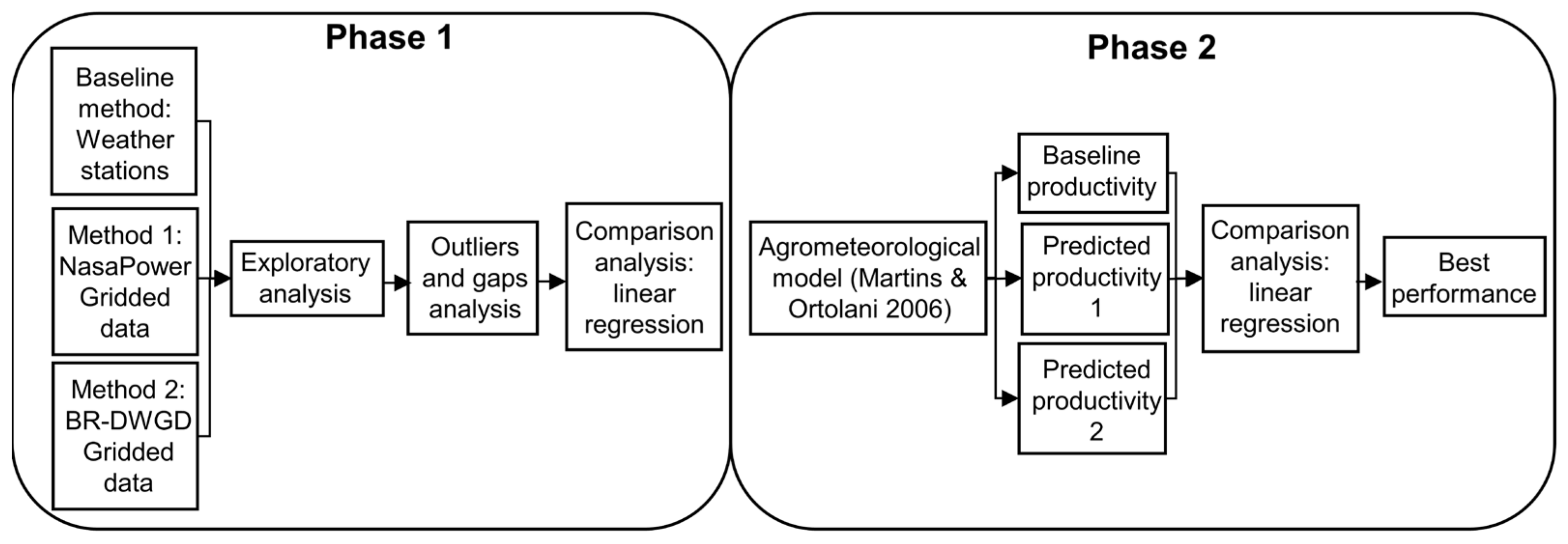
This work was elaborated in two phases (Figure 1). In Phase 1, called Scenario Evaluation, we generated and evaluated three relevant scenarios: (i) all data (without removing potential outliers); (ii) data without potential outliers; and (iii) all data, but separated into one dataset per state. Those scenarios encompass different traditional approaches for processing the inputs of the agrometeorological model and are essential for better extracting information from the data.

These scenarios also help to answer two critical questions: (i) What is the impact of removing potential outliers from the data? (ii) Should the analysis consider all data available, or should it separate the data considering spatial factors? Both are relevant for Brazil due to the significant differences between weather, soil, and agricultural processes in the different citrus-producing regions.

Phase 2 was called Input Evaluation. It consisted of evaluating and comparing three different options of inputs for the agrometeorological model: (i) in situ weather stations, which are traditionally used (and will be considered the baseline for comparison in this work); (ii) NasaPower gridded data; and (iii) BR-DWGD gridded data Using gridded data would allow better coverage of the production sites. It is essential to observe that Phase 2 also considered an in-depth exploratory data analysis and an analysis of outliers and gaps in the data for all considered scenarios and inputs.

2.1. Study Area

The location selection was based on two relevant parameters for citrus production: (i) volume produced (an indication of the importance of an area); and (ii) physical-related variables, mainly focusing on climate variables. We aimed to encompass Brazil’s most important citrus-producing regions while considering areas with different climate patterns. Therefore, for the citrus belt (São Paulo and Minas Gerais states), more than one location was selected within each of the five production regions (north, northwest, center, south, and southwest).

Then, the available years and the elevation above sea level were considered within these regions. When there was no weather station close to the location, another site was selected, which was recurrent for the Northeast of Brazil. This was essential because the baseline for comparison was using INMET weather station data.

We have collected data from São Paulo, Minas Gerais, Bahia, and Sergipe states from ten, five, four, and one locations, respectively (Figure 2,

Table 2. Characterization of the selected locations for the case study, grouped by state.

State	City/ID	Lat (°)	Long (°)	Alt (m)	Y (t/ha)	Tmax (°C)	Tmin (°C)	P (mm)
SP	Avaré/1	−23.1	−48.9	766	44.82	27.4	21.1	977.8
	Bauru/2	−22.4	−49.0	537	31.32	29.7	17.7	839.8
	Bebedouro/3	−20.9	−48.5	573	32.38	31.3	24.5	1362.6
	Franca/4	−20.6	−47.4	1040	32.38	28.3	18.5	1304.4
	Itapeva/5	−24.0	−48.9	717	44.82	26.8	16.3	1257.6
	Jales/6	−20.2	−50.6	478	25.69	31.7	18.8	694.0
	Piracicaba/7	−22.7	−47.6	554	33.28	29.1	16.8	1059.2
	Porto Ferreira/8	−21.9	−47.5	559	33.28	29.3	15.8	1078.2
	São Carlos/9	−22.0	−47.9	856	31.32	28.0	16.9	1408.2
	Votuporanga/10	−20.4	−50.0	525	25.69	32.5	18.9	1125.4
MG	Campina Verde/11	−19.5	−49.5	532	32.38	31.8	24.5	1284.8
	Planura/12	−20.2	−48.7	492	32.38	31.9	21.2	2522.1
	Sacramento/13	−19.9	−47.4	832	32.38	29.5	22.5	1299.4
	Uberaba/14	−19.7	−48.0	823	32.38	30.1	17.9	1661.6
	Uberlândia/15	−18.9	−48.3	863	32.38	29.9	19.4	1260.0
BA	Euclides da Cunha/16	−10.5	−39.0	472	13.07	31.8	20.9	446.0
	Feira de Santana/17	−12.2	−39.0	234	13.07	31.3	20.5	736.4
	Itiruçu/18	−13.5	−40.1	820	13.07	28.1	17.2	683.4
	Ribeira do Amparo/19	−11.1	−38.4	186	13.07	32.9	20.6	476.2
SE	Brejo Grande/20	−10.5	−36.5	30	13.97	31.6	26.4	1040.2

Source: INMET (INMET Weather stations available at: https://bdmep.inmet.gov.br/ accessed on 13 September 2022) dataset. Legend: SP—São Paulo; MG—Minas Gerais; BA—Bahia; SE—Sergipe; Lat—latitude; Long—longitude; Alt—altitude; Y—estimated production for the 2021/22 harvest by Fundecitrus (SP and MG) and IBGE (BA and SE); Tmax—maximum temperature average for 2019; Tmin—minimum temperature average for 2019; P—total precipitation for 2019.

). This data collection region distribution roughly reflects each state’s importance for citrus production. The time interval of data collection was from 1 January 2010 to 12 December 2020, resulting in 10 years of daily observations for climate data. Usable data from 20 stations were obtained, resulting in 73,521 observation points for each climate variable.

2.2. Data Collection

Daily data of maximum temperature (Tmax—°C), minimum temperature (Tmin—°C), and precipitation (P—mm) inputs for Phases 1 and 2 were obtained from the following three different sources: INMET, NasaPower (NasaPower data available at: https://power.larc.nasa.gov/data-access-viewer/ accessed on 13 September 2022), and BR-DWGD (BR-DWGD data available at: https://utexas.box.com/Xavier-etal-IJOC-DATA accessed on 14 September 2022). The observed data, used as a reference, were obtained from INMET weather stations for each location (Table 2).

The gridded data were obtained from two databases: NasaPower and BR-DWGD [17]. NasaPower data were downloaded via the Internet from the NasaPower website. The BR-DWGD data were downloaded using a Python script and archives (nc) prepared and provided by the authors using Python.

All data were inserted into a single dataframe for processing and knowledge extraction.

2.3. Data Processing and Scenario Generation

As previously described (Section 2.1.), three relevant scenarios were analyzed in the case study: (i) all available data (without removing potential outliers); (ii) data with outliers removed using the Boxplot method [46]; and (iii) data separated by states (without removing potential outliers).

In scenario (ii), the outliers of each city were identified using the interquartile (IQR) method, also known as the Boxplot method [46]. The IQR is the difference between the 75th and the 25th percentiles. For maximum and minimum temperatures, a multiple of 3× IQR was used. For precipitation, a multiple of 5× IQR was used, as 3× IQR still encompassed data that were not identified as outliers. All potential outliers were eliminated from the dataframe in this scenario. The Climpact R package was used to analyze the data, and outliers were eliminated using a Python script.

The agrometeorological model developed by Martins and Ortolani [18] was then applied to each scenario. Linear regressions were used to analyze the results and compare the models’ outputs using INMET climate data and gridded data (NasaPower and BR-DWGD). Our main objective was to explore the results of the agrometeorological model using two different gridded datasets as inputs compared to the INMET baseline as input.

The regressions were analyzed using the following statistical metrics: mean error (ME); mean absolute error (MAE); root mean square error (RMSE); agreement index (d) [47]; coefficient of determination (R²); and confidence index (C) [48]. The main Python libraries used in this step were Pandas (https://pandas.pydata.org/ accessed on 20 September 2022) and Numpy (https://numpy.org/ accessed on 20 September 2022).

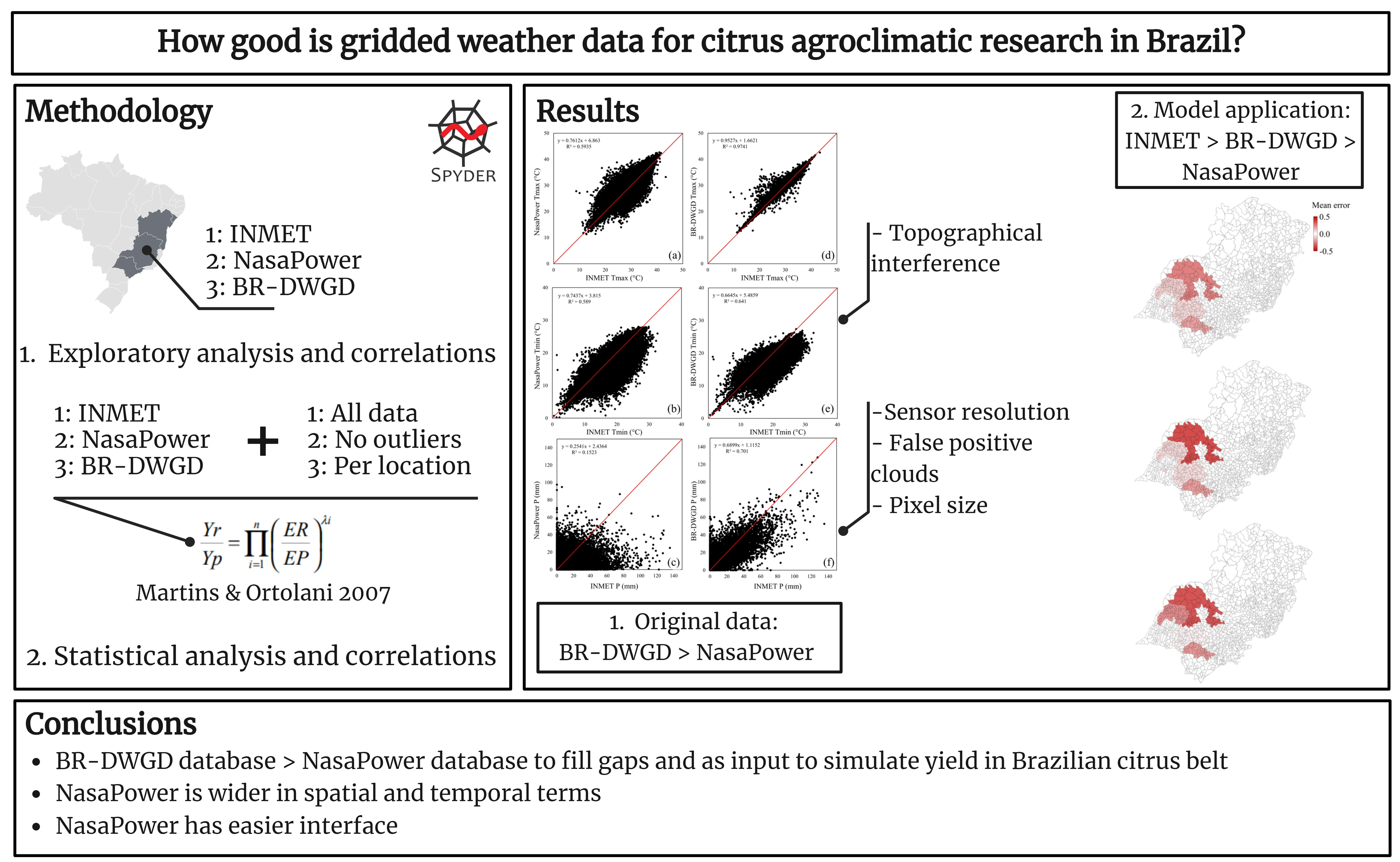
2.4. Data Quality Analysis

After determining the best data processing scenario, a data quality analysis was applied to the gridded data in Phase 2, following the methodology by [11]. For each climatic variable (Tmax, Tmin, and P) and Eto calculated, a linear regression analysis was conducted between observed data (INMET baseline) and gridded data. Besides daily analysis, the data were aggregated and analyzed monthly and annually in order to better identify trends in the data. All the results were analyzed using the metrics described above. The main Python libraries used in this step were Pandas and Matplotlib (https://matplotlib.org/ accessed on 20 September 2022).

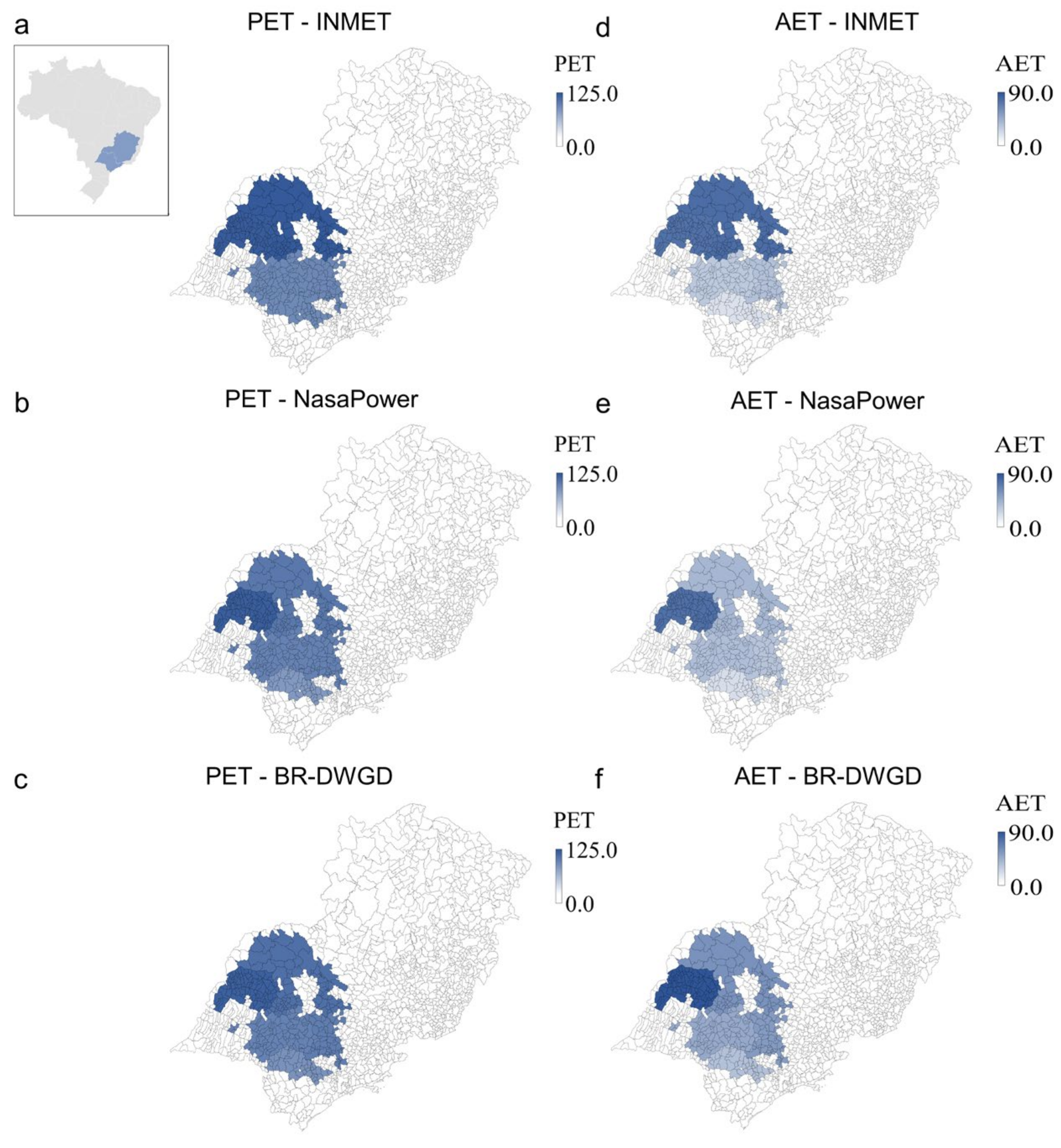
2.5. Agrometeorological Model Application

We used the agrometeorological model described by Martins and Ortolani [18] for ‘Valencia’ sweet orange (Citrus sinensis Osbeck) to simulate the relation between attainable yield and potential yield. As already mentioned, this is an important and thoroughly validated model to predict citrus yield in Brazil, notably in the Southwest region.

First, for each location and year, the potential (PET) and actual evapotranspiration (AET) were calculated by the Thorthwaite and Mather [49] method considering a soil moisture storage capacity of 100 mm, a standard used value [18,26]. The WaterbalANce app [50] was used to calculate PET and AET.

The agrometeorological model was then applied for each location, using the second combination of phenological phases tested by the authors, which showed the best performance [18]. All the results were analyzed using the error metrics described in Section 2.3.

Lastly, a spatial analysis of the results was conducted, generating and analyzing evapotranspiration and yield maps for each input data method only in the citrus belt region, considering the mean values of the locations selected within each region. Mean error maps were also elaborated, comparing model outputs with mean values for each citrus belt region for eight harvests from the sweet Orange Crop Forecast (Fundecitrus). Those maps allow a better spatial analysis of the models’ results, generating further insights to help decision-making.

3. Results

The results presented herein were based on scenario (i), in which all regions were considered together, and no potential outliers were removed. This is the most common scenario analyzed in the literature, as in the works by Battisti et al. [44] and Duarte and Sentelhas [11].

Except for Tmin, the BR-DWGD data showed the best performance compared with the INMET data in all time scales (

Table 3. Phase 2: Comparison between INMET and gridded weather data on daily, monthly, and annual time scales and their respective errors and performance indices.

Source	Variable	Scale	Mean (±s.d.)	C.V.	r	R2	d	C
NasaPower	P	Daily	3.3 (±6.2)	1.88	0.39	0.15	0.57	0.22
		Monthly	95.4 (±83.1)	0.87	0.85	0.72	0.91	0.78
		Annual	1047.7 (±384.6)	0.37	0.83	0.68	0.89	0.74
	Tmax	Daily	28.9 (±3.8)	0.13	0.77	0.59	0.88	0.67
		Monthly	28.9 (±3.1)	0.11	0.80	0.65	0.89	0.72
		Annual	29 (±1.9)	0.07	0.71	0.51	0.84	0.60
	Tmin	Daily	17.9 (±3.9)	0.21	0.77	0.59	0.86	0.66
		Monthly	17.9 (±3.5)	0.19	0.80	0.64	0.87	0.69
		Annual	18 (±2.4)	0.13	0.69	0.48	0.79	0.55
BR-DWGD	P	Daily	3.5 (±7.9)	2.24	0.84	0.70	0.90	0.76
		Monthly	101.8 (±95.8)	0.94	0.95	0.90	0.97	0.92
		Annual	1121.3 (±434.4)	0.39	0.94	0.88	0.97	0.91
	Tmax	Daily	29.3 (±3.7)	0.13	0.99	0.97	0.99	0.98
		Monthly	29.3 (±2.7)	0.09	0.99	0.97	0.99	0.98
		Annual	29.3 (±1.7)	0.06	0.98	0.96	0.98	0.96
	Tmin	Daily	18.1 (±3.3)	0.18	0.80	0.64	0.87	0.70
		Monthly	18.1 (±2.8)	0.15	0.77	0.60	0.85	0.66
		Annual	18.2 (±1.7)	0.09	0.61	0.37	0.61	0.44

Legend: s.d.—standard deviation; C.V.—coefficient of variation; d—agreement index; r—Pearson coefficient; R²—coefficient of determination; C—confidence index; P—precipitation; Tmax—maximum temperature; Tmin—minimum temperature.

and Figure 3). That means that the BR-DWGD data provides higher-quality results than the NasaPower data, considering the agrometeorological model and the specific regions. The higher precision of BR-DWGD data is due to a methodology that interpolates weather station data from INMET and the National Water Agency (Agência Nacional de Águas—ANA), which are more accurate than satellite data.

Specifically for the minimum air temperature, the BR-DWGD database reduced the r, d, and C indices. Six of the twenty cities studied here presented statistical indices lower than 0.5 for this variable. Xavier et al. [51] identified that Tmin and wind speed variables have the highest number of days with inhomogeneous data. The authors could not establish a single cause. Some potential causes were defective instruments and using different units [51]. Although they did not find a reason for this specific problem on Tmin, the stations from those six cities probably presented a homogeneity problem, influencing the BR-DWGD calculation method. This resulted in better results for the NasaPower database in the final dataset.

The differences between INMET and NasaPower databases are probably related to several factors, such as sensor resolutions, pixel size from the satellites, or even geographical differences between satellite records and weather station measurements [38]. A large dispersion was observed for P daily data (Figure 3c), especially when using NasaPower, resulting in the worst R² (0.15), d (0.57), and C (0.22).

On the other hand, the P daily data provided by the BR-DWGD database (Figure 3f) presented better performance and indices (R² = 0.70, d = 0.90, and C = 0.76). This agrees with several previous research articles, such as Monteiro et al. [12] and Van Wart et al. [13], who observed that p values estimated by NasaPower always showed the worst correlation with measured data. These results occur due to the difficulty of estimating light and extreme precipitations and avoiding false positives for precipitation clouds in simulation methods [52].

Our findings agree with other works which evaluated the quality of weather data for different modeling applications [11,12,38,43,44,53]. A possible explanation for the errors is the topographic influence in temperature estimation, as White et al. [53] observed in mountainous regions.

The aggregation of P data on monthly and annual scales increased the correlation indices for both gridded databases due to the reduction of data dispersion (Table 3). It is important to emphasize that the primary variable considered by the model is AET, which is highly affected by soil water balance and precipitation. The PET and AET calculated in the model by Martins and Ortolani [18] applied the Thorthwaite and Mather [49] methods, which use monthly data as an input.

The PET and AET estimated by the BR-DWGD database (r = 0.92) presented better results than the NasaPower database (r = 0.85) compared to INMET evapotranspiration values (Figure 4). Additionally, those values were significantly lower than the original daily data.

The variations between PET (125 mm maximum) and AET (90 mm maximum) are the main factors responsible for the relations between attainable yield (Yr) and potential yield (Yp) (Figure 4). It is possible to observe an underestimation of PET and AET when using a gridded database compared to the baseline in all citrus belt regions (Figure 4). This is probably due to those databases’ temperature and precipitation estimation errors [44]. Therefore, as expected, it is essential to use high-quality data since it will directly affect PET and AET determination.

In the present study, the BR-DWGD database presented better results regarding precipitation and, consequently, AET, which was observed in other applications [44]. An alternative to using the NasaPower database is using other sources such as the ANA database to substitute the precipitation data [12]. Duarte and Sentelhas [11] obtained better results for maize yield simulation using NasaPower and ANA precipitation data rather than only NasaPower data. This could be a strategy to improve the quality of the results observed in this work.

In order to answer our first question, i.e., if gridded data were good enough for filling gaps or substituting measured data, the BR-DWGD database presented significant correlation indices with the INMET baseline. It could be used to fill data gaps or even for locations with little data in Brazil since the database is limited to this country. However, this gridded database includes only data from 1961 to 2020, making it necessary to use NasaPower for more recent years. Additionally, the NasaPower interface is easier to use for non-programmers since the BR-DWGD database requires more advanced knowledge in this field.

Table 4. Phase 1: Comparison between Yr output from Martins and Ortolani [18] model using INMET and gridded database and their respective errors and performance indices, considering three scenarios.

Source	Scenario	Index
		RMSE	ME	ME (kg/Plant)	MAE	MAE (kg/Plant)	d	r	R2	C
NasaPower	(i) All data	0.21	0.03	9.86	0.15	43.77	0.91	0.83	0.69	0.76
	(ii) Outliers removed	0.12	0.07	21.15	0.07	21.53	0.39	0.49	0.24	0.19
	(iii) Separated by states—SP	0.22	−0.01	−4.14	0.14	42.45	0.8	0.64	0.4	0.51
	(iii) Separated by states—BA + SE	0.21	0.04	11.46	0.14	41.55	0.6	0.37	0.14	0.22
	(iii) Separated by states—MG	0.3	0.15	43.27	0.24	71.7	0.77	0.66	0.43	0.51
BR-DWGD	(i) All data	0.17	0.04	10.6	0.1	28.67	0.95	0.91	0.82	0.86
	(ii) Outliers removed	0.03	0.01	2.61	0.01	3.96	0.9	0.84	0.71	0.76
	(iii) Separated by states—SP	0.16	0.05	15.44	0.09	27.43	0.89	0.81	0.66	0.73
	(iii) Separated by states—BA + SE	0.15	−0.04	−11.41	0.09	27.49	0.66	0.54	0.29	0.36
	(iii) Separated by states—MG	0.21	0.09	27.15	0.15	44.07	0.88	0.83	0.69	0.73

Legend: the scenario with the best performance for data quality analysis is highlighted. SP—São Paulo; MG—Minas Gerais; BA—Bahia; RMSE—root mean square error; ME—mean error; MAE—mean absolute error; d—agreement index; r—Pearson coefficient; R²—coefficient of determination; C—confidence index.

illustrates the comparison results using the NasaPower, BR-DWGD, and INMET data as inputs for the Martins and Ortolani [18] agrometeorological model. It contains the error metrics and correlation results for the four scenarios. Due to the high dispersion observed in p values when using the NasaPower database and the better temperature data correlations with INMET, the BR-DWGD database resulted in a better yield estimation using the agrometeorological model.

Regarding the relation between attainable yield (Yr) and potential yield (Yp) outputs considering the NasaPower and BR-DWGD inputs, besides the input sources, the methodology for processing the input data is also relevant (Figure 5). Herein, the best scenario for data quality analysis was using all locations together and not removing the outliers identified in the analysis (Table 4).

When removing the outliers (scenario (ii)), the errors were reduced, especially RMSE, which is closely related to outliers. However, as the main outliers identified were from P data as extreme values, removing them resulted in underestimating attainable yield (Yr), reducing the Yr/Yp relation. It is vital to observe that estimating extreme values is a problem in satellite precipitation estimation by algorithms [54]. Different remotely sensed products for P estimation show substantial differences in representing P extremes [54,55]. Overall, there is always a tendency to miss a significant P volume when using those algorithms [54].

When applying the agrometeorological model separately for each State (scenario (iii)), there was a reduction in the quality of results (R² < 0.45 and C < 0.51 for NasaPower and R² < 0.7 and C < 0.75 for BR-DWGD), using gridded data, comparing to applying the model for all States simultaneously (R² = 0.69 and C = 0.76 for NasaPower and R² = 0.82 and C = 0.86 for BR-DWGD). The worst results were for Bahia State, probably due to the low density of stations, leading to a smaller quantity of data and reducing the quality of data interpolations.

Figure 6 illustrates the maps of the attainable and potential yields and the mean errors for the agrometeorological model using the different inputs analyzed in this work. First, there was a tendency to overestimate the yield when using the agrometeorological model, inherent to the model itself, as identified by its authors [18]. Our results indicate that this is even more pronounced when using the gridded databases. In Figure 6e,f, it is possible to observe that the peripherical regions of the citrus belt (north and southwest) presented higher errors. This was mainly due to the PET underestimation, which reduced the Yr/Yp relation and increased the errors.

Therefore, to answer our second question, i.e., if gridded data presented similar quality to measured data in simulating yield, the answer is yes. The BR-DWGD database presented significant correlation indices with the INMET baseline. Nevertheless, in specific scenarios, the NasaPower database can also be used as an input source when analyzing recent years or locations outside Brazil.

Using agrometeorological models is essential for agricultural decision-making, and high-quality input data are crucial for satisfactory results [38]. As already discussed, there are different types of climatic databases, each with advantages and flaws [56]. An alternative to obtaining accurate outputs is to use the best sources, which makes data quality analysis an essential step in this process. The methodology used in this work could be adapted for use on other crops, areas, and periods.

4. Conclusions

High-quality data are essential for agricultural decision-making. One crucial aspect that depends directly on data and processing quality is yield prediction, which is essential for decision-making in citrus supply chains. However, many areas lack climate data, which are primary inputs of the different agrometeorological models.

In this work, we analyzed the potential use of the two gridded databases to fill gaps in historical climate variables series, considering both areas with higher and lower weather station density. An agrometeorological model was used to predict the yield of ‘Valencia’ sweet orange in different regions in Brazil.

Our results suggest that the BR-DWGD database is better than the NasaPower database at filling gaps and being used as an input to simulate attainable yield in the Brazilian citrus belt. However, due to the geographical and temporal limitations of the BR-DWGD database, NasaPower is still an alternative in some specific cases. Additionally, when using NasaPower, it is recommended to use a measured precipitation source (such as INMET, ANA, or a weather station available on site) for obtaining outcomes with the lowest errors and highest precision and accuracy since the main limitation of this database is poor precipitation simulation.

Despite the low quality of precipitation data from NasaPower, this database is more accessible and easier to use than BR-DWGD. Combining its data with data from other databases may provide better insights for decision-making. Lastly, a data quality analysis, such as the one presented in this work, must be conducted for every yield prediction task.

Alongside the conclusions described above, this study testifies the data quality of gridded databases for citrus yield research in the Brazilian citrus belt region, the second biggest producer of citrus and the biggest producer of sweet orange of the world. We also analyze the recent actualization of the BR-DWGD database for agroclimatic research.

The limitations of this study were as follows: (i) only one agrometeorological model was used; (ii) no machine learning yield prediction model was used; and (iii) the model used was based on yield penalization by water deficit, which is very relevant for the Brazilian context. Future works must focus on the following: (i) evaluating more gridded databases; (ii) conducting case studies for other crops, varieties, regions, and countries; (iii) evaluating the use of other agrometeorological and machine learning models; and (iv) evaluating other important model inputs, such as solar radiation. Additionally, it would be interesting to explore the quality of the results when combining multiple gridded databases or using model ensembles.

References

1. IPCC. IPCC Summary for Policymakers. In Climate Change 2022: Impacts, Adaptation and Vulnerability. Contribution of Working Group II to the Sixth Assessment Report of the Intergovernmental Panel on Climate Change; Pörtner, H.-O., Roberts, D.C., Tignor, M., Poloczanska, E.S., Mintenbeck, K., Alegría, A., Craig, M., Langsdorf, S., Löschke, S., Möller, V., Okem, A., Rama, B., Eds.; Cambridge University Press: Cambridge, UK; New York, NY, USA, 2022; pp. 3–33. [Google Scholar]
2. Sukumar Chakraborty, S.C.; Luck, J.; Hollaway, G.; Freeman, A.; Norton, R.; Garrett, K.A.; Percy, K.; Hopkins, A.; Davis, C.; Karnosky, D.F. Impacts of Global Change on Diseases of Agricultural Crops and Forest Trees. CABI Rev. 2008, 2008, 1–15. [Google Scholar] [CrossRef]
3. Pollock, C.J. The Response of Plants to Temperature Change. J. Agric. Sci. 1990, 115, 1–5. [Google Scholar] [CrossRef]
4. De Ollas, C.; Morillón, R.; Fotopoulos, V.; Puértolas, J.; Ollitrault, P.; Gómez-Cadenas, A.; Arbona, V. Facing Climate Change: Biotechnology of Iconic Mediterranean Woody Crops. Front. Plant Sci. 2019, 10, 427. [Google Scholar] [CrossRef] [PubMed]
5. Vu, J.C.V. Photosynthesis, Growth, and Yield of Citrus at Elevated Atmospheric CO2. J. Crop Improv. 2005, 13, 361–376. [Google Scholar] [CrossRef]
6. Morgenthaler, S. Exploratory Data Analysis. WIREs Comp. Stat. 2009, 1, 33–44. [Google Scholar] [CrossRef]
7. Emmert-Streib, F.; Yang, Z.; Feng, H.; Tripathi, S.; Dehmer, M. An Introductory Review of Deep Learning for Prediction Models with Big Data. Front. Artif. Intell. 2020, 3, 4. [Google Scholar] [CrossRef]
8. Everingham, Y.L.; Smyth, C.W.; Inman-Bamber, N.G. Ensemble Data Mining Approaches to Forecast Regional Sugarcane Crop Production. Agric. For. Meteorol. 2009, 149, 689–696. [Google Scholar] [CrossRef]
9. Khaki, S.; Wang, L. Crop Yield Prediction Using Deep Neural Networks. Front. Plant Sci. 2019, 10, 621. [Google Scholar] [CrossRef]
10. Ruß, G.; Kruse, R.; Schneider, M.; Wagner, P. Data Mining with Neural Networks for Wheat Yield Prediction. In Advances in Data Mining. Medical Applications, E-Commerce, Marketing, and Theoretical Aspects; Perner, P., Ed.; Lecture Notes in Computer Science; Springer: Berlin/Heidelberg, Germany, 2008; Volume 5077, pp. 47–56. ISBN 978-3-540-70717-2. [Google Scholar]
11. Duarte, Y.C.N.; Sentelhas, P.C. NASA/POWER and DailyGridded Weather Datasets—How Good They Are for Estimating Maize Yields in Brazil? Int. J. Biometeorol. 2020, 64, 319–329. [Google Scholar] [CrossRef]
12. Monteiro, L.A.; Sentelhas, P.C.; Pedra, G.U. Assessment of NASA/POWER Satellite-Based Weather System for Brazilian Conditions and Its Impact on Sugarcane Yield Simulation: Sugarcane yield simulation with nasa/power satellite-based data. Int. J. Clim. 2018, 38, 1571–1581. [Google Scholar] [CrossRef]
13. Van Wart, J.; Grassini, P.; Yang, H.; Claessens, L.; Jarvis, A.; Cassman, K.G. Creating Long-Term Weather Data from Thin Air for Crop Simulation Modeling. Agric. For. Meteorol. 2015, 209–210, 49–58. [Google Scholar] [CrossRef]
14. Wart, J.; Grassini, P.; Cassman, K.G. Impact of Derived Global Weather Data on Simulated Crop Yields. Glob. Change Biol. 2013, 19, 3822–3834. [Google Scholar] [CrossRef]
15. Shepard, D. A Two-Dimensional Interpolation Function for Irregularly-Spaced Data. In Proceedings of the 1968 23rd ACM National Conference, 23–25 January 1968; pp. 517–524. [Google Scholar]
16. King, A.D.; Alexander, L.V.; Donat, M.G. The Efficacy of Using Gridded Data to Examine Extreme Rainfall Characteristics: A Case Study for Australia: Gridded rainfall extremes in Australia. Int. J. Climatol. 2013, 33, 2376–2387. [Google Scholar] [CrossRef]
17. Xavier, A.C.; Scanlon, B.R.; King, C.W.; Alves, A.I. New Improved Brazilian Daily Weather Gridded Data (1961–2020). Intl J. Climatol. 2022, 42, 8390–8404. [Google Scholar] [CrossRef]
18. Martins, A.N.; Ortolani, A.A. Estimativa de Produção de Laranja Valência Pela Adaptação de Um Modelo Agrometeorológico. Bragantia 2006, 65, 355–361. [Google Scholar] [CrossRef]
19. Ben Mechlia, N.; Carroll, J.J. Agroclimatic Modeling for the Simulation of Phenology, Yield and Quality of Crop Production. II. Citrus Model Implementation and Verification. Int. J. Biometeorol. 1989, 33, 52–65. [Google Scholar] [CrossRef]
20. Moreto, V.B.; de Rolim, G.S.; Zacarin, B.G.; Vanin, A.P.; de Souza, L.M.; Latado, R.R. Agrometeorological Models for Forecasting the Qualitative Attributes of “Valência” Oranges. Theor. Appl. Climatol. 2017, 130, 847–864. [Google Scholar] [CrossRef]
21. Tubelis, A.; Salibe, A.A.; Pessim, G. Relações Entre a Produção de Laranjeira ‘Westin’ e as Precipitações Em Botucatu, SP. Pesqui. Agropecuária Bras. 1999, 34, 771–779. [Google Scholar] [CrossRef]
22. Tubelis, A.; Salibe, A.A. Relações Entre a Produção de Laranjeira ‘Hamlin’ Sobre Porta-Enxerto de Laranjeira ‘Caipira’ e as Precipitações Mensais No Altiplano de Botucatu, SP. Pesqui. Agropecuária Bras. 1988, 23, 239–246. [Google Scholar]
23. Paulino, S.E.P.; Mourão Filho, F.d.A.A.; de Holanda Nunes Maia, A.; Avilés, T.E.C.; Dourado Neto, D. Agrometeorological Models for “Valencia” and “Hamlin” Sweet Oranges to Estimate the Number of Fruits per Plant. Sci. Agric. (Piracicaba Braz.) 2007, 64, 1–11. [Google Scholar] [CrossRef]
24. Vicente-Serrano, S.M.; Beguería, S.; López-Moreno, J.I. A Multiscalar Drought Index Sensitive to Global Warming: The Standardized Precipitation Evapotranspiration Index. J. Clim. 2010, 23, 1696–1718. [Google Scholar] [CrossRef]
25. Da Silva, R.F.; Gesualdo, G.C.; Benso, M.R.; Fava, M.C.; Mendiondo, E.M.; Saraiva, A.M.; Botazzo Delbem, A.C. A Data-Driven Framework for Identifying Productivity Zones and the Impact of Agricultural Droughts in Sugarcane Using SPI and Unsupervised Learning. In Proceedings of the 2021 IEEE International Workshop on Metrology for Agriculture and Forestry (MetroAgriFor), Trento-Bolzano, Italy, 3 November 2021; pp. 226–231. [Google Scholar]
26. Camargo, M.B.P.D.; Ortolani, A.A.; Pedro Júnior, M.J.; Rosa, S.M. Modelo Agrometeorológico de Estimativa de Produtividade Para o Cultivar de Laranja Valência. Bragantia 1999, 58, 171–178. [Google Scholar] [CrossRef]
27. Dourado-Neto, D.; Teruel, D.A.; Reichardt, K.; Nielsen, D.R.; Frizzone, J.A.; Bacchi, O.O.S. Principles of Crop Modeling and Simulation: I. Uses of Mathematical Models in Agricultural Science. Sci. Agric. 1998, 55, 46–50. [Google Scholar] [CrossRef]
28. Pereira, F.F.S.; Sánchez-Román, R.M.; Orellana González, A.M.G. Simulation Model of the Growth of Sweet Orange (Citrus sinensis L. Osbeck) Cv. Natal in Response to Climate Change. Clim. Change 2017, 143, 101–113. [Google Scholar] [CrossRef]
29. Tubiello, F.; Rosenzweig, C.; Goldberg, R.; Jagtap, S.; Jones, J. Effects of Climate Change on US Crop Production: Simulation Results Using Two Different GCM Scenarios. Part I: Wheat, Potato, Maize, and Citrus. Clim. Res. 2002, 20, 259–270. [Google Scholar] [CrossRef]
30. Jensen, M.E. Water Consumption by Agricultural Plants; Chapter 1; Academic Press: Cambridge, MA, USA, 1968. [Google Scholar]
31. Doorenbos, J.; Kassam, A.H. Yield Response to Water; Food and Agriculture Organization of the United Nations: Rome, Italy, 1979; p. 179. [Google Scholar]
32. Fadel, R.E.S. Influência Das Condições Agrometeorológicas Na Fenologia, Qualidade e Produtividade de Tangerinas Na Região de Capão Bonito. Ph.D. Thesis, Instituto Agronômico, Campinas, Brazil, 2011. [Google Scholar]
33. Fader, M.; von Bloh, W.; Shi, S.; Bondeau, A.; Cramer, W. Modelling Mediterranean Agro-Ecosystems by Including Agricultural Trees in the LPJmL Model. Geosci. Model Dev. 2015, 8, 3545–3561. [Google Scholar] [CrossRef]
34. Fares, A.; Bayabil, H.K.; Zekri, M.; Mattos-Jr, D.; Awal, R. Potential Climate Change Impacts on Citrus Water Requirement across Major Producing Areas in the World. J. Water Clim. Change 2017, 8, 576–592. [Google Scholar] [CrossRef]
35. Sugiura, T.; Sakamoto, D.; Koshita, Y.; Sugiura, H.; Asakura, T. Changes in Locations Suitable for Satsuma Mandarin and Tankan Cultivation Due to Global Warming in Japan. Acta Hortic. 2016, 91–94. [Google Scholar] [CrossRef]
36. Zabihi, H.; Ahmad, A.; Vogeler, I.; Said, M.N.; Golmohammadi, M.; Golein, B.; Nilashi, M. Land Suitability Procedure for Sustainable Citrus Planning Using the Application of the Analytical Network Process Approach and GIS. Comput. Electron. Agric. 2015, 117, 114–126. [Google Scholar] [CrossRef]
37. Ben Mechlia, N.; Carroll, J.J. Agroclimatic Modeling for the Simulation of Phenology, Yield and Quality of Crop Production. I. Citrus Response Formulation. Int. J. Biometeorol. 1989, 33, 36–51. [Google Scholar] [CrossRef]
38. Bai, J.; Chen, X.; Dobermann, A.; Yang, H.; Cassman, K.G.; Zhang, F. Evaluation of NASA Satellite- and Model-Derived Weather Data for Simulation of Maize Yield Potential in China. Agron. J. 2010, 102, 9–16. [Google Scholar] [CrossRef]
39. Rivington, M.; Bellocchi, G.; Matthews, K.B.; Buchan, K. Evaluation of Three Model Estimations of Solar Radiation at 24 UK Stations. Agric. For. Meteorol. 2005, 132, 228–243. [Google Scholar] [CrossRef]
40. Ali, M.F.; Abdul Aziz, A.; Williams, A. Assessing Yield and Yield Stability of Hevea Clones in the Southern and Central Regions of Malaysia. Agronomy 2020, 10, 643. [Google Scholar] [CrossRef]
41. Barbosa dos Santos, V.; Moreno Ferreira dos Santos, A.; da Silva Cabral de Moraes, J.R.; de Oliveira Vieira, I.C.; de Souza Rolim, G. Machine Learning Algorithms for Soybean Yield Forecasting in the Brazilian Cerrado. J. Sci. Food Agric. 2022, 102, 3665–3672. [Google Scholar] [CrossRef]
42. Torsoni, G.B.; de Oliveira Aparecido, L.E.; dos Santos, G.M.; Chiquitto, A.G.; da Silva Cabral Moraes, J.R.; de Souza Rolim, G. Soybean Yield Prediction by Machine Learning and Climate. Theor. Appl. Clim. 2023, 151, 1709–1725. [Google Scholar] [CrossRef]
43. Bender, F.D.; Sentelhas, P.C. Solar Radiation Models and Gridded Databases to Fill Gaps in Weather Series and to Project Climate Change in Brazil. Adv. Meteorol. 2018, 2018, 1–15. [Google Scholar] [CrossRef]
44. Battisti, R.; Bender, F.D.; Sentelhas, P.C. Assessment of Different Gridded Weather Data for Soybean Yield Simulations in Brazil. Appl Clim. 2019, 135, 237–247. [Google Scholar] [CrossRef]
45. Ruane, A.C.; Goldberg, R.; Chryssanthacopoulos, J. Climate Forcing Datasets for Agricultural Modeling: Merged Products for Gap-Filling and Historical Climate Series Estimation. Agric. For. Meteorol. 2015, 200, 233–248. [Google Scholar] [CrossRef]
46. Yang, J.; Rahardja, S.; Fränti, P. Outlier Detection: How to Threshold Outlier Scores? In Proceedings of the International Conference on Artificial Intelligence, Information Processing and Cloud Computing, Sanya, China, 19–21 December 2019; pp. 1–6. [Google Scholar]
47. Willmott, C.J. On the validation of models. Phys. Geogr. 1981, 2, 184–194. [Google Scholar] [CrossRef]
48. Camargo, A.P.; Sentelhas, P.C. Avaliação Do Desempenho de Diferentes Métodos de Estimativa da Evapotranspiração Potencial No Estado de São Paulo, Brasil. Rev. Bras. Agrometeorol. 1997, 5, 89–97. [Google Scholar]
49. Thornthwaite, C.W.; Mather, J.R. The Water Balance. Open J. Ecol. 2012, 2, 3. [Google Scholar]
50. Mammoliti, E.; Fronzi, D.; Mancini, A.; Valigi, D.; Tazioli, A. WaterbalANce, a WebApp for Thornthwaite–Mather Water Balance Computation: Comparison of Applications in Two European Watersheds. Hydrology 2021, 8, 34. [Google Scholar] [CrossRef]
51. Xavier, A.C.; King, C.W.; Scanlon, B.R. Daily Gridded Meteorological Variables in Brazil (1980–2013): Daily gridded meteorological variables in Brazil (1980–2013). Int. J. Climatol. 2016, 36, 2644–2659. [Google Scholar] [CrossRef]
52. Contractor, S.; Alexander, L.V.; Donat, M.G.; Herold, N. How Well Do Gridded Datasets of Observed Daily Precipitation Compare over Australia? Adv. Meteorol. 2015, 2015, 1–15. [Google Scholar] [CrossRef]
53. White, J.W.; Hoogenboom, G.; Stackhouse, P.W.; Hoell, J.M. Evaluation of NASA Satellite- and Assimilation Model-Derived Long-Term Daily Temperature Data over the Continental US. Agric. For. Meteorol. 2008, 148, 1574–1584. [Google Scholar] [CrossRef]
54. AghaKouchak, A.; Behrangi, A.; Sorooshian, S.; Hsu, K.; Amitai, E. Evaluation of Satellite-Retrieved Extreme Precipitation Rates across the Central United States. J. Geophys. Res. 2011, 116, D02115. [Google Scholar] [CrossRef]
55. Sylla, M.B.; Giorgi, F.; Coppola, E.; Mariotti, L. Uncertainties in Daily Rainfall over Africa: Assessment of Gridded Observation Products and Evaluation of a Regional Climate Model Simulation: Uncertainties in observed and simulated daily rainfall over africa. Int. J. Climatol. 2013, 33, 1805–1817. [Google Scholar] [CrossRef]
56. Aggarwal, P.K. Uncertainties in Crop, Soil and Weather Inputs Used in Growth Models: Implications for Simulated Outputs and Their Applications. Agric. Syst. 1995, 48, 361–384. [Google Scholar] [CrossRef]
Figure 1. Main components of this research [18].
Agriengineering 05 00057 g001
Figure 2. Map with the locations selected for the study. Legend: each number represents the city’s ID, also present in Table 2.
Agriengineering 05 00057 g002
Figure 3. Phase 2 results: Comparison of daily maximum temperature (a,d), minimum temperature (b,e), and precipitation (c,f) data from the NasaPower database (ac) and BR-DWGD database (df) versus INMET for ten-years from twenty Brazilian locations. Legend: each black circle represents a daily data point. The equation and determination coefficient of each variable is presented inside each chart.
Agriengineering 05 00057 g003
Figure 4. Potential evapotranspiration (PET) (mm) (ac); and actual evapotranspiration (AET) (mm) (df) maps of citrus belt regions output using INMET (a,d), the NasaPower database (b,e), and the BR-DWGD database (c,f). Legend: darker colors indicate higher values.
Agriengineering 05 00057 g004
Figure 5. Phase 2 results: Comparison of the relation between Yr and Yp output from Martins and Ortolani [18] model using the NasaPower database and INMET (a), and the BR-DWGD database and INMET (b) for twenty Brazilian locations. Legend: each black circle represents a Yr/Yp year value for one location. The black line indicates the correlation between the outputs, with the respective equation.
Agriengineering 05 00057 g005
Figure 6. Phase 2 results: Attainable yield (boxes per plant) maps of citrus belt regions output from Martins and Ortolani [18] model using INMET (a), the NasaPower database (b), and the BR −DWGD database (c). Mean error of estimated attainable yield maps of citrus belt regions when using Martins and Ortolani (2007) model with different climate input in relation to Orange Crop Forecast from Fundecitrus: INMET (d), NasaPower database (e), and BR −DWGD database (f).
Agriengineering 05 00057 g006