Article

A Comparative Analysis of Multi-Label Deep Learning Classifiers for Real-Time Vehicle Detection to Support Intelligent Transportation Systems

by
Danesh Shokri
1,2,*,
Christian Larouche
1,2 and
Saeid Homayouni
3
1
Département des Sciences Géomatiques, Université Laval, Québec, QC G1V 0A6, Canada
2
Centre de Recherche en Données et Intelligence Géospatiales (CRDIG), Université Laval, Québec, QC G1V 0A6, Canada
3
Centre Eau Terre Environnement, Institut National de la Recherche Scientifique, Québec, QC G1V 0A6, Canada
*
Author to whom correspondence should be addressed.
Smart Cities 2023, 6(5), 2982-3004; https://doi.org/10.3390/smartcities6050134
Submission received: 13 September 2023 / Revised: 17 October 2023 / Accepted: 18 October 2023 / Published: 23 October 2023
(This article belongs to the Special Issue Multidisciplinary Research on Smart Cities)

Abstract

:
An Intelligent Transportation System (ITS) is a vital component of smart cities due to the growing number of vehicles year after year. In the last decade, vehicle detection, as a primary component of ITS, has attracted scientific attention because by knowing vehicle information (i.e., type, size, numbers, location speed, etc.), the ITS parameters can be acquired. This has led to developing and deploying numerous deep learning algorithms for vehicle detection. Single Shot Detector (SSD), Region Convolutional Neural Network (RCNN), and You Only Look Once (YOLO) are three popular deep structures for object detection, including vehicles. This study evaluated these methodologies on nine fully challenging datasets to see their performance in diverse environments. Generally, YOLO versions had the best performance in detecting and localizing vehicles compared to SSD and RCNN. Between YOLO versions (YOLOv8, v7, v6, and v5), YOLOv7 has shown better detection and classification (car, truck, bus) procedures, while slower response in computation time. The YOLO versions have achieved more than 95% accuracy in detection and 90% in Overall Accuracy (OA) for the classification of vehicles, including cars, trucks and buses. The computation time on the CPU processor was between 150 milliseconds (YOLOv8, v6, and v5) and around 800 milliseconds (YOLOv7).

1. Introduction

Nowadays, having a robust and efficient Intelligent Transportation System (ITS) is a key component of metropolises in relation to (1) dropping consuming fuels, (2) monitoring the emission of carbon dioxide, (3) reducing time wasted behind stop lights, (4) optimizing traffic flow, (5) extending the life of road infrastructures, and noticeably, (6) rationalizing parking space [1,2]. ITS proposes solutions for not only environmental issues like air pollution, but also other issues like time-wasting and costs maintenance when modeling; therefore, urban planners use ITS mainly for environmental concerns, traffic congestion, and economic purposes [3,4,5]. In addressing environmental concerns, the air quality index will increase if vehicles, especially private cars, spend less time waiting at red lights, as vehicles tend to produce more emissions when stopping. It reduces carbon dioxide emission, as the largest factor in producing greenhouse gas [6]. By counting and tracking vehicles, ITS can predict intersections’ density for controlling traffic light systems and easing traffic jams [3,7]. Therefore, an efficient and smooth transportation system is achieved as a result. As estimated by UNICEF, traffic congestion wastes more than USD 100 billion annually, whether by private or state organizations (www.UNICEF.org, accessed on 12 September 2023). Consequently, there are chances of individuals being badly injured in a crash, which will raise problems like individuals’ mental and physical health or heavier financial burden.
Recently, the objective of obtaining an efficient ITS is closer to reality due to the advancements in data transmission by fifth Generation (5G) wireless technology [8,9]. This technology transmits information with a speed of between 15 to 20 Gbps (Giga bytes per second), with a latency 10 times better than that of 4G [10]. In addition, advancements in cloud computing systems and Graphic Processing Units (GPUs) attract researchers’ attention and enable them to monitor urban dynamics in real time [11]. Therefore, these developments in hardware and data transmission provide an opportunity to enhance ITS structures and implement state-of-art methodologies such as deep learning neural networks for vehicle detection [12]. Vehicle detection is a prominent stage of ITS construction [1,13]. Deep learning algorithms have shown very impressive performances in object detection and classification using a great variety of resources, such as radiometric images [14,15], Light Detection and Ranging (LiDAR) point clouds [16,17], and one-dimensional signals [18]. Face recognition, self-driving vehicles, and language translation are three popular applications of deep learning algorithms [19]. On the other hand, these algorithms are supervised and need huge training datasets to detect objects.
Besides the challenges met by deep learning algorithms, a considerable positive side is vehicle detection, as the most important parameter of ITS [20]. Knowing vehicles’ locations can enable us to measure any relevant component of a smart city or traffic (i.e., density, traffic flow, speed). Consequently, various deep learning structures have been proposed for vehicle detection, based on the four popular ITS methodologies of cameras [21], LiDAR point clouds [22], wireless magnetics [23] and radar detectors [13]. In ITS, cameras have shown the most efficient and accurate performance due to their ability to record contextual information, cover a larger area and be affordable, and, notably, they are the only tool that can achieve license plate recognition in illegal situations [2,24]. Most importantly, deep learning structures work on two-dimensional camera images, and do not require any transformation space between image sequences and deep learning layers [25]. This adaptability between camera images and deep learning layers results in the development of numerous algorithms for vehicle detection. Although several morphological procedures, such as opening, have been suggested for vehicle detection, their high sensitivity to illumination changes and weather conditions has made them obsolete [24].
Generally, the deep learning algorithms that have been used most widely in vehicle detection are (i) Single Shot MultiBox Detector (SSD) [26], (ii) Region-Based Convolutional Neural Network (RCNN) [27], and lastly (iii), You Only Look Once (YOLO) [28]. Each of these algorithms has its own benefits and drawbacks in object detection and localization. For example, Faster RCNN, which is a branch of RCNN, shows a better performance in the detection of small-scale objects, while it is not suitable for real-time object detection, unlike SSD and YOLO (www.towardsdatacience.com, accessed on 12 September 2023). Developers have released eight versions of YOLO (e.g., YOLOv1), four versions of RCNN (i.e., RCNN, Mask, Fast, and Faster RCNN) and two SSD versions (i.e., SSD 512 and SSD 300) since 2015 [24,29,30]. For training these methodologies, various free-access benchmark datasets such as COCO, ImageNet Large Scale Visual Recognition Challenge (ILSVRC), and PASCAL VOC, comprising more than 300,000 images, were used. A great variety of objects, ranging from vehicles to animals, have been covered in recognition applications. Since these algorithms have shown their excellent performance in object detection, researchers have used the acquired weights of these deep learning algorithms in other fields, such as the detection of sidewalk cracks [31], fish [31], and weeds [32]. This has been referred to as transfer learning.
Kim, Sung [30] made a comparison between SSD, Faster RCNN, and YOLOv4 in the context of detecting vehicles on road surfaces. Private cars, mini-vans, big vans, mini-trucks, trucks and compact cars were set as the vehicle classes. The weights of deep learning algorithms were adjusted by their training data. They concluded that the SSD had the fastest performance, at 105 FPS (frame per second), while YOLOv4 reached the highest classification accuracy, at around 98%. In a creative way, Li, Zhang [33] used SSD, RCNN and YOLOv3 for transfer learning in the field of agricultural greenhouse detection. They used high-resolution satellite images provided by Gaofen-2 with a spatial resolution of 2 m. In this case, YOLOv3 achieved the highest performance in terms of both computational time and acquired accuracy. Azimjonov and Özmen [34] suggested that if YOLO can be combined with machine learning classifiers such as Support Vector Machine (SVM), the final effect of YOLO on highway video cameras would increase sharply from about 57% to around 95%.
Similarly, Han, Chang [35] increased YOLO’s accuracy by adding low and high features to the YOLO network. The new network was called O-YOLOv2 and was evaluated via application to a KITTI dataset, achieving around 94% accuracy. The studies of [7,36,37] used SSD and RCNN in multi-object recognition, including vehicles.
In summary, previous studies have tried to assess the abovementioned deep learning algorithms in various fields, particularly vehicle recognition, but there are still significant gaps in their application for transportation system purposes. This means that these deep learning structures have rarely been applied to highway cameras in challenging situations such as nighttime. Indeed, this was the main motivation of this study, because vehicles can hardly be seen on nighttime images. Previous works did not consider occlusion situations, wherein parts of vehicles were not recorded by cameras. As occlusion may frequently occur on busy roads, the algorithms should be robust in this context. Also, huge amounts of training data and cloud computing systems were used, which is neither time-efficient nor affordable. We have shown that there is no need to use and collect training data in order to improve the efficiency of the mentioned deep learning algorithms. In addition, illumination changes are a main challenge that has been mostly ignored by previous studies. Since ITS should be robust and usable 24 h a day, the algorithms should show acceptable performance at any time of the day and night. Finally, previous studies have rarely tested their methodologies, including YOLO, SSD and RCNN, on diverse weather conditions such as snowy and rainy days.
This study evaluates the state-of-the-art YOLO, RCNN, and SSD methodologies by application to image sequences captured by highway cameras to detect and classify vehicles. The algorithms must be able to detect any vehicle’s state, whether this be shape, color, or even size. Noticeably, video cameras also record information during both night and daytime. Consequently, the key contribution of this study is in making a clear comparison between SSD, RCNN, and YOLO when applied to highway cameras in the following ways:
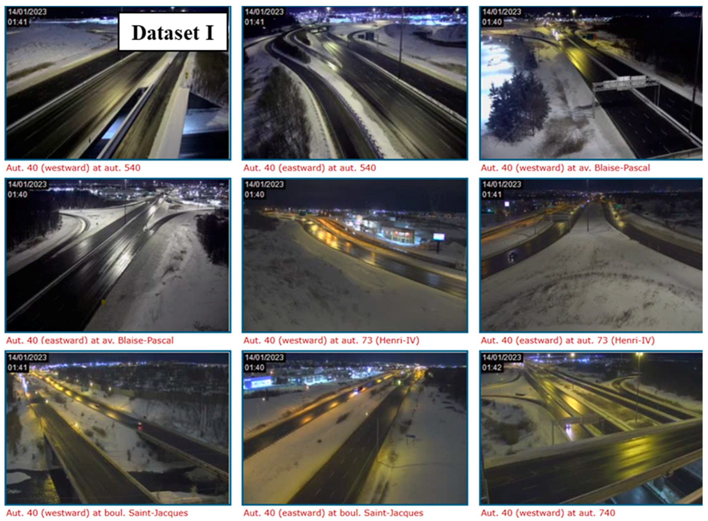
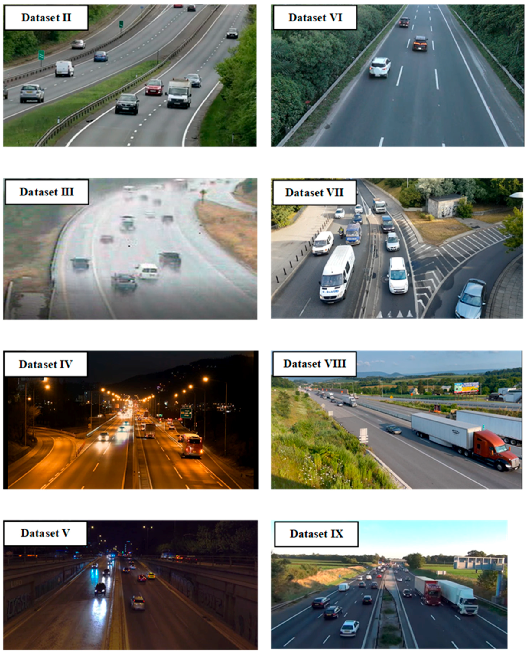
  • Providing the most challenging highway videos. To make an acceptable assessment, they must cover various states of vehicles, such as occlusion, weather conditions (i.e., rainy), low- to high-quality video frames, and different resolutions and illuminations (images collected during the day and at night). Also, the videos must be recorded from diverse viewing angles with cameras installed on top of road infrastructures, in order to determine the best locations. Section 2 covers this first contribution;
  • Making a comprehensive comparison between the deep learning algorithms in terms of acquiring accuracy in both vehicle detection and classification. The vehicles are categorized into the three classes of car, truck, and bus. The computation time of the algorithms is also assessed to determine which one presents a better potential usability in real-time situations. Section 3 covers this second contribution.

2. Traffic Video Data

The organization “Ministère des Transports et de la Mobilité durable du Québec”, located in the Province of Quebec, Canada, has established numerous online highway cameras. Figure 1 shows nine samples of images acquired with those cameras. The cameras work 24 h a day, covering multiple road lanes under all illumination and weather conditions. Therefore, these cameras are fairly suitable for use in our assessment of the deep learning structures relevant to vehicle detection and localization on highways. The vehicles appear relatively small on the images, which offer little contextual information due to the distance of the cameras from the road surface and the low resolution of the camera. The dimension of each frame is 352 × 240 , and the images were recorded on 14 January 2023.
In order to perform a comprehensive assessment of the methodologies, the processed highway videos should cover as many road challenges as possible. Therefore, the next high-quality image datasets were downloaded from YouTube and KAGGLE (www.kaggle.com, accessed on 12 September 2023) platforms (Figure 2). As can be seen in Figure 2, datasets IV and V include numerous vehicles, ranging from cars to buses, shown at night time. The main attribute of these two datasets is that the vehicles’ headlights are on, and the vehicles are moving fast in both directions. In other datasets, the cameras are relatively close to the cars on the roads, which results in the collection of more contextual information. Also, the angle of view of some of the cameras (i.e., dataset VII) is not perpendicular to the road infrastructure. This means that vehicles are recorded from a side view, and this increases the complexity of the environments considered. Shawon [38] released a video on KAGGLE, which is an online community platform for data scientists, in order to monitor traffic flow (dataset II). These cameras produce images with a resolution of 1364 × 768 pixels at a frequency of 25 FPS. This high-quality video includes various British vehicles ranging from commercial trucks to private cars. Another positive side of this video is that the vehicles therein move on two separate roads in opposite directions, meaning that the algorithms evaluate front and rear vehicle views. This video also provides more of the contextual information of on-road vehicles, which may enable better vehicle detection and classification. Another British highway dataset was released by Shah [39] including frequent challenging traffic flow types (Dataset III). Table 1 provides a summary of the information of the selected datasets in terms of pixel resolution, time of recording, etc. In the “Section 5.1”, we provide precise and in-depth explanations about why these datasets have been chosen.

3. Deep Learning Methodologies Applied to Vehicle Detection

The deep neural network structures generally comprise training data, region proposals, feature extraction, layer selection, and classifiers. Figure 3 presents an overview of a deep learning structure used for detecting and identifying a pattern or object in an image.
  • Training Data
Deep learning algorithms are mostly supervised and require pre-defined data, meaning that the images of vehicles, as the research focus of this study, should first be provided to the deep learning network. This process is undertaken by drawing boxes around each known object, such as in Figure 4a. As long as the training data are comprehensive and cover any vehicle state, ranging from color to type, the algorithm will detect vehicles precisely. In relation to this, various inclusive free-access datasets have been released; COCO (Common Objects in Common) and ILSVRC (Large Scale Visual Recognition Challenge) are two samples thereof. These are widely used as benchmark datasets in computer vision. They contain labeled images featuring diverse object categories, object annotations, and segmentation masks for object detection and recognition tasks. Figure 4b shows 400 pre-defined images from COCO, which include humans, animals, houses, and vehicles. In order to improve the amount of data and the model’s prediction accuracy, augmentation is suggested, which applies varying angular and rotation steps to the original data [41]. This also results in reducing the cost of labeling data, and generates variability and flexibility.
  • Region Proposals
Traditional algorithms have sought to assess individual pixels from the inputted images for the sake of object detection and localization. This process was shown to be time-consuming due to the required analysis of thousands of pixels by deep layer networks. The state-of-the-art methodologies represent several solutions to finding the candidate pixels, instead of evaluating pixel-by-pixel. For instance, the two SSD and YOLO methods divide the input images into grids of the same length. This process will reduce the computation time sharply as it analyzes only a few cells, instead of thousands of pixels. Assume image I has dimensions of 300 × 300 , and the grid of SSD is 8 × 8 . The computation process will be decreased from approximately 9 × 10 4   300 × 300 to 64.
  • Feature Extraction
Convolutional layers ( C o n v ) represent a popular feature extraction process because they can be used for calculating features without any human supervision. In addition, the convolutional layers prevent overfitting, which is a noticeable problem in machine learning algorithms, as they introduce flexibility in feature learning. A sample of feature extraction model VGG16 is shown in Figure 5a. Via trial and error, researchers have found the optimal convolution size, for example, 3 × 3 in SSD. Since these layers may feature negative values, an activation function is considered. Various activation functions (Equations (1)–(3)) have been proposed, and ReLU (Equation (1)) is an example thereof. The ReLU converts the negative values of the convolutional layers into zero. To reduce the huge volume of convolution layers, the two steps of max pooling and stride are required, as shown in Figure 5b.
ReLU :   f x = x x 0 0 x < 0
Sigmoid :   σ x = 1 1 + e x
Hyperbolic   Tangent :   T a n h = s i n h x c o s h x = e x e x e x + e x
where x is the value of the convolution layer’s outputs.
  • Layer Selection and Classifier
After feature extraction and pooling, the remaining features are flattered and fed into the deep-layer neurons. For each neuron, a feature is assigned. Afterward, a full connectivity ( F C ) neural network, which links a neuron to all the neurons in the adjacent layer, is considered. Next, a classifier, which can operate by machine learning, such as a Support Vector Machine (SVM) or a probabilistic model, is required to determine the object type. This classifier assigns a value of 0 ,   1 for each object of interest, whereby the image class has the highest score. To achieve the best performance in object detection and localization, a Back Propagation (BP) step is needed, which measures the weights between neurons and loss functions. The most popular loss functions are maximum likelihood, cross entropy, and Mean Squared Error (MSE) [43]. The loss function determines the difference between the predicted value of an image and its actual class. When the loss function reaches the minimum rate of difference, it is said that the deep learning algorithm works properly; in any other case, the algorithm’s structure should be changed and adjusted to ensure higher accuracy.
After setting out how a deep structure works, Figure 6 illustrates the flowcharts of SSD [26], RCNN [44], and YOLO [45] as the most popular vehicle detection methodologies. Each of these procedures features certain stages in the vehicle localization process, described as follows.

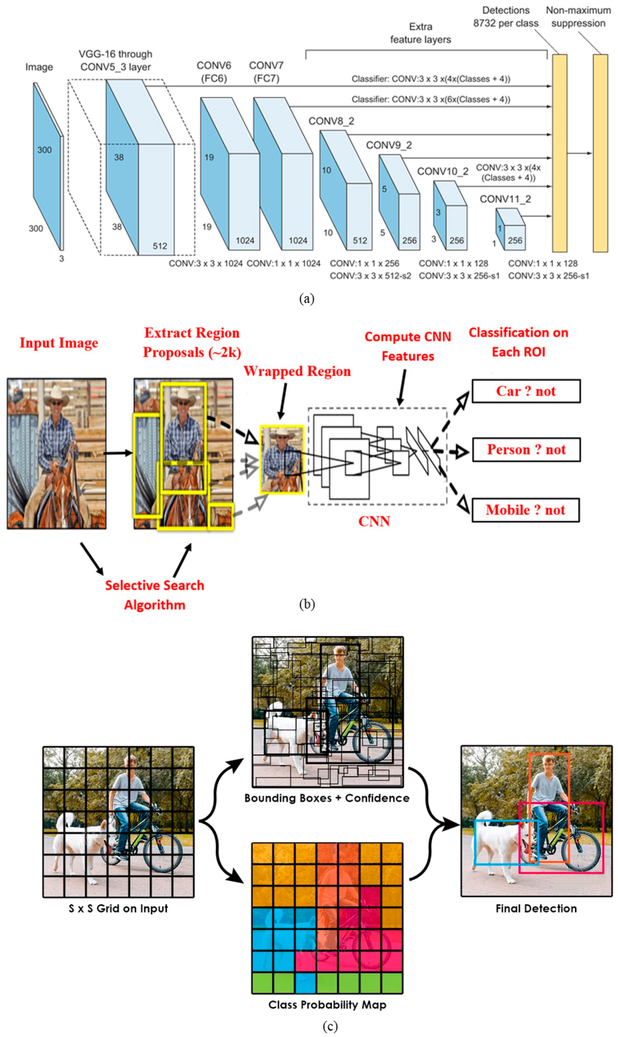
3.1. Single Shot Multi-Box Detector (SSD)

This algorithm was trained and evaluated on the two large free-access datasets Pascal VOC (Pattern Analysis, Statistical Modeling, and Computational Learning—Visual Object Classes) and COCO, and gained an mAP (mean average precision) score of more than 0.74%. SSD initially converts the inputted images, whether they comprise training or test data, into a feature map (grid) with a size of m × n (generally, the grid has dimensions of 8 × 8 ). Then, multiple boxes of different sizes are placed around each cell. The sizes and directions of these boxes are known. This is why it is called a multibox detector algorithm. Afterwards, features are measured with the help of VGG16 as the base network, due to its exceptional performance in classification and possession of several auxiliary convolutional layers. These features help in measuring multiple boxes’ scores between grids, and collecting ground truth data for each SSD class (i.e., vehicle, pedestrians).
The following equations (Equations (4)–(6)) show the process of score calculation for both ground truth boxes ( d ) and estimated ones ( l ) . Here, l   refers to the predicted boxes around each cell. Most corresponding ground truth boxes with l are detected by a matching strategy. The parameter of c is the class (i.e., vehicle, dog, cat, etc.), N is the number of boxes matched with l , and α is considered equal to one by cross-validation. Each box, whether ground truth or estimated, has four parameters of c e n t e r   o f   x   c x ,   c e n t e r   o f   y   c y ,   w i d t h   w   a n d   h e i g h t   h .
L x , c , l , g = 1 N L c o n f x , c + α L l o c x , l , g
L l o c x , l , g = i P o s N m c x , c y , w , h x i j k s m o o t h L 1 l i m g ^ j m g ^ j c x = g j c x d i c x d i w                                             g ^ j c y = g j c y d i c y d i h g ^ i w = log g j w d i w                                                 g ^ i h = log g j h d i h
L c o n f x , c = i P o s N x i j p log c ^ i p     where   c ^ i p = exp c i p p exp c i p

3.2. You Only Look Once (YOLO)

Like SSD, YOLO first converts the inputted data into S × S grids ( 7 × 7 ) of the same length and measure several bounding boxes around each grid cell (two boxes). Then, the five parameters of c x ,   c y ,   w , h and a c o n f i d e n c e   s c o r e are measured. The first four parameters represent the bounding box localization, but the c o n f i d e n c e   s c o r e refers to the maximum percentage of overlap between the YOLO bounding boxes and the ground truth boxes. This overlap is assessed by the Intersection Over Union (IOU) methodology, and its output is a probability value for each cell. If we consider the number of classes that YOLO can detect to be equal to 20, then 7 × 7 × 2 × 5 + 20 = 1470 values can be measured for each image. Afterwards, 26 convolutional layers are selected, of which the last two are fully connected. A 1 × 1 convolutional layer, like GoogleNet, is used for reducing the feature space. Notably, a tiny YOLO has also been released with nine convolutional layers, which is faster than YOLO. The final output of YOLO is a class probability, according to which a value between zero and one is assigned to each class. Therefore, the class with the highest value will be considered the class of the bounding box. As an image may contain no objects, boxes with a c o n f i d e n c e   s c o r e of near zero are eliminated, and are not considered in the next stages (this reduces the computation time). YOLO and tiny YOLO have achieved around 63% and 52% mAP accuracy, respectively, on the VOC 2007 dataset, but a 70% mAP accuracy when applied on VOC 2012. The main positive of this method is its ability to extract objects in 45 FPS (Frame Per Second), which means it is suitable for real-time object detection.
To date, eight versions of YOLO have been released for use in object extraction. YOLOv2 includes fine-grained features to improve the accuracy of detecting small objects [46]. Its capacity to detect small and multiscale objects was the main drawback of YOLOv1 [45]. Yolov3 uses logistic classifiers to assign a score to each class, while the previous ones used a SoftMax procedure [47]. YOLOv3 also employs Darknet-53 as the feature extraction step, with 53 convolutional layers, which is a deep neural network architecture commonly used for object detection and classification tasks. Increasing computation time and detecting object accuracy was the main aim of YOLOv4 [48]. It verified the negative effects of SOTA’s Bag-of-Freebies and Bag-of-Specials by use of COCO as the training dataset. YOLOv5 has a lower volume, around 27 MB, in comparison with YOLOv4 (277 MB), both of which were released in 2020 [49]. YOLOv6 showed that if an anchor-free procedure with Varifocal Length (VFL) is used throughout the training steps, the algorithm can run 51% faster than other anchor-based methods [50]. YOLOv7 mainly focused on generating accurate bounding boxes for detecting objects more precisely [51]. Recognizing objects quickly was the foremost goal of YOLOv8, which employed a cutting-edge SOTA model (www.ultralytics.com, accessed on 12 September 2023). This study will evaluate the four last versions of YOLO, i.e., 5, 6, 7, and 8, for use in vehicle detection from highway videos, because these versions are robust in detecting small objects and have optimized computation times.

3.3. Region-Based Convolutional Neural Network (RCNN)

The semantic segmentation (region proposals) of images is the first step of RCNN in the context of decreasing computation time [44]. The four similarities of texture, size, fill, and color are key to initial image segmentation. Afterward, Convolutional Neural Networks (CNN) are applied to each selected segment to extract its features. In this case of feature extraction, pre-trained CNN structures, such as ResNet, VGG19, and EfficientNet, can be used. Finally, multiple SVM procedures are trained to classify the extracted features as a specific object, like a vehicle. Fast-RCNN simultaneously applies a CNN structure to the whole of the inputted image and merges it with the region proposal [52]. This results in the extraction of more features from the region’s proposal segments. Faster RCNN uses a region proposal neural network structure instead of similarity conditions [53]. This selective search algorithm, based on neural networks, directly impacts the generation of high-quality region proposals. As the Faster RCNN does not use similarity conditions and is an end-to-end algorithm, the two versions of RCNN and Fast-RCNN are not addressed in this study.

4. Experimental Results

4.1. Accuracy Evaluation

This step provides numerical information on how many vehicles have been correctly detected. The Precision, Recall, and F1 Score accuracies are the most common aspects of algorithm evaluation [54]. The three parameters of True Positive (TP), False Positive (FP), and False Negative (FN) are required to measure accuracy. TP indicates the number of vehicles detected correctly by the algorithms, while FN shows the number of non-vehicles detected falsely as a vehicle. FP specifies the number of vehicles that have not been detected. The Precision accuracy, based on the equations below (Equations (7)–(9)), refers to how many vehicles in the datasets were detected properly, while Recall refers to what percentage of the algorithm’s output was vehicles. F1 Score is a performance metric that balances Precision and Recall.
In this stage, TP, FP, and FN are calculated for each individual frame, regardless of whether a vehicle appears in various adjacent frames. Noticeably, as images often include remote areas of a road wherein vehicles are rarely detected, a Region of Interest (RoI) selection stage is needed. The vehicles in dataset II yield acceptable contextual information, but the vehicles located in remote areas of dataset IV, for example, feature less appropriate information. Therefore, ROI is a suitable tool that can be used to assess the real performances of the deep learning algorithms in the context of vehicle detection and classification; thus, the sections of the videos wherein vehicles represent less than 5% of the frame size are not considered in the accuracy calculation because they offer little contextual information. As shown in Table 2, which summarizes the acquired results, YOLOv7 showed the best overall performance on nine datasets in terms of vehicle detection, with around 98% accuracy. The SSD and RCNN have not shown acceptable performances in the context of vehicle detection, with about 58% and less than 2%, respectively.
Precision = True   Positiv True   Positive + False   Positive = TP TP + FP × 100
Recall = True   Positiv True   Positive + False   Negative = TP TP + FN × 100
F 1 score = 2 × Precision × Recall Precision + Recall × 100

4.2. Localization Accuracy

The localization accuracy refers to how precisely the algorithms can estimate the positions of vehicles. The Root Mean Square Error (RMSE), as the most common method used in position evaluation, shows the amount of difference between the bounding box predicted with parameters of P c x , P c y , P w , P h and the ground truth bounding box G c x , G c y , G w , G h . As the ground truth datasets were unavailable, the bounding boxes around vehicles were drawn by an expert. The library of labels in the Python environment [55], a useful application for bounding box-drawing (called labeling), has been used because it is fast and user-friendly. In total, 200 vehicles were randomly selected, and we observed that the YOLO versions achieved the best performance when used for localization estimation, with RMSE values lower than 30 pixels. This value was more than 500 pixels for Faster RCNN. Between the YOLO versions, YOLOv8 showed a weaker performance in localization estimation. In the “Section 5.3”, we clearly compare the acquired and estimated localization accuracies between the methods.
R M S E i = i = 1 n G c x P c x 2 i + G c y P c y 2 i + G w P w 2 i + G h P h 2 i
where n is the number of bounding boxes considered in calculating the different localization accuracies between the estimations of the deep learning algorithms ( P ) and the ground truth (G). G c x   and   G c y are, respectively, the centers of the bounding box on the x-axis and y-axis, and G w , and   G h   are the width and height of the ground truth bounding boxes (G). This is also true for the bounding boxes estimated by the algorithms. P c x   and   P c y are, respectively, the centers of the bounding boxes on the x-axis and y-axis, and P w   and   P h are the width and height of the estimated bounding boxes (G).

4.3. Running Time

In terms of computational time, it is necessary to run the deep learning codes in similar environments to assess which algorithm achieves faster in vehicle detection. Here, we used a personal laptop computer system with the following specifications: Windows 10, RAM 16 G DDR3, Processors of Intel (R) Core (TM) i7-4700 HQ CPU @ 2.4 GHz. Python was used as the programming environment. During the processing of the deep learning code, other non-relevant apps, such as web browsers, that required RAM or CPU resources were turned off to avoid a slowdown of the processing time. Only the CPU was considered in the analysis of the processing time. Other processors, the RAM, and the Graphics Processing Unit (GPU) were neglected. It is worth mentioning that using GPU can sharply reduce the computation time and render the algorithms suitable for the real-time monitoring of roadway infrastructures. Assuming a camera records 30 frames per second (FPS = 30), an algorithm can be used in real-time monitoring if it extracts vehicles at less than 1/30 s = 0.033 s or 33 milliseconds (ms) from each frame. Figure 7 shows the computation times of YOLO versions and Faster RCNN on 1000 frames. As can be seen, YOLOv5 and YOLOv8 achieved the best performance, at around 100 ms, while Faster RCNN took about 2.5 s per frame. YOLOv7, which showed the best overall performance out of the nine datasets in vehicle detection, required around 800 ms per frame.

4.4. Vehicle Classification

The capacity to determine the class of each detected vehicle (i.e., private car, truck, bus) is a strength of the deep learning structures. This is because of the availability of free-access datasets such as COCO [56], which provide not only localization information using bounding boxes, but also the types of each of the objects. Section 4.1 shows how the deep learning algorithms work frame by frame, regardless of whether a vehicle appears in multiple consecutive frames [57].
In order to evaluate errors in the classification procedure, a confusion matrix is used. The parameters of the proposed confusion matrix can be seen in Table 3. This matrix has two axes corresponding to an object’s actual and predicted values. For example, the column of the car has three parameters of { P C C ,   P T C ,   P B C } , the sum of which equals the real number of vehicles in the region. But the row of cars { P C C ,   P C T ,   P C B } displays how many objects were detected as cars by the algorithms. The diagonal cells of { P C C ,   P T T ,   P B B } that have been highlighted in green are true positive values, representing correctly classified vehicles. The non-diagonal cells highlighted in orange are falsely classified vehicles. The following three parameters, Commission Error (CE), Overall Accuracy (OA), and Omission Error (OE), estimate the accuracy of the classification. Equations (11)–(17) show how the OA, CE, and OE parameters are measured to complete the confusion matrix. This algorithm performs best when the OA is near 100%, and the CE and OE are close to 0%. Table 4 displays the confusion matrix evaluated for each dataset, wherein the OA of each region is highlighted in grey. Similar to the vehicle detection results obtained in Section 4.1, the YOLOv7 algorithm again showed the best performance in object classification. In the Section 5.3, the acquired confusion matrixes are assessed in greater depth in order to better understand the algorithm’s performance.
Overall   Accuracy = P C C + P T T + P B B P C C + P C T + P C B + P T C + P T T + P T B + P B C + P B T + P B B × 100
C E C = P C T + P C B P C C + P C T + P C B × 100
C E T = P T C + P T B P T C + P T T + P T B × 100
C E B = P B C + P B T P B C + P B T + P B B × 100
O E C = P T C + P B C P C C + P T C + P B C × 100
O E T = P C T + P B T P C T + P T T + P B T × 100
O E B = P C B + P T B P C B + P T B + P B B × 100

5. Discussion

5.1. Datasets Challenges and Advantages

This section addresses the challenges the selected video datasets met in covering an important portion of the possible scenarios that could arise in traffic flow monitoring. These various and representative datasets can be used to evaluate cutting-edge deep learning vehicle detection algorithms more completely. First, illumination changes and shadow, as the most important challenge met by radiometric cameras due to their sensitivity to brightness, appear in datasets IV and V (Figure 8a,b). Secondly, a large variety of vehicles, ranging from private cars with diverse sizes and colors to large heavy vehicles such as buses, can be found in dataset VIII (Figure 8c) and dataset IV (Figure 8a). These vehicles can be found in several countries, such as Canada and England. Notably, a range of fields of view, set by different relations between the cameras and road surfaces (i.e., vertical, low oblique, high oblique), were considered as they provide different types of contextual information. For example, more vehicle bodies can be recorded by high oblique cameras (dataset VIII), while the top parts of vehicles can only be recorded by cameras with a vertical view (dataset VII) (Figure 8c,d).
Furthermore, the variation in scale of each individual vehicle is another challenge for the algorithms, which must be robust in this situation (Figure 8e,f). This variation is caused by the perspectives of cameras, meaning that an object near the camera will show a larger scale than more distant objects. The selected datasets also cover different weather conditions such as rainy and foggy to assess whether the algorithms can still detect vehicles (Figure 8g,h). Finally, vehicle occlusion, shown in Figure 8i, is another parameter that was covered by the datasets. The YOLOv7 algorithm seemed to work properly in such situations of unclear or inaccurate information.

5.2. Parameters Sensitivity

This section discusses various models of each YOLO version in terms of their computation time and acquired classification accuracy. The authors of the YOLO structures, unlike SSD or RCNN, released the five models of n ,   s ,   m ,   l , x , which have been sorted based on obtained accuracy and volume of parameters [28]. These models are generated via trial-and-error. Table 5 displays the model given by YOLOv8, with input values of image size—640 × 640, mean average precision (mAP), and parameter volume (million). The parameter volume includes network architecture, activation functions, learning rate, batch size, regularization techniques, and optimization algorithms. As can be seen, the YOLOv 8 n showed a faster performance on the COCO dataset, while the lowest accuracy in object classification. Although the model of YOLOv 8 x showed the greatest computation time and the best classification accuracy, we also tested this model on our dataset. We observed that it failed to improve vehicle detection accuracy in comparison to YOLOv8n, but also has the potential to extract false objects (Figure 9a). Since the real-time monitoring of vehicles is the main purpose of ITS, the model of {n} has been used across all YOLO versions. Figure 9b compares the YOLO versions, and we can see that YOLOv8 exhibited superior performance in COCO classification. However, our study demonstrates that YOLOv8 had a lower classification accuracy than YOLOv7 when applied to the highway datasets. To gain a deeper understanding of the parameters mentioned in Table 5 and the methods of calculating them, it is recommended to refer to the paper [58] for further insights.

5.3. Algorithms Comparison

This stage gives comparative information about the algorithms regarding vehicle detection, computation time, localization, and classification. Table 4 displays the accuracy acquired by the algorithms when applied to the nine selected datasets. As can be seen, YOLOv7 achieved the best vehicle detection accuracy, with a performance of 98.77%, while Faster RCNN and SSD showed the weakest performance, at about 50%. Also, the localization accuracy of Faster RCNN (Figure 10) and its computation time (Figure 7) were lower than those of the YOLO versions. According to our experimentation, Faster RCNN and SSD algorithms are unsuitable for use in highway vehicle detection. Except for dataset I, where YOLOv7 clearly showed the best detection performance, all YOLO versions have shown an acceptable vehicle detection performance above 90%. This means all YOLO versions work properly in day and nighttime, such as shown in dataset IV, reaching an accuracy above 98%. Also, all YOLO algorithms, especially YOLOv7, work properly in the diverse weather conditions presented in datasets I and III, with an accuracy of around 90%. In addition, our series of tests have demonstrated that the camera resolutions, angle of view (vertical, oblique, high oblique), diversity of vehicles, and even vehicle rear/front view have not negatively impacted the YOLO results. It is logical to conclude that the version YOLOv7 is the best vehicle detection and localization model. The recall accuracy of YOLOv7 was also the highest compared to the other models, while it was slower in terms of computation time.
One noteworthy observation is the remarkable performance of all YOLO versions, especially YOLOv7, when applied to nighttime datasets (dataset IV and dataset V). The results underscore YOLOv7’s exceptional capacity for accurately detecting vehicles during low light conditions, with an impressive accuracy exceeding 99%. Following closely, YOLOv8 also demonstrated a commendable performance, achieving an accuracy rate of approximately 98%. This outcome showcases the robustness and adaptability of these YOLO versions, shedding light on their potential applications in scenarios wherein darkness challenges visibility. These findings validate the efficacy of these models, and emphasize their relevance to real-world applications wherein nighttime surveillance and object detection are essential.
Following vehicle detection, a critical parameter for algorithm evaluation is the accuracy of classifying vehicles into car, truck, and bus categories. In this case, the OA (Equation (11)) parameter in Table 4 again shows that YOLOv7 was the best classifier, achieving a value of 97.37%, followed by YOLOv6 at 94.24%. Furthermore, the sums of errors of CE (Equations (12)–(14)) and OE (Equations (15)–(17)) were obtained per class in Table 4. As can be seen, private cars were more accurately detected, with the lowest errors of around 10%, while trucks and buses represented the greatest challenge in classification. The confusion matrix of dataset VIII presented in Table 4 shows the lowest rates of OE and CE errors. This is because oblique-view cameras capture more contextual information, which aids the algorithms in achieving superior classification.

5.4. Comparison with Previous Studies

We here introduce a novel method for comparing state-of-the-art vehicle detection algorithms. This comparison process makes us of challenging highway video datasets with various angles of view. These challenging datasets have not been addressed in previous studies, such as the one by Kim and Sung [30], which conducted a similar comparison between RCNN, SSD, and YOLO. They did not evaluate the algorithms in different illumination contexts, such as nighttime, and different weather conditions. Also, they customized the weights of each algorithm on their training data, which is time-consuming. Indeed, needing no additional training data is one benefit of our work. We suggest that future researchers use the primary model of each released algorithm for vehicle detection, without using any training data. Likewise, Song and Liang [59] used thousands of training data in customizing the weights of YOLO.
Similarly, Zhang, Hu [37] tried to enhance the performance of SSD for vehicle detection at night. Despite improving the SSD algorithm and achieving better detection and classification accuracy, its acquired accuracies (around 89%) are still lower than those of the YOLO versions (at about 98%). Neupane and Horanont [60] used the models produced by the YOLO versions as the base for transfer learning when enhancing training data, similarly to the previous works. In this case, they did not consider various cameras with different resolutions, or even illumination changes. Also, the enhanced YOLOs were not assessed in both night and daytime. A couple of studies on vehicle-board cameras have been published in the context of the evaluation of deep learning in vehicle detection [35,36]. Since these cameras have a completely different structures and fields of view from highway ones, this is not an effective way to compare the algorithms.
In conclusion, there is no need for additional training data to enhance the performance of YOLO versions in vehicle detection. The released versions of YOLO work effectively in vehicle detection and classification, without any considerable errors in localization. Heavy trucks are detected more accurately when the camera’s angle of view is oblique, while private cars are detectable with precision from any direction of view. Noticeably, the algorithm can be run in real-time situations if a GPU processor is used.

6. Conclusions and Future Works

In this paper, we have compared state-of-the-art deep learning algorithms, such as SSD, RCNN, and different versions of YOLO, for vehicle detection. These deep learning structures have been trained and tested on thousands of images acquired from highway cameras and contained in the COCO library. Nine video cameras facing potential challenges were selected for a fair and general comparison, covering a large spectrum of vehicle positions and shapes. These challenging datasets cover numerous angles of view between the camera and road, with different qualities of video (from both day and night) and variations in the scale of vehicles. The YOLO versions, particularly YOLOv7, achieved the best detection and localization accuracy, and the most accurate vehicle classification results for cars, trucks, and buses. In addition, the computation time of the YOLOs was under one-tenth of a second when using a CPU processor. This means the running time will be near real-time if GPU and RAM are used in addition to a CPU processor. With an accuracy in vehicle detection of about 98%, the YOLO versions can generally be used for ITS purposes such as real-time traffic flow monitoring.
In future research, it is strongly recommended to further evaluate deep learning architectures by application to Unmanned Aerial Vehicle (UAV) videos, which can encompass larger road areas. This will address the significant lack of accuracy in the classification of heavy vehicles, such as buses, which should be a priority. Furthermore, investigating the potential for the accurate localization and tracking of detected vehicles is crucial. These enhancements are anticipated to yield more realistic data for road traffic simulators.

Author Contributions

Conceptualization, D.S. and C.L.; methodology, D.S., C.L. and S.H.; software, D.S, C.L. and S.H.; validation, C.L. and S.H.; formal analysis, C.L. and S.H.; investigation, D.S.; resources, D.S.; data curation, D.S.; writing—original draft preparation, D.S.; writing—review and editing, C.L. and S.H.; visualization, D.S.; supervision, C.L. and S.H.; project administration, C.L.; funding acquisition, C.L. and S.H. All authors have read and agreed to the published version of the manuscript.

Funding

This research was funded by Mitacs grant number IT30935 and Semaphor.ai.

Data Availability Statement

Data sharing is not applicable to this paper.

Acknowledgments

The authors would like to thank all the individuals and organizations who made these datasets and algorithms available. In particular, we want to express our sincere appreciation and gratitude to the Semaphor.ai team and Mitacs for their funding support in making this project possible.

Conflicts of Interest

The authors declare no conflict of interest.

References

  1. Lv, Z.; Shang, W. Impacts of intelligent transportation systems on energy conservation and emission reduction of transport systems: A comprehensive review. Green Technol. Sustain. 2023, 1, 100002. [Google Scholar] [CrossRef]
  2. Pompigna, A.; Mauro, R. Smart roads: A state of the art of highways innovations in the Smart Age. Eng. Sci. Technol. Int. J. 2022, 25, 100986. [Google Scholar] [CrossRef]
  3. Regragui, Y.; Moussa, N. A real-time path planning for reducing vehicles traveling time in cooperative-intelligent transportation systems. Simul. Model. Pract. Theory 2023, 123, 102710. [Google Scholar] [CrossRef]
  4. Wu, Y.; Wu, L.; Cai, H. A deep learning approach to secure vehicle to road side unit communications in intelligent transportation system. Comput. Electr. Eng. 2023, 105, 108542. [Google Scholar] [CrossRef]
  5. Zuo, J.; Dong, L.; Yang, F.; Guo, Z.; Wang, T.; Zuo, L. Energy harvesting solutions for railway transportation: A comprehensive review. Renew. Energy 2023, 202, 56–87. [Google Scholar] [CrossRef]
  6. Yang, Z.; Peng, J.; Wu, L.; Ma, C.; Zou, C.; Wei, N.; Zhang, Y.; Liu, Y.; Andre, M.; Li, D.; et al. Speed-guided intelligent transportation system helps achieve low-carbon and green traffic: Evidence from real-world measurements. J. Clean. Prod. 2020, 268, 122230. [Google Scholar] [CrossRef]
  7. Chen, Z.; Guo, H.; Yang, J.; Jiao, H.; Feng, Z.; Chen, L.; Gao, T. Fast vehicle detection algorithm in traffic scene based on improved SSD. Measurement 2022, 201, 111655. [Google Scholar] [CrossRef]
  8. Ribeiro, D.A.; Melgarejo, D.C.; Saadi, M.; Rosa, R.L.; Rodríguez, D.Z. A novel deep deterministic policy gradient model applied to intelligent transportation system security problems in 5G and 6G network scenarios. Phys. Commun. 2023, 56, 101938. [Google Scholar] [CrossRef]
  9. Sirohi, D.; Kumar, N.; Rana, P.S. Convolutional neural networks for 5G-enabled Intelligent Transportation System: A systematic review. Comput. Commun. 2020, 153, 459–498. [Google Scholar] [CrossRef]
  10. Lackner, T.; Hermann, J.; Dietrich, F.; Kuhn, C.; Angos, M.; Jooste, J.L.; Palm, D. Measurement and comparison of data rate and time delay of end-devices in licensed sub-6 GHz 5G standalone non-public networks. Procedia CIRP 2022, 107, 1132–1137. [Google Scholar] [CrossRef]
  11. Wang, Y.; Cao, G.; Pan, L. Multiple-GPU accelerated high-order gas-kinetic scheme for direct numerical simulation of compressible turbulence. J. Comput. Phys. 2023, 476, 111899. [Google Scholar] [CrossRef]
  12. Sharma, H.; Kumar, N. Deep learning based physical layer security for terrestrial communications in 5G and beyond networks: A survey. Phys. Commun. 2023, 57, 102002. [Google Scholar] [CrossRef]
  13. Ounoughi, C.; Ben Yahia, S. Data fusion for ITS: A systematic literature review. Inf. Fusion 2023, 89, 267–291. [Google Scholar] [CrossRef]
  14. Afat, S.; Herrmann, J.; Almansour, H.; Benkert, T.; Weiland, E.; Hölldobler, T.; Nikolaou, K.; Gassenmaier, S. Acquisition time reduction of diffusion-weighted liver imaging using deep learning image reconstruction. Diagn. Interv. Imaging 2023, 104, 178–184. [Google Scholar] [CrossRef] [PubMed]
  15. Xu, M.; Yoon, S.; Fuentes, A.; Park, D.S. A Comprehensive Survey of Image Augmentation Techniques for Deep Learning. Pattern Recognit. 2023, 137, 109347. [Google Scholar] [CrossRef]
  16. Zhou, Y.; Ji, A.; Zhang, L.; Xue, X. Sampling-attention deep learning network with transfer learning for large-scale urban point cloud semantic segmentation. Eng. Appl. Artif. Intell. 2023, 117, 105554. [Google Scholar] [CrossRef]
  17. Yu, C.; Zhang, Z.; Li, H.; Sun, J.; Xu, Z. Meta-learning-based adversarial training for deep 3D face recognition on point clouds. Pattern Recognit. 2023, 134, 109065. [Google Scholar] [CrossRef]
  18. Kim, C.; Ahn, S.; Chae, K.; Hooker, J.; Rogachev, G. Noise signal identification in time projection chamber data using deep learning model. Nucl. Instrum. Methods Phys. Res. Sect. A Accel. Spectrometers Detect. Assoc. Equip. 2023, 1048, 168025. [Google Scholar] [CrossRef]
  19. Zhang, X.; Zhai, D.; Li, T.; Zhou, Y.; Lin, Y. Image inpainting based on deep learning: A review. Inf. Fusion 2023, 90, 74–94. [Google Scholar] [CrossRef]
  20. Mo, W.; Zhang, W.; Wei, H.; Cao, R.; Ke, Y.; Luo, Y. PVDet: Towards pedestrian and vehicle detection on gigapixel-level images. Eng. Appl. Artif. Intell. 2023, 118, 105705. [Google Scholar] [CrossRef]
  21. Bie, M.; Liu, Y.; Li, G.; Hong, J.; Li, J. Real-time vehicle detection algorithm based on a lightweight You-Only-Look-Once (YOLOv5n-L) approach. Expert Syst. Appl. 2023, 213, 119108. [Google Scholar] [CrossRef]
  22. Liang, Z.; Huang, Y.; Liu, Z. Efficient graph attentional network for 3D object detection from Frustum-based LiDAR point clouds. J. Vis. Commun. Image Represent. 2022, 89, 103667. [Google Scholar] [CrossRef]
  23. Tian, Y.; Guan, W.; Li, G.; Mehran, K.; Tian, J.; Xiang, L. A review on foreign object detection for magnetic coupling-based electric vehicle wireless charging. Green Energy Intell. Transp. 2022, 1, 100007. [Google Scholar] [CrossRef]
  24. Yang, Z.; Pun-Cheng, L.S. Vehicle detection in intelligent transportation systems and its applications under varying environments: A review. Image Vis. Comput. 2018, 69, 143–154. [Google Scholar] [CrossRef]
  25. Wang, Z.; Ma, Y.; Zhang, Y. Review of pixel-level remote sensing image fusion based on deep learning. Inf. Fusion 2023, 90, 36–58. [Google Scholar] [CrossRef]
  26. Liu, W.; Anguelov, D.; Erhan, D.; Szegedy, C.; Reed, S.; Fu, C.Y.; Berg, A.C. SSD: Single Shot MultiBox Detector. In Computer Vision and Pattern Recogniti; Springer International Publishing: Cham, Switzerland, 2016. [Google Scholar]
  27. Girshick, R.; Donahue, J.; Darrell, T.; Malik, J. Region-Based Convolutional Networks for Accurate Object Detection and Segmentation. IEEE Trans. Pattern Anal. Mach. Intell. 2016, 38, 142–158. [Google Scholar] [CrossRef]
  28. Jiang, P.; Ergu, D.; Liu, F.; Cai, Y.; Ma, B. A Review of Yolo Algorithm Developments. Procedia Comput. Sci. 2022, 199, 1066–1073. [Google Scholar] [CrossRef]
  29. Ramachandran, A.; Sangaiah, A.K. A review on object detection in unmanned aerial vehicle surveillance. Int. J. Cogn. Comput. Eng. 2021, 2, 215–228. [Google Scholar] [CrossRef]
  30. Kim, J.A.; Sung, J.Y.; Park, S.H. Comparison of Faster-RCNN, YOLO, and SSD for Real-Time Vehicle Type Recognition. In Proceedings of the 2020 IEEE International Conference on Consumer Electronics—Asia (ICCE-Asia), Seoul, Republic of Korea, 1–3 November 2020. [Google Scholar]
  31. Qiu, Q.; Lau, D. Real-time detection of cracks in tiled sidewalks using YOLO-based method applied to unmanned aerial vehicle (UAV) images. Autom. Constr. 2023, 147, 104745. [Google Scholar] [CrossRef]
  32. Dang, F.; Chen, D.; Lu, Y.; Li, Z. YOLOWeeds: A novel benchmark of YOLO object detectors for multi-class weed detection in cotton production systems. Comput. Electron. Agric. 2023, 205, 107655. [Google Scholar] [CrossRef]
  33. Li, M.; Zhang, Z.; Lei, L.; Wang, X.; Guo, X. Agricultural Greenhouses Detection in High-Resolution Satellite Images Based on Convolutional Neural Networks: Comparison of Faster R-CNN, YOLO v3 and SSD. Sensors 2020, 20, 4938. [Google Scholar] [CrossRef] [PubMed]
  34. Azimjonov, J.; Özmen, A. A real-time vehicle detection and a novel vehicle tracking systems for estimating and monitoring traffic flow on highways. Adv. Eng. Inform. 2021, 50, 101393. [Google Scholar] [CrossRef]
  35. Han, X.; Chang, J.; Wang, K. Real-time object detection based on YOLO-v2 for tiny vehicle object. Procedia Comput. Sci. 2021, 183, 61–72. [Google Scholar] [CrossRef]
  36. Tao, C.; He, H.; Xu, F.; Cao, J. Stereo priori RCNN based car detection on point level for autonomous driving. Knowl. -Based Syst. 2021, 229, 107346. [Google Scholar] [CrossRef]
  37. Zhang, Q.; Hu, X.; Yue, Y.; Gu, Y.; Sun, Y. Multi-object detection at night for traffic investigations based on improved SSD framework. Heliyon 2022, 8, e11570. [Google Scholar] [CrossRef]
  38. Shawon, A. Road Traffic Video Monitoring. 2020. Available online: https://www.kaggle.com/datasets/shawon10/road-traffic-video-monitoring?select=traffic_detection.mp4 (accessed on 1 January 2021).
  39. Shah, A. Highway Traffic Videos Dataset. 2020. Available online: https://www.kaggle.com/datasets/aryashah2k/highway-traffic-videos-dataset (accessed on 1 March 2020).
  40. Saha, S. A Comprehensive Guide to Convolutional Neural Networks—The ELI5 Way. 2018. Available online: https://towardsdatascience.com/a-comprehensive-guide-to-convolutional-neural-networks-the-eli5-way-3bd2b1164a53 (accessed on 15 December 2018).
  41. Ding, J.; Li, X.; Kang, X.; Gudivada, V.N. Augmentation and evaluation of training data for deep learning. In Proceedings of the 2017 IEEE International Conference on Big Data (Big Data), Boston, MA, USA, 11–14 December 2017. [Google Scholar]
  42. Phuong, T.M.; Diep, N.N. Speeding Up Convolutional Object Detection for Traffic Surveillance Videos. In Proceedings of the 2018 10th International Conference on Knowledge and Systems Engineering (KSE), Ho Chi Minh City, Vietnam, 1–3 November 2018. [Google Scholar]
  43. Tian, Y.; Su, D.; Lauria, S.; Liu, X. Recent advances on loss functions in deep learning for computer vision. Neurocomputing 2022, 497, 129–158. [Google Scholar] [CrossRef]
  44. Girshick, R.; Donahue, J.; Darrell, T.; Malik, J. Rich feature hierarchies for accurate object detection and semantic segmentation. In Proceedings of the IEEE Conference on Computer Vision and Pattern Recognition, Columbus, OH, USA, 23–28 June 2014. [Google Scholar]
  45. Redmon, J.; Divvala, S.; Girshick, R.; Farhadi, A. You Only Look Once: Unified, Real-Time Object Detection. In Proceedings of the 2016 IEEE Conference on Computer Vision and Pattern Recognition (CVPR), Las Vegas, NV, USA, 27–30 June 2016. [Google Scholar]
  46. Redmon, J.; Farhadi, A. YOLO9000: Better, Faster, Stronger. In Proceedings of the 2017 IEEE Conference on Computer Vision and Pattern Recognition (CVPR), Honolulu, HI, USA, 21–26 July 2017. [Google Scholar]
  47. Redmon, J.; Farhadi, A. Yolov3: An incremental improvement. arXiv 2018, arXiv:1804.02767. [Google Scholar]
  48. Bochkovskiy, A.; Wang, C.-Y.; Liao, H.-Y.M. Yolov4: Optimal speed and accuracy of object detection. arXiv 2020, arXiv:2004.10934. [Google Scholar]
  49. Jocher, G. Yolov5. Code Repository. 2020. Available online: https://github.com/ultralytics/yolov5 (accessed on 1 July 2020).
  50. Li, C.; Li, L.; Jiang, H.; Weng, K.; Geng, Y.; Li, L.; Ke, Z.; Li, Q.; Cheng, M.; Nie, W.; et al. YOLOv6: A single-stage object detection framework for industrial applications. arXiv 2022, arXiv:2209.02976. [Google Scholar]
  51. Wang, C.-Y.; Bochkovskiy, A.; Liao, H.-Y.M. YOLOv7: Trainable bag-of-freebies sets new state-of-the-art for real-time object detectors. arXiv 2022, arXiv:2207.02696. [Google Scholar]
  52. Girshick, R. Fast r-cnn. In Proceedings of the IEEE International Conference on Computer Vision, Santiago, Chile, 7–13 December 2015. [Google Scholar]
  53. Chen, X.; Gupta, A. An implementation of faster rcnn with study for region sampling. arXiv 2017, arXiv:1702.02138. [Google Scholar]
  54. Powers, D.M. Evaluation: From precision, Recall and F-measure to ROC, informedness, markedness and correlation. arXiv 2020, arXiv:2010.16061. [Google Scholar]
  55. Vostrikov, A.; Chernyshev, S. Training sample generation software. In Intelligent Decision Technologies 2019, Proceedings of the 11th KES International Conference on Intelligent Decision Technologies (KES-IDT 2019), St. Julians, Malta, 17–19 June 2019; Springer: Berlin/Heidelberg, Germany, 2019; Volume 2. [Google Scholar]
  56. Lin, T.Y.; Maire, M.; Belongie, S.; Hays, J.; Perona, P.; Ramanan, D.; Dollár, P.; Zitnick, C.L. Microsoft coco: Common objects in context. In Computer Vision–ECCV 2014, Proceedings of the 13th European Conference, Zurich, Switzerland, 6–12 September 2014, Part V 13; Springer: Berlin/Heidelberg, Germany, 2014. [Google Scholar]
  57. Bathija, A.; Sharma, G. Visual object detection and tracking using Yolo and sort. Int. J. Eng. Res. Technol. 2019, 8, 705–708. [Google Scholar]
  58. Terven, J.; Cordova-Esparza, D. A comprehensive review of YOLO: From YOLOv1 to YOLOv8 and beyond. arXiv 2023, arXiv:2304.00501. [Google Scholar]
  59. Song, H.; Liang, H.; Li, H.; Dai, Z.; Yun, X. Vision-based vehicle detection and counting system using deep learning in highway scenes. Eur. Transp. Res. Rev. 2019, 11, 51. [Google Scholar] [CrossRef]
  60. Neupane, B.; Horanont, T.; Aryal, J. Real-Time Vehicle Classification and Tracking Using a Transfer Learning-Improved Deep Learning Network. Sensors 2022, 22, 3813. [Google Scholar] [CrossRef] [PubMed]
Figure 1. Samples of highway cameras located in Quebec, Canada.
Smartcities 06 00134 g001
Figure 2. Views of the selected video datasets used for the evaluation of the deep learning structures.
Smartcities 06 00134 g002
Figure 3. An overview of a deep learning structure [40].
Smartcities 06 00134 g003
Figure 4. Training data in order to feed them into deep learning structures [42]; (a) bounding boxes around vehicles, (b) samples from the COCO dataset used as training data (www.coco.org, accessed on 12 September 2023).
Smartcities 06 00134 g004
Figure 5. Feature extraction: (a) the VGG16 model used for feature extraction (www.towardsdatascience.com, accessed on 12 September 2023); (b) applying pooling and stride to a 4 × 4 image (www.geeksforgeeks.org, accessed on 12 September 2023).
Smartcities 06 00134 g005
Figure 6. Deep learning structures of (a) SSD [26], (b) RCNN [44], and (c) YOLO [45].
Smartcities 06 00134 g006
Figure 7. The computation times of YOLO versions and Faster RCNN over 1000 frames.
Smartcities 06 00134 g007
Figure 8. Datasets’ challenges; (a,b) illumination and shadow; (c,d) high oblique and low oblique angles of view; (e,f) scale variation of vehicles; (g,h) weather conditions such as foggy and rainy; (i) detection of vehicles that were occluded.
Smartcities 06 00134 g008
Figure 9. Parameter sensitivity of YOLO models: (a) outputs of two models of YOLO8; (b) comparison of YOLO models in terms of parameters’ volume and acquired accuracies.
Smartcities 06 00134 g009
Figure 10. Localization accuracy of (a) YOLO and (b) Faster RCNN algorithms.
Smartcities 06 00134 g010
Table 1. Specification attributes of the selected datasets.
DatasetDay/NightFramesFPSHeightWidthRear/FrontQualityAngle of View (AoV)Link (accessed on 12 September 2023)
Dataset IBoth225015352240BothLowVertical-Low-Highhttps://www.quebec511.info/fr/Carte/Default.aspx
Dataset IIDay1525251364768BothMediumLowhttps://www.kaggle.com/datasets/shawon10/road-traffic-video-monitoring
Dataset IIIDay25010320240RearLowVerticalhttps://www.kaggle.com/datasets/aryashah2k/highway-traffic-videos-dataset
Dataset IVNight61,840301280720BothVery HighVerticalhttps://www.youtube.com/watch?v=xEtM1I1Afhc
Dataset VNight178,125251280720BothLowVerticalhttps://www.youtube.com/watch?v=iA0Tgng9v9U
Dataset VIDay62,72730854480RearMediumVerticalhttps://youtu.be/QuUxHIVUoaY
Dataset VIIDay91803019201080FrontVery HighLowhttps://www.youtube.com/watch?v=MNn9qKG2UFI&t=7s
Dataset VIIIDay107,922301280720FrontHighHighhttps://youtu.be/TW3EH4cnFZo
Dataset IXDay1525251280720BothHighVerticalhttps://www.youtube.com/watch?v=wqctLW0Hb_0&t=10s
Table 2. Results acquired by the deep learning structures applied to nine datasets.
Yolov8Yolov7Yolov6Yolov5Faster RCNNSSD
Dataset IPrecision43.0396.3348.9654.982.00<2.00<
Recall55.41100.0078.3965.402.00<2.00<
F1-score48.4498.1360.2759.742.00<2.00<
Dataset IIPrecision99.38100.00100.00100.0092.492.00<
Recall100.00100.0096.7899.11100.002.00<
F1-score99.69100.0098.3699.5596.102.00<
Dataset IIIPrecision87.8497.3698.2596.742.00<2.00<
Recall83.56100.0099.69100.002.00<2.00<
F1-score85.6598.6698.9698.342.00<2.00<
Dataset IVPrecision98.42100.00100.00100.0037.242.00<
Recall99.6899.4796.5496.5598.442.00<
F1-score99.0599.7398.2498.2454.042.00<
Dataset VPrecision96.3397.7795.8794.382.00<2.00<
Recall97.9698.6993.1496.732.00<2.00<
F1-score97.1498.2394.4995.542.00<2.00<
Dataset VIPrecision100.00100.0099.18100.0088.922.00<
Recall96.5799.98100.0099.23100.002.00<
F1-score98.2699.9999.5999.6194.142.00<
Dataset VIIPrecision99.8299.8598.67100.0097.572.00<
Recall78.3686.1480.2285.6498.612.00<
F1-score87.8092.4988.4992.2698.092.00<
Dataset VIIIPrecision96.2899.4397.6599.4496.732.00<
Recall56.47100.0080.2597.8299.372.00<
F1-score71.1999.7188.1098.6298.032.00<
Dataset IXPrecision100.0098.2398.0099.1173.292.00<
Recall93.6698.3784.3699.8685.372.00<
F1-score96.7398.3091.5299.4878.872.00<
AveragePrecision91.2398.7792.9593.8554.692.00<
Recall84.6398.0789.9393.3765.312.00<
F1-score87.1098.4291.4293.6158.362.00<
Table 3. Parameters of a confusion matrix used for classification accuracy evaluation.
Actual
CarTruckBusCommission Error
PredictedCar P C C P C T P C B C E C
Truck P T C P T T P T B C E T
Bus P B C P B T P B B C E B
Omission Error O E C O E T O E B Overall Accuracy
Table 4. Confusion matrix of YOLO versions used for the evaluation of vehicle classification. A grey color is used to highlight the OA.
Yolov8 Yolov7 Yolov6 Yolov5
CarTruckBus CarTruckBus CarTruckBus CarTruckBus
Car1151209.45255301.16131604.38144604.00
Dataset ITruck314017.65729019.44322012.001217041.38
Bus000N/A000N/A000N/A030N/A
2.5446.15N/A88.972.679.38N/A96.602.2421.43N/A94.447.6934.62N/A89.94
Car63000.0063000.0062304.6260000.00
Dataset IITruck01000.0001100.0018011.11311021.43
Bus010N/A000N/A000N/A000N/A
d 0.009.09N/A98.650.000.00N/A100.001.5927.27N/A94.594.760.00N/A95.95
Car50407.4159101.6751407.27496010.91
Dataset IIITruck210016.67211015.38311021.4311207.69
Bus230N/A000N/A010N/A340N/A
7.4141.18N/A84.513.288.33N/A95.895.5626.67N/A88.577.5545.45N/A81.33
Car140566175.5814025574.23141062145.1114086064.48
Dataset IVTruck9264168.6512284117.496276157.078272188.72
Bus0182740.00094217.650103124.390163630.77
0.6423.2655.0093.080.8518.3930.0094.840.4220.6948.3394.130.5621.8440.0094.08
Car2758210.112758200.072758300.111750200.11
Dataset VTruck06114.2906114.2905228.5766114.29
Bus0030.000040.000030.000040.00
0.0025.0040.0099.860.0020.0020.0099.890.0037.5040.0099.820.3425.0020.0099.49
Car4941302.565031102.144961302.554811603.22
Dataset VITruck4472037.933576031.533969036.115771044.53
Bus09564.2907558.33010566.6707558.33
8.1823.400.0089.646.5119.150.0091.687.2925.000.0090.1910.5924.470.0087.44
Car1831306.63282301.05237602.47245602.39
Dataset VIITruck1729036.9656107.581150018.031348021.31
Bus872343.5101420.0039947.692911490.91
36.2455.380.0060.671.744.690.0097.4717.4223.080.0091.8014.6326.150.0090.83
Car4382004.37438000.00438000.00438000.00
Dataset VIIITruck05800.00026800.00026300.00026600.00
Bus02140N/A000N/A050N/A020N/A
0.0079.86N/A67.950.000.00N/A100.000.001.87N/A99.290.000.75N/A99.72
Car149201.32152000.00151704.43150805.06
Dataset IXTruck314017.6501900.0011207.6929018.18
Bus030N/A000N/A000N/A020N/A
1.9726.32N/A95.320.000.00N/A100.000.6636.84N/A95.321.3252.63N/A92.98
Table 5. Summary of YOLOv8 models.
ModelSize (Pixels)mAPvalSpeed CPU ONNXSpeed A100 Tensor RTParams (M)FLOPs
YOLOv8n64037.380.40.993.28.7
YOLOv8s64044.9128.41.2011.228.6
YOLOv8m64050.2234.71.8325.978.9
YOLOv8l64052.9375.22.3943.7165.2
YOLOv8x64053.9479.13.5368.2257.8
Disclaimer/Publisher’s Note: The statements, opinions and data contained in all publications are solely those of the individual author(s) and contributor(s) and not of MDPI and/or the editor(s). MDPI and/or the editor(s) disclaim responsibility for any injury to people or property resulting from any ideas, methods, instructions or products referred to in the content.

