Article

Prediction and Evaluation of Electricity Price in Restructured Power Systems Using Gaussian Process Time Series Modeling

by
Abdolmajid Dejamkhooy
* and
Ali Ahmadpour
Department of Electrical Engineering, University of Mohaghegh Ardabili, Ardabil 56199-11367, Iran
*
Author to whom correspondence should be addressed.
Smart Cities 2022, 5(3), 889-923; https://doi.org/10.3390/smartcities5030045
Submission received: 17 May 2022 / Revised: 29 June 2022 / Accepted: 27 July 2022 / Published: 5 August 2022
(This article belongs to the Topic Electricity Demand-Side Management)

Abstract

:
The electricity market is particularly complex due to the different arrangements and structures of its participants. If the energy price in this market presents in a conceptual and well-known way, the complexity of the market will be greatly reduced. Drastic changes in the supply and demand markets are a challenge for electricity prices (EPs), which necessitates the short-term forecasting of EPs. In this study, two restructured power systems are considered, and the EPs of these systems are entirely and accurately predicted using a Gaussian process (GP) model that is adapted for time series predictions. In this modeling, various models of the GP, including dynamic, static, direct, and indirect, as well as their mixture models, are used and investigated. The effectiveness and accuracy of these models are compared using appropriate evaluation indicators. The results show that the combinations of the GP models have lower errors than individual models, and the dynamic indirect GP was chosen as the best model.

1. Introduction

1.1. Motivation

Electricity is an essential and critical need at all application levels. The inability of technologies to store this energy on a large scale has made it more difficult for operation plans. Therefore, the production of the electricity price (EP) in supply and demand is a challenge in the electricity industry and markets [1]. The EP has a direct relationship with the amount of consumed load, and all economic planning and management of utilities depend on this relationship [2]. Moreover, the existence of regular and committed policies in development plans should be considered. For instance, reliability is one of the tasks of generation units, which along with other policies, such as environmental protection and the development of appropriate infrastructure for the use of renewable energy, is so effective in the quality of delivered energy [3]. For this purpose, optimal planning in the restructured power systems is divided into three parts in terms of time, including the long term (more than 10 years), the medium term (1 year), the short term (1 week to 1 month), and instant planning (from 1 min to a few hours) [4]. In these plans, some data should be used, such as load consumption and EPs, taking into account economic conditions and the average annual EP. Additionally, another important parameter is the size of the demand load, which is a nonlinear function of time and is studied daily (day or night), seasonally (hot or cold), and with regard to climatic conditions of the region [5]. Electricity with different structures and capabilities is always supplied and demanded in the electricity market. Therefore, a competitive market in the field of production to consumption will be created [6]. The reason for this competition can be summarized in the fact that electricity cannot be stored. In other words, there is no shortage or excess of energy in a power system that can be stored or consumed. On the other hand, the instability of the EPs results in more complications in energy markets [7]. As a result, different patterns and levels of electricity demand will be created that are highly time-dependent (at least hourly). Each of the mentioned periods contains valuable features that enhance management effectiveness. Among these periods, short-term forecasting has the greatest effect on electricity pricing [5,6]. The most important advantage of short-term forecasting is that it increases the quality of supply and demand offers. Consequently, choosing the most accurate method, and at the same time quickly, for the prediction of EPs is a significant and necessary issue.

1.2. Related Works

Short-term forecasting methods, which are the main goal of this study, can be divided into two main categories. The first category contains the fitting analysis, and the second category contains expert systems, Kalman filters, neural networks, and neural networks combined with fuzzy systems. Each of these methods performed in various research has drawbacks and advantages in the accuracy or proper analysis of the defined variables. In other classifications, the prediction models could be grouped into three classes: statistical, artificial intelligence, and combined methods.
In [8], a comprehensive review of various methods for forecasting EP has been investigated. A hybrid EP forecasting model based on the chaotic sine–cosine algorithm and the isolation forest algorithm is used in [9]. In other studies, hybrid models consist of various combinations, and modified methods of the auto-regressive integrated moving average (ARIMA) are proposed for the short-term forecasting of EP [10,11,12]. The statistical manners could consist of Bayesian [13], vector auto-regression [14], and Kalman filters [15]. Artificial intelligence algorithms (AIAs) are better than statistical methods because the AIAs can obtain the nonlinear characteristics and fast variations of the variables [1].
There are several types of research for EP forecasting that use various forms of AIAs, such as different models of the artificial neural network (ANN) [16,17,18,19,20], extreme learning machine (ELM) [21], and support vector machine (SVM) [22]. In [22], an advanced structure of neural networks is used for the prediction of the EP based on the repetition of the production of multilayer neural networks. In a recent study [1], the improved multi-objective sine–cosine algorithm was able to improve electricity market management in addition to the prediction of the EPs. The multi-structured improved neural network method has been proposed in [23], which is able to estimate the EP well and has shown to be more effective than other conventional ANNs. In [24], a novel hybrid future selector in smart grids is proposed based on the SVM, and then, a new model for predicting the EP is presented using the differential evolution algorithm (DEA).
Conventional individual models cannot extract the whole main characteristics of the EPs. Some hybrid methods are studied in several types of research that are pointed out in this section. In [25], a hybrid manner using the gravitational search algorithm, SVM, and wavelet transform (WT) is created for EP prediction in the electricity markets. In a similar work, the WT and ELM are combined for EP forecasting [26]. The authors of [27] proposed a hybrid model using WT, modified ANN, and generalized autoregressive conditional heteroskedasticity (GARCH) for the prediction of EP in the Spanish electricity market. The decomposition methods are developed for data mining applications and have been employed for several predictions in various fields. Wind power [28,29] and electrical load [2,30] are examples of these methods.
The time series models have been employed in several forecasting applications. These models can be classed into four main groups as follows:
  • WT decomposition models: These models can decompose the main data of the problem into sub-data that contain various frequencies. Therefore, the outputs with low errors are extracted in the time domain. However, the WT model has a weakness as it needs more prior data for various decomposition levels [1]. Additionally, this model has few applications because it is a non-compatible approach [31].
  • Singular Spectrum Analysis (SSA): this method eliminates the noises from the time series data [32], but its parameters are difficult to set or optimize. In other words, when the each of parameters was modified, the precision of the forecasting changed.
  • Empirical Mode Decomposition (EMD): this algorithm in the original mode needs low hyper-parameters (HPs) that can find the local oscillations in the main data [33].
  • Variational Mode Decomposition (VMD): this method is better than the three previous methods because of low data mining, easy modification of parameters, and better findings in the local oscillations, as reported in various studies [1,9,34]. However, this method cannot obtain acceptable accuracy in forecasting.
As mentioned in the above-summarized cases, the forecasting of any data needs faster, lower parameters, and a more accurate method for enhancing the performance of systems. The Gaussian process (GP), as reported in several kinds of research [35,36,37,38], could overcome the above problems. For example, in [35], the electricity consumption, photovoltaic power generation, and the net demand of the smart grid are forecasted using GP models. In [36], the authors obtained more effective results for wind power forecasting. Finally, the solar irradiation for the daily period is predicted using the employed GP method.

1.3. Contributions

In this paper, two restructured systems will be considered, and the EPs in these systems will be examined using the GP models. The used method is based on strong probabilistic mathematics that can be used by adapting to time series-based data. In this method, various models are used to train and test the data, which are very effective in increasing the accuracy of the output data. In general, this research proposes the following innovations:
  • Using the robust method as the GP adapted to the time series to increase the accuracy of EP forecasting in a restructured system, which has not been accomplished before. The proposed method is based on the Gaussian distribution and can overcome to complicated problems, such as the prediction of wind speed, weather conditions, and electricity loads. In this paper, we used this method for EP forecasting.
  • Using various GP models, including dynamic, static, direct, and indirect, and their combinations, to evaluate the models. The proposed models in the electricity markets of Spain and the United States (US) are simulated and examined in different seasons for a full investigation of the proposed method.
  • Different covariance functions (CFs) are used to find the best one, unlike the previous papers, which used CF singularly. Finally, all models are validated using a comparison of the performance evaluation metrics in terms of accuracy and error.
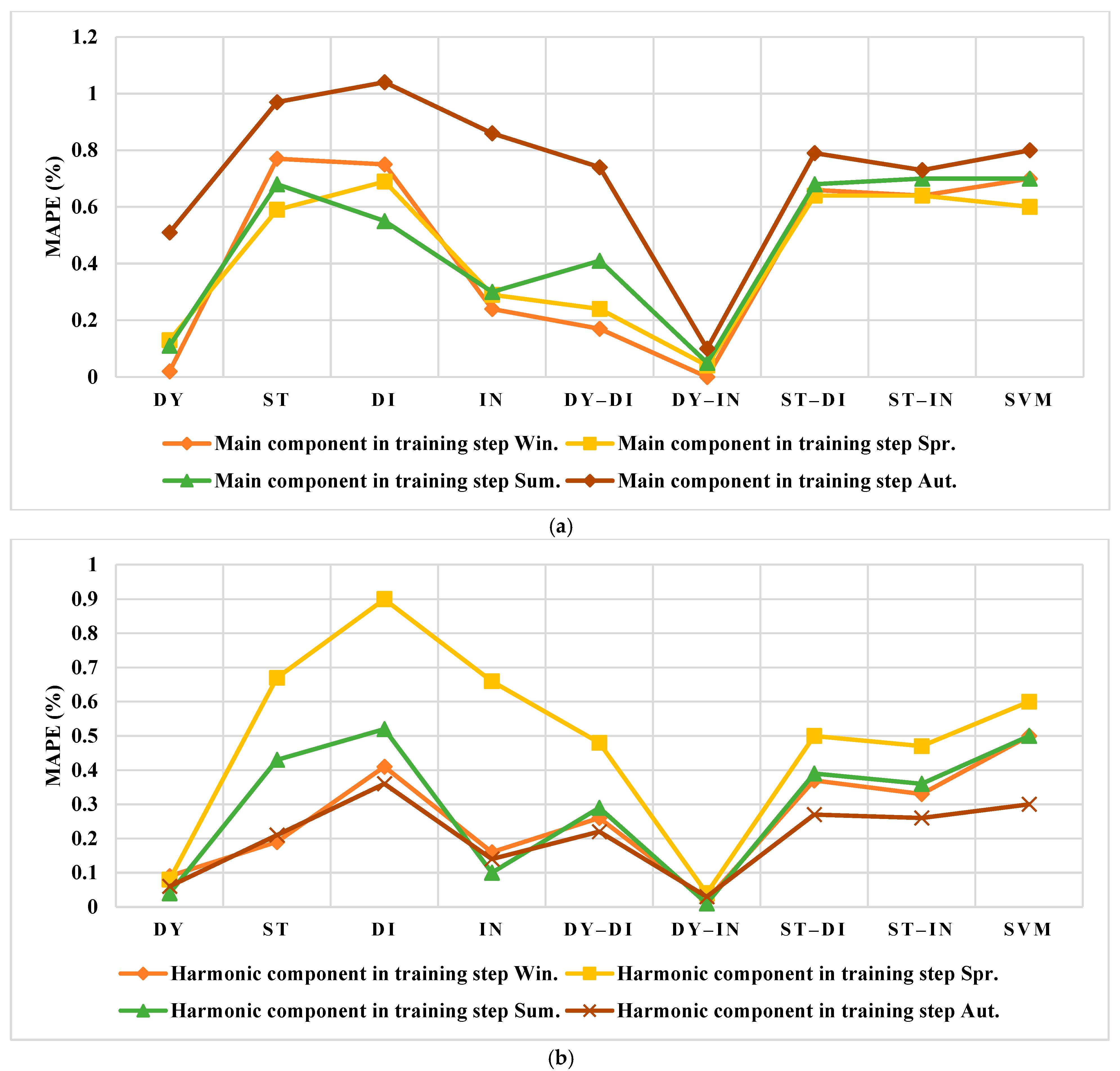
  • The results show that the best method is the dynamic indirect GP, which has the highest accuracy in comparison with the other methods. The proposed method is also compared to SVM and its accuracy is shown.

1.4. Paper Organization

The rest of the paper is organized as follows: in Section 2, the methodology of the paper is presented; Section 3 shows the results of EP forecasting in both the Spanish and the US electricity markets; in Section 4, the results are evaluated with metrics and the best model is appointed; and finally, Section 5 describes the conclusion.

2. Methodology

Electricity as a commodity has features that distinguish it from other commodities in terms of instantaneous price forecasting. Electricity supply and demand must always be in balance. Power generation and consumption take place at the same time and there is no storage capacity for this product in the network. These reasons allow price forecasting to be performed in three time horizons, which are the short term, medium term, and long term, and the medium-term forecast provides for the program. The planning of production units for repairs, water-heating units, and pumped water units, as well as long-term forecasting can have great impacts on the decision making for pre-purchase contracts and future contracts between buyers and sellers. In the meantime, price forecasting in the short term has the greatest impact on the pricing strategy compared to the medium- and long-term forecasts, so it has one of the most important advantages in the industry. The short-term forecast improves the bidding strategies of customers and sellers of electricity in the restructured electricity market. From the information available for accurate forecasting, the price is very important.
One of the most important advantages of short-term forecasting is the strategy for improving the supply and customers in the electricity market of the restructured power systems. Moreover, in a competitive market, the time series of EP consists of the high-frequency signal, mean, and variance values of the variable and multiple seasonal variations. Moreover, they are affected by the calendar, such as weekends and public holidays, high oscillations, and a high percentage of abnormal prices, mainly during periods with high demand [39]. These characteristics increase the complexity of EP forecasting. The EPs are inherently volatile, which makes market participation risky. In general, the factors affecting the EP can be classified as shown in Figure 1.

2.1. The Gaussian Processes Models

The GP is a well-known stochastic method that could be described as a set of time variables and space parameters. Additionally, the subset of the mentioned parameters is predefined as a mixture of multi-variation Gaussian distribution by two main functions, including the means function and covariance matrix. The calculations of ELM methods are often hard, and the variables should be forecasted [40]. To describe the performance of the GP, the following supposition is considered:
f ( x 1 ) f ( x 2 ) ( δ , Κ )
where x1 and x2 are the random variables, f is the estimated function, is the Gaussian distribution function, δ is mean function, and K is the CF. Additionally, shows the jointing operator, and indicates the supervision operator. If the number of random variables is more than two, the GP could cover them by using the matrix of CFs, as follows:
K ( x , x ) = [ k ( x 1 , x 1 ) k ( x 1 , x 2 ) k ( x 1 , x N ) k ( x i , x 1 ) k ( x i , x j ) k ( x i , x N ) k ( x N , x 1 ) k ( x N , x 2 ) k ( x N , x N ) ]
where N is the number of variables, K(x, x) is the matrix of CF that includes the set of correlational relations of any two variables of xi and xj, i.e., k(xi, xj), 1 ≤ i, jN. To learn the HPs in the GP that describe the CF behaviors, the following probability function should be maximized:
log p ( f | x , ) = 1 2 f T K 1 f 1 2 log | K | N 2 log ( 2 π )
where shows the HPs vector, and p is the multivariate Gaussian distribution as follows:
p ( f ( x ) ) = ( δ ( x ) , K ( x , x ) )
The descriptions of various models of the GP, i.e., dynamic, static, direct, and indirect, are rendered in [36].

2.2. GP for Time Series Modeling

The GP could be used for time series analysis with an autoregressive setting. When a new observation, such as x′, is added to the dataset of GP models, the CFs are redefined as follows:
K ( x , x ) = { k ( x , x 1 ) , k ( x , x 2 ) , , k ( x , x N ) }
In the time series, the set of x′ could be modified as the test data, i.e., x′ = xt. To complete the vector of prior observations (or test data), and considering P and i as the number of prior observations and time instances in the past, respectively, this vector could be proposed as xti = (yt–1–i, yt–2–i, yt–3–i, …, ytPi). Therefore, the train data should be described as x = (xt–1, xt–2, xt–3, …, xtN)T. The CFs matrix for the mentioned test and train data will be changed to the following:
{ K ( x , x ) = [ k ( x t 1 , x t 1 ) k ( x t 1 , x t N ) k ( x t 2 , x t 1 ) k ( x t 2 , x t N ) k ( x t N , x t 1 ) k ( x t N , x t N ) ] K ( x t , x ) = { k ( x t , x t 1 ) , k ( x t , x t 2 ) , , k ( x t , x t N ) }

2.3. The CFs for Time Series

There are various CFs used in previous studies. In this paper, we employed some main CFs to benchmark them: squared exponential (SE), Matérn 3 (M3), Matérn 5 (M5), and combinations of these main CFs as follows:
C F SE 1 ( r ) = σ f 2 exp ( r 2 2 2 )
C F M 3 2 ( r ) = σ f 2 ( 1 + 3 r ) exp ( 3 r )
C F M 5 3 ( r ) = σ f 2 ( 1 + 3 r + 5 r 2 3 2 ) exp ( 5 r )
C F SE M 3 4 ( r ) = σ f 2 ( 1 + 3 r ) exp ( 3 r 3 2 3 )
C F SE + M 3 5 ( r ) = σ f 2 { exp ( r 2 2 2 ) + ( 1 + 3 r ) exp ( 3 r ) }
C F SE + M 5 6 ( r ) = σ f 2 { exp ( r 2 2 2 ) + ( 1 + 3 r + 5 r 2 3 2 ) exp ( 5 r ) }
where σ f 2 > 0 is the signal variance and > 0 is the length scale of the HPs. Moreover, r is desired as follows:
r = x x
The flowchart of the proposed method is presented in Figure 2.

3. Results

3.1. Performance Metrics

For evaluation of the proposed models, their results should be benchmarked with ability and errors in prediction as follows:
M A P E = 1 T t = 1 T | y ^ t y t y t |
N R M S E = 1 T t = 1 T ( y ^ t y t max ( y ) min ( y ) ) 2
P I C P = 1 T t = 1 T ξ t , ξ t = { 1 L t y t U t 0 o t h e r w i s e
P I N A W = 1 W T t = 1 T ( U t L t )
I S = 1 T t = 1 T y ^ t min ( y ) max ( y ) min ( y )
T I C = ( 1 T t = 1 T ( y ^ t y t ) 2 ) / ( 1 T t = 1 T ( y ^ t ) 2 + 1 T t = 1 T ( y t ) 2 )
A C E = P I C P P I N C
In this paper, to evaluate the prediction accuracy, five metrics are used: the mean absolute percentage error (MAPE), normalized root mean square error (NRMSE), prediction interval coverage probability (PICP), interval sharpness (IS), and prediction interval normalized average width (PINAW). Moreover, Theil’s inequality coefficient (TIC) and average coverage error (ACE) are employed to measure the method’s ability for prediction. It provides a measure of how well a time series of estimated values compares to a corresponding time series of observed values. In (14)–(20), T is the length of the time series, y ^ t is the forecasted value, yt is the actual value, and y is the time series value. Additionally, Lt and Ut are the lower and upper bands of the prediction interval (PI), and PINC is considered as the PI nominal confidence with a variation between 10 and 90%. In this paper, the value of PINC is considered to be 80%. Finally, in (19), the value of W is the PI average width, which indicates the maximum and minimum difference between the observed value.

3.2. Data

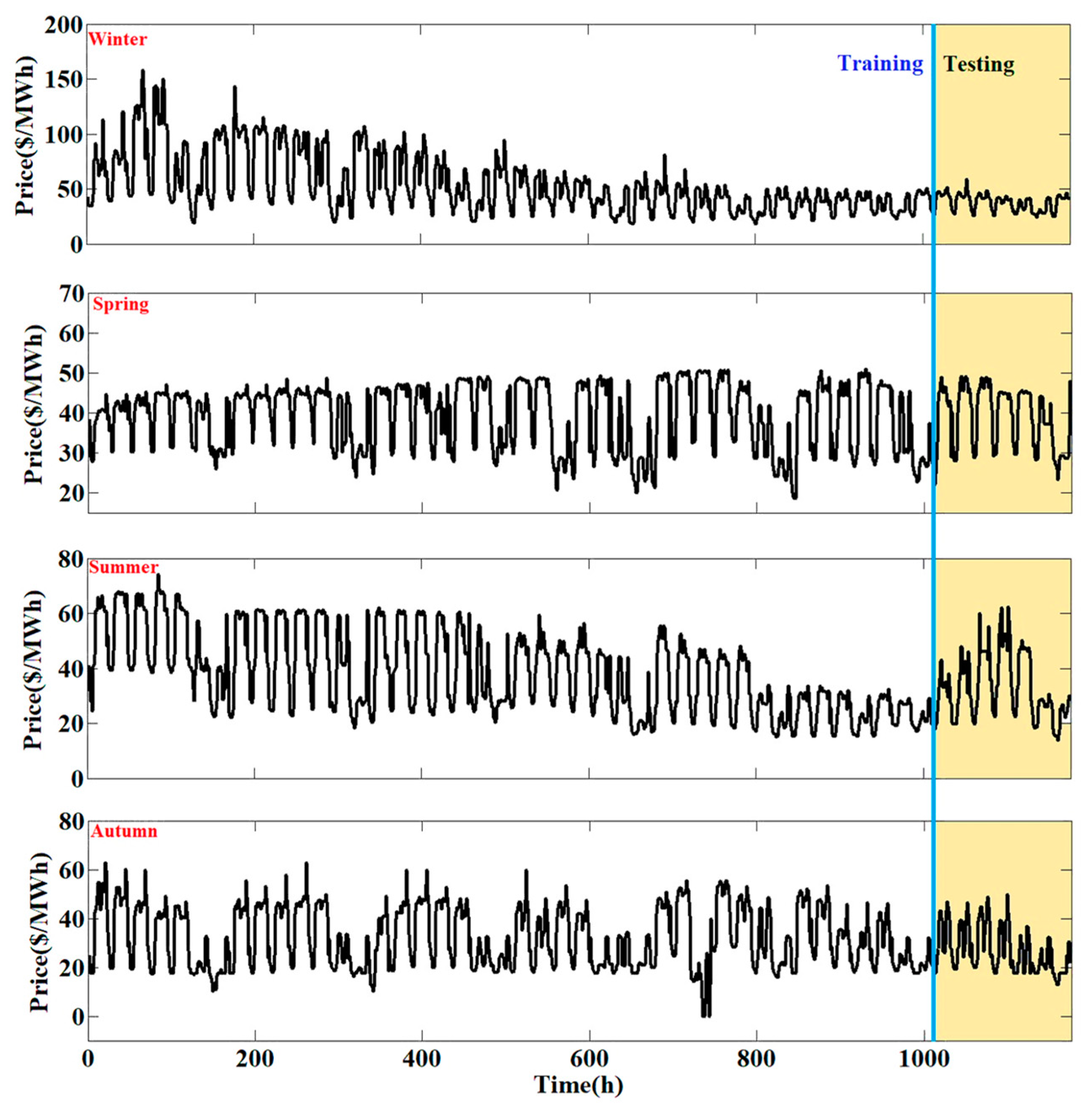
3.2.1. The Spanish Electricity Market

The Spanish electricity market is one of the largest physical markets in the world, providing daily market services to market participants. The data used in this paper are quarterly and related to 2019 [27]. The required data for the interval are given in Table 1. Moreover, the time series of EP in all seasons are presented in Figure 3 [41]. As seen in Figure 3, the electricity market of Spain fluctuates sharply and includes variable variance.

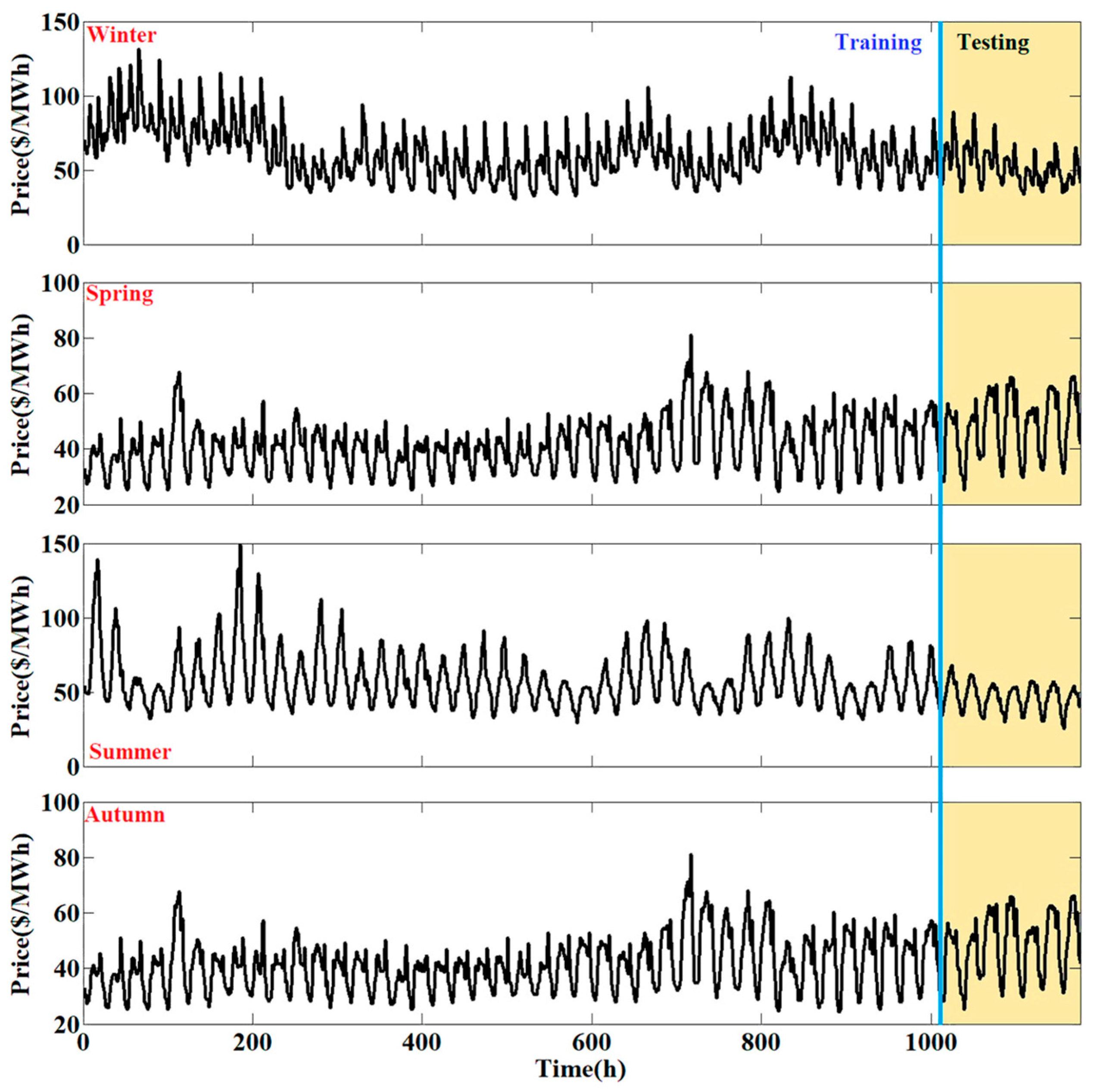
3.2.2. The US Electricity Market

The training and testing data of the electricity market of the US for 2018 are given in Table 2. Moreover, the hourly ahead data for the considered data of all seasons are shown in Figure 4 [42]. As seen in Figure 4, the variation in EPs for the electricity market of the US is less than that in Spain.

3.2.3. Data Analysis

By examining Figure 3 and Figure 4, the following results can be seen:
  • The EP decreases at the beginning of the day and increases at night;
  • On different days of each week, the EP is different and declines towards the weekend;
  • The price in the early hours of midnight on weekdays is low. As daylight approaches, the EP increases, and in the middle of the day it reaches the maximum value. Therefore, it will be more useful if the main power system is divided into several subsystems to enhance the model’s performance;
  • The EP on holidays is lower than on weekdays, due to lower consumption from large industrial factories.
In order to obtain a high accuracy of results, the multi-step GP is used. In this method, the time series shown in Figure 3 and Figure 4 is decomposed into one main component and three harmonic components. The advantage of this decomposition is that the detail of EP could be achieved at any moment.

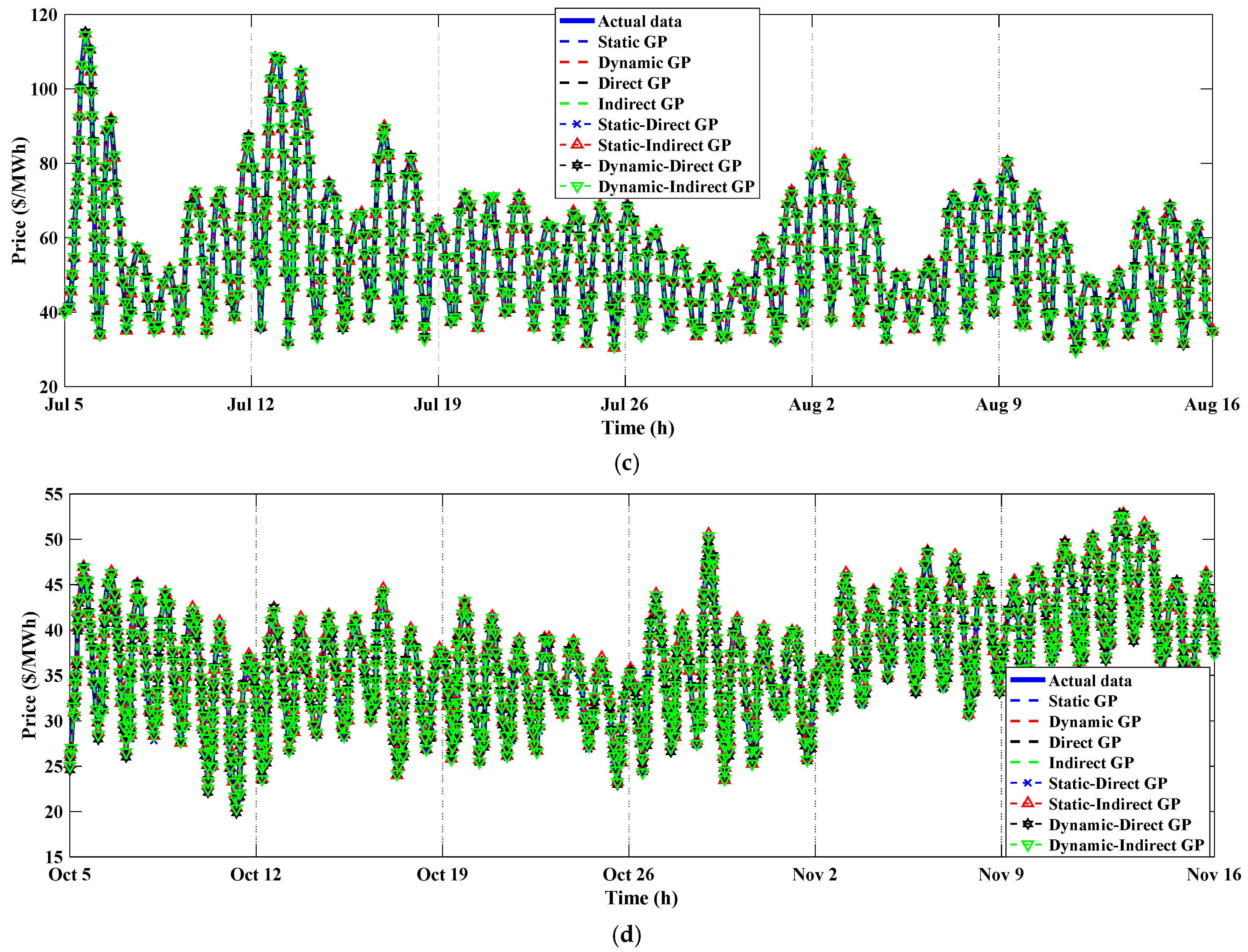
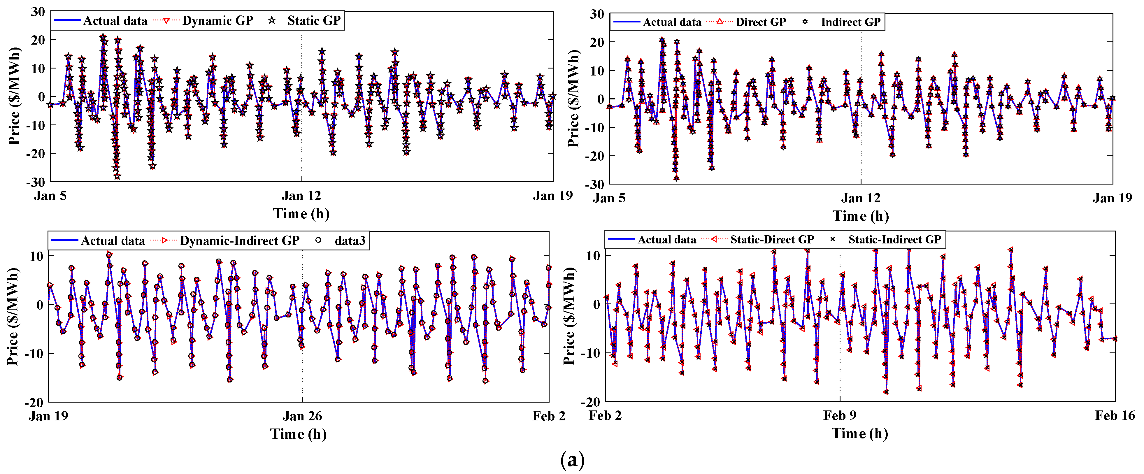
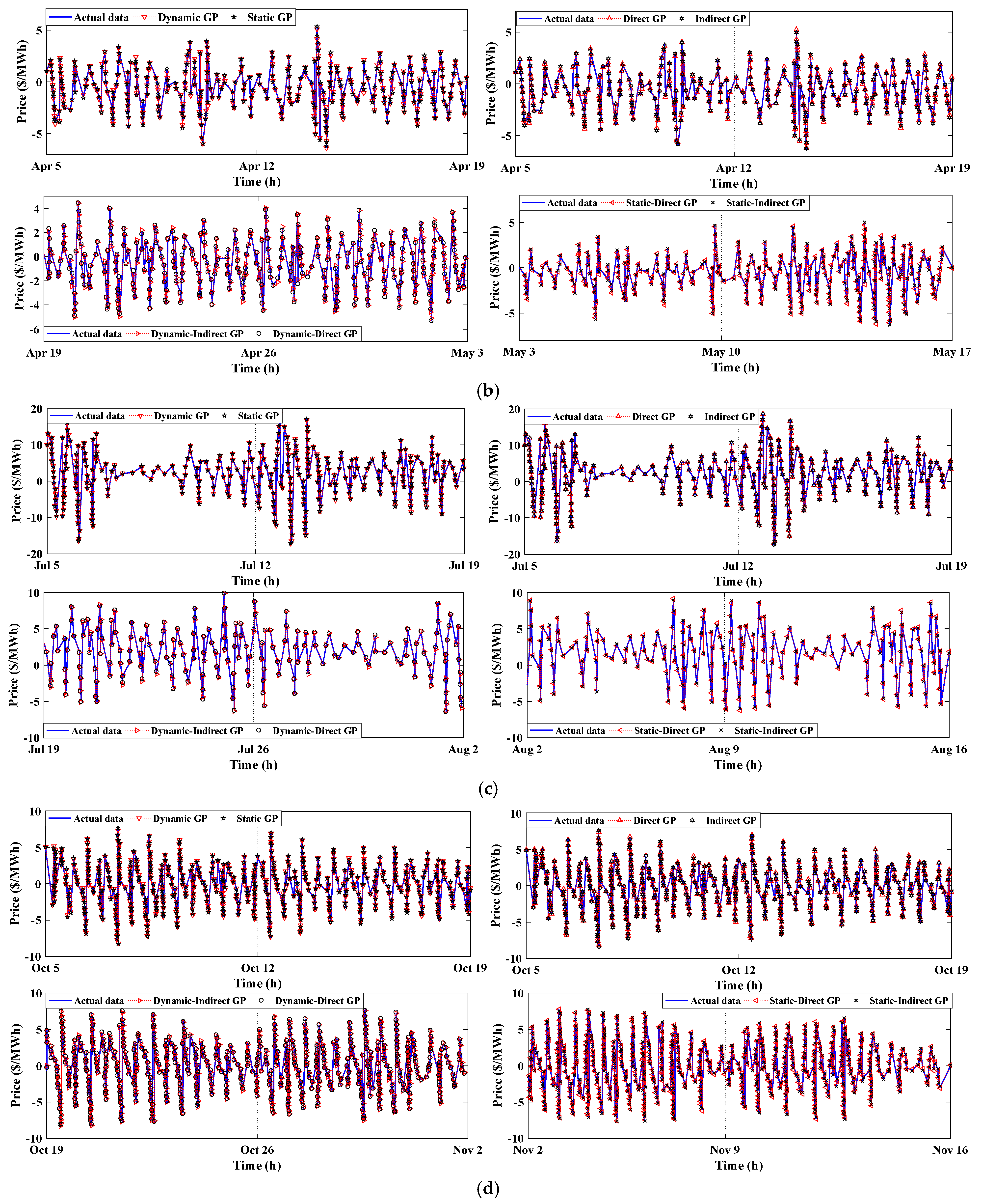
3.3. The Forecasting of the Training Data

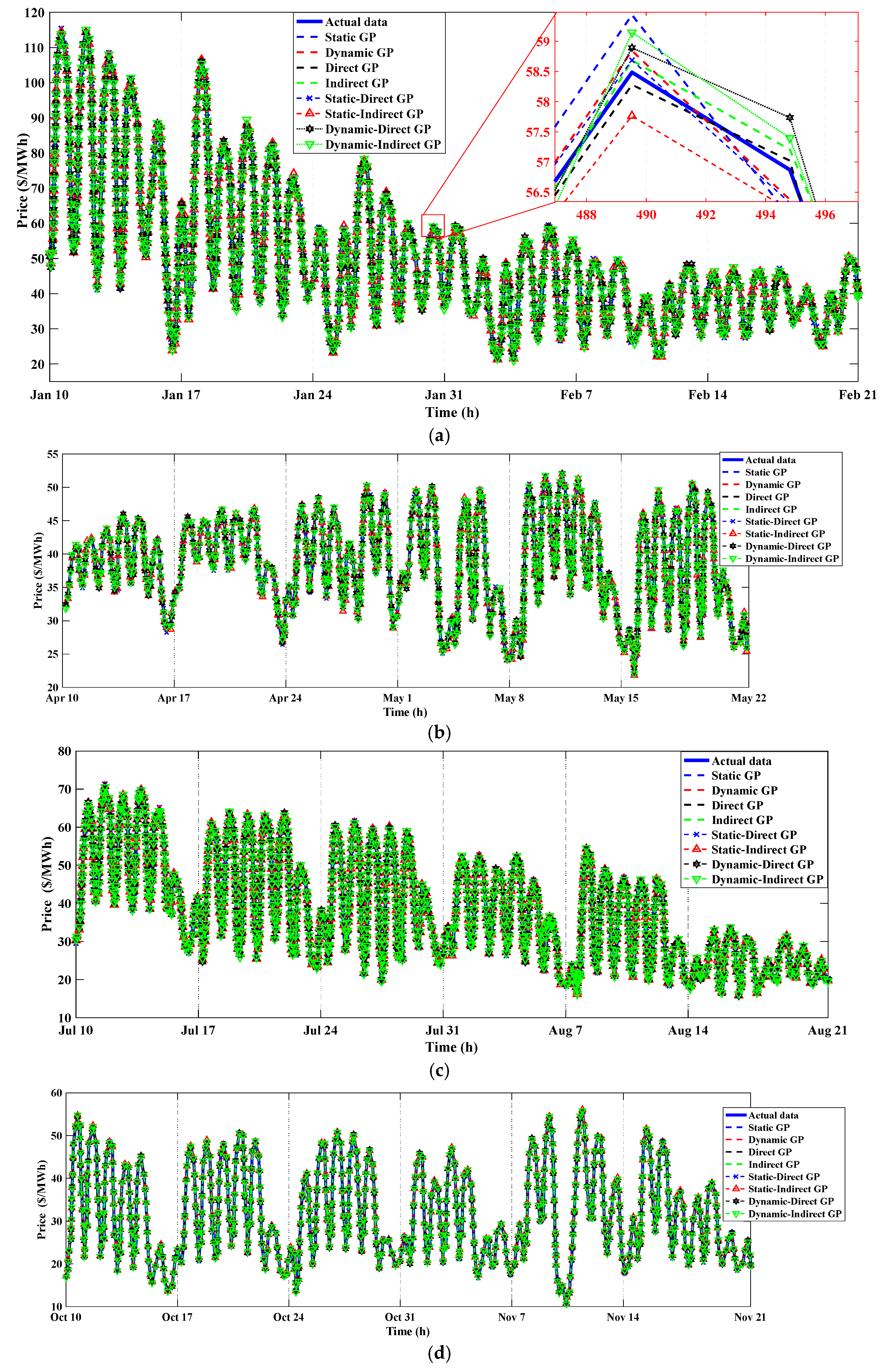
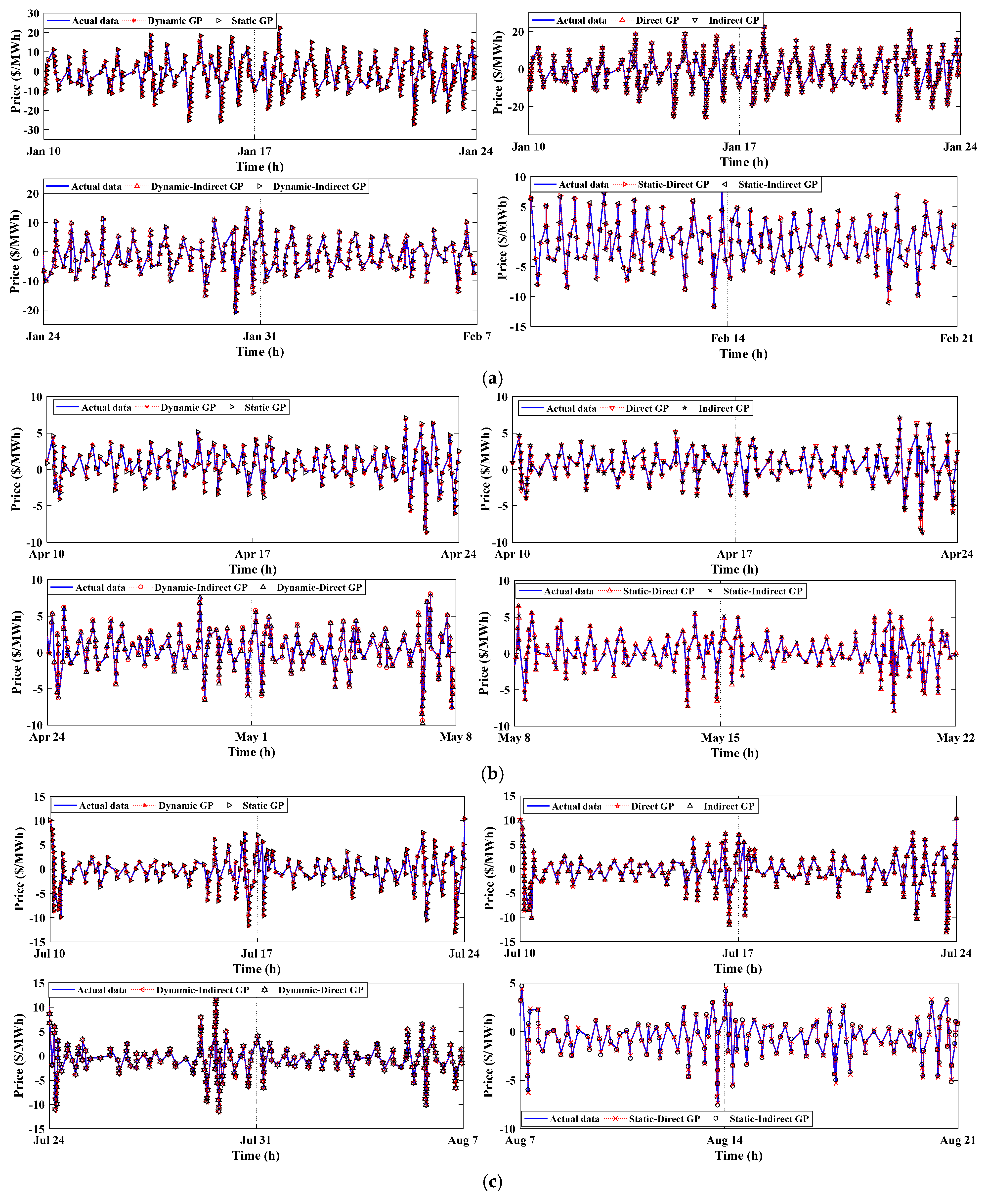
3.3.1. The Spanish Electricity Market

The first evaluation of the proposed methods is the forecasting of the training data. As mentioned before, the data of EPs will be divided into main and harmonic components. The forecasting of EPs in the training step for the main component is shown in Figure 5. In this figure, all seasons are presented, and the various models of the GP are tested. As shown in Figure 5a–d, the predicted results of all models are acceptable.
Figure 6 shows the prediction results of the sum of harmonic components of train data using all proposed models. In order to indicate clear results, each plot consists of four subplots that show the results of two weeks. Similar to the main components, the results of the harmonic components have high accuracies, as seen in Figure 6a–d. Moreover, the detailed evaluations are rendered in Section 4.

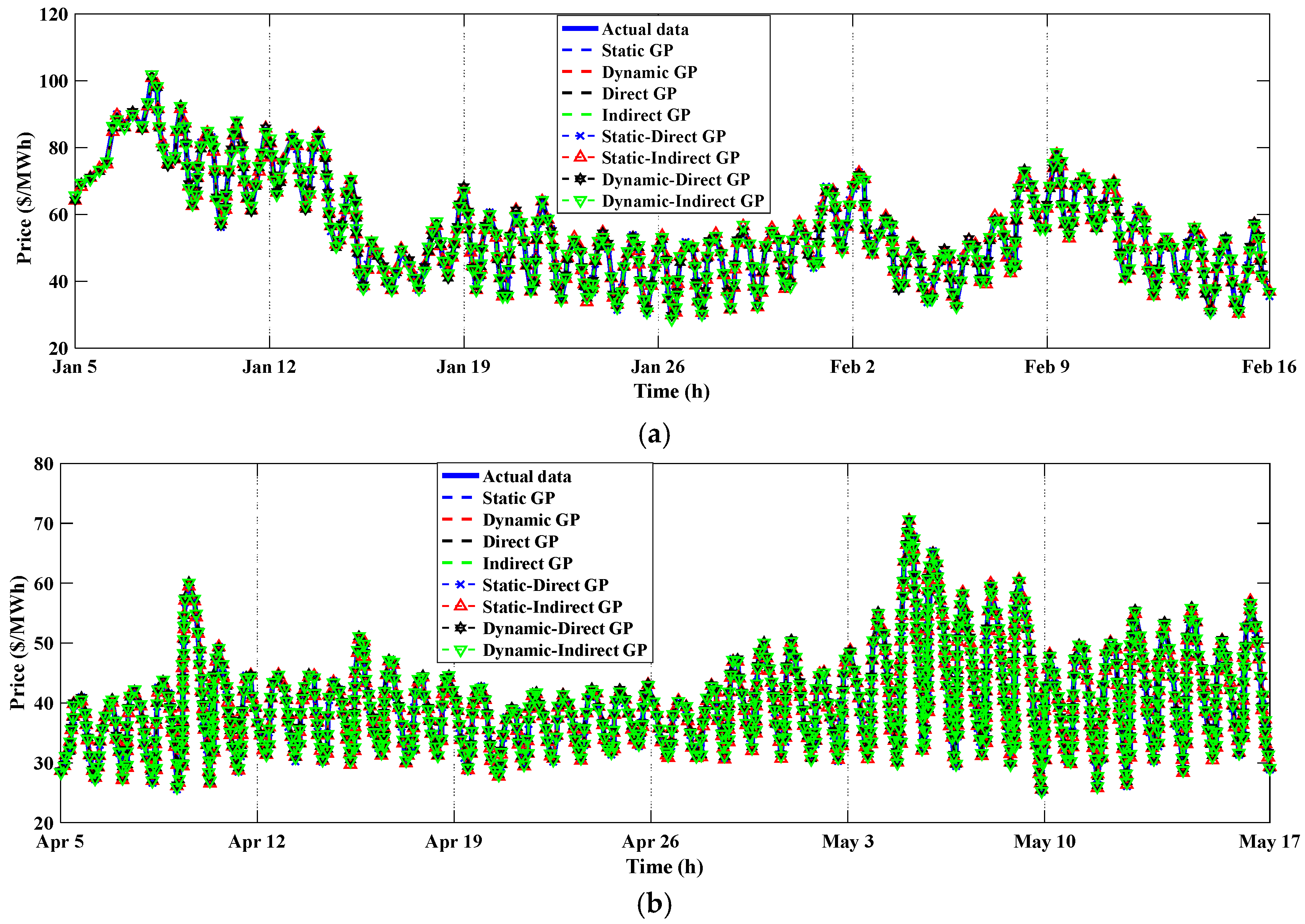
3.3.2. The US Electricity Market

The predicted values of the main components of EP for the US electricity market using all models are plotted in Figure 7. Moreover, the forecasting results of the sum of harmonic components are shown in Figure 8. The subplots of Figure 8a–d include two weeks. The results of all methods are approximately closed. The complete investigations of Figure 7 and Figure 8 are presented in Section 4 and are evaluated by the metrics of Table 1.

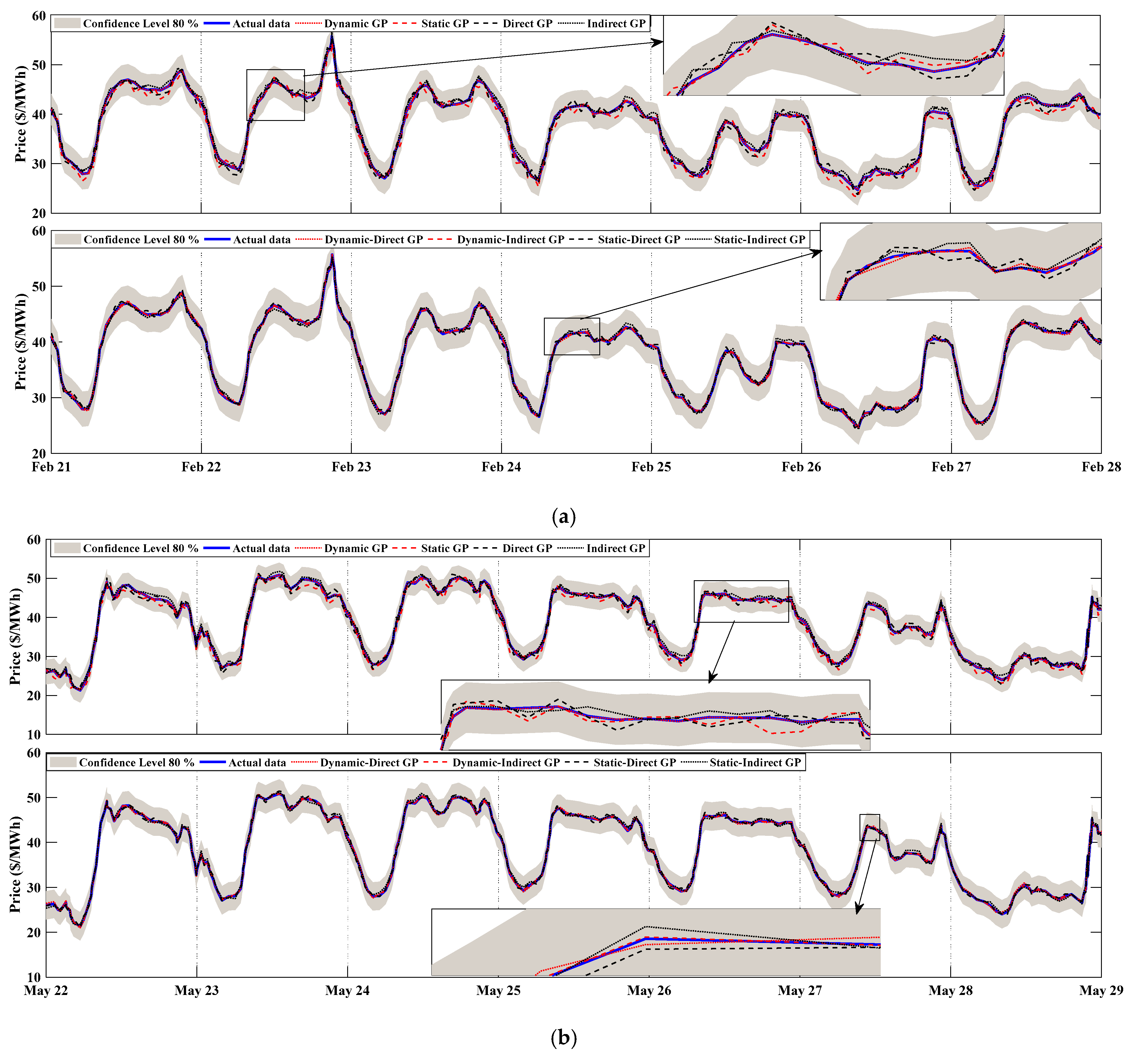
3.4. The Forecasting of the Testing Data

In this step, the test data of both US and Spain are forecasted. Based on the decomposition of the curves into main and harmonic components, the forecasting of these components is carried out. Finally, these components are composed, and the initial curves are obtained. All of these mentioned steps are followed for both the actual and predicted data in all seasons.

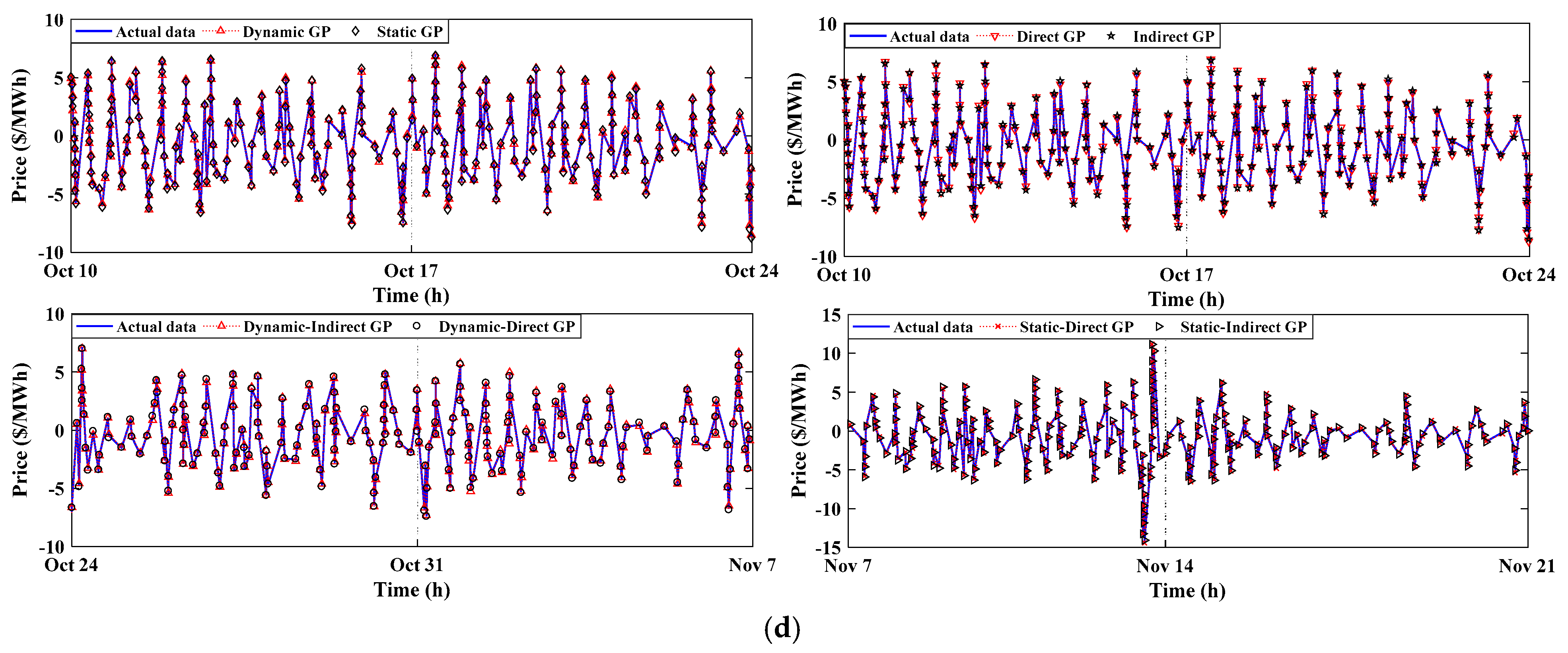
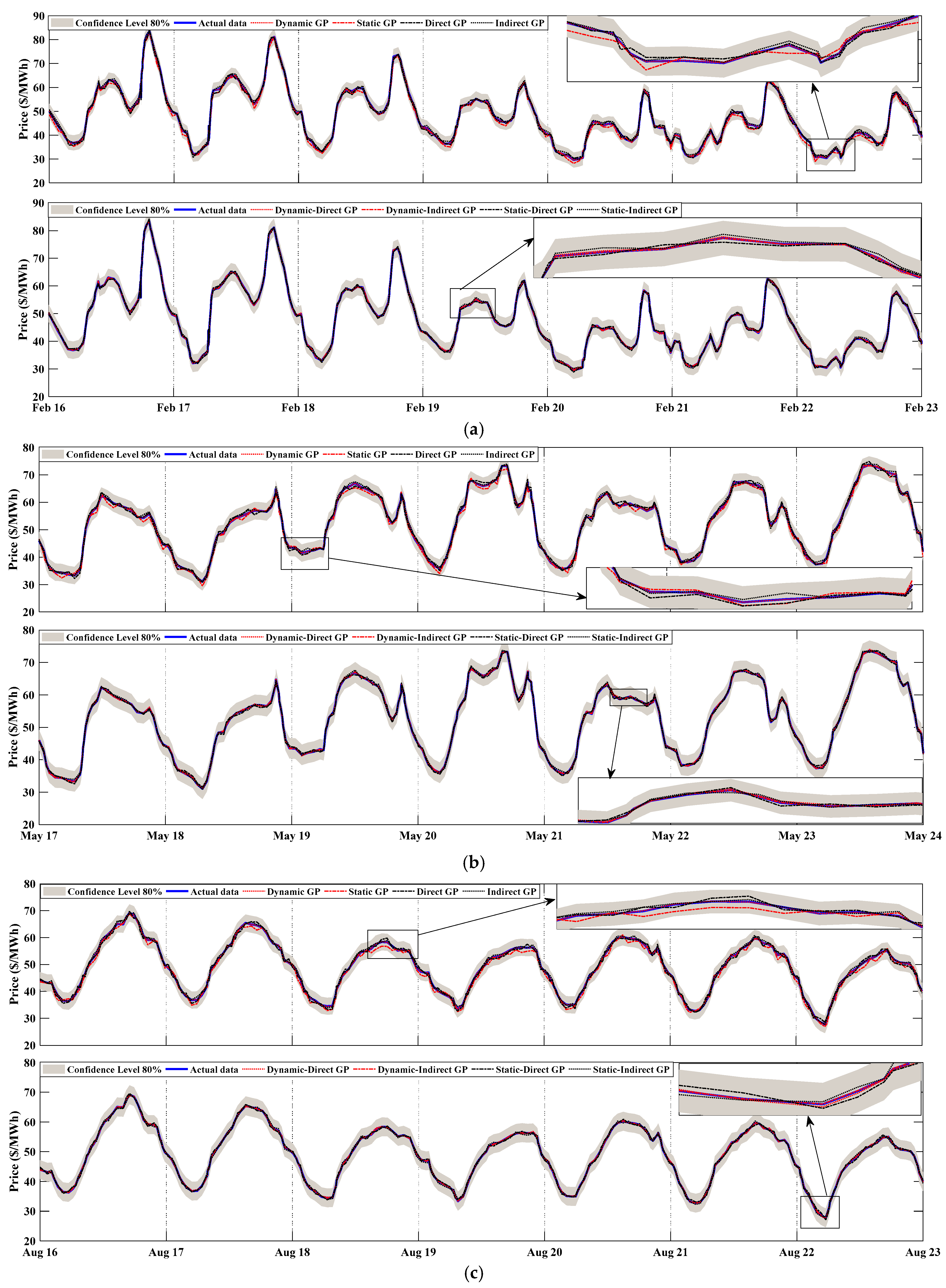
3.4.1. The Spanish Electricity Market

The forecasted results for all seasons of Spain, using various models, are carried out and presented in Figure 9a–d. As shown in all figures, the best forecaster method is the combination of the dynamic and indirect GP. Additionally, the dynamic GP is better than other individual models.

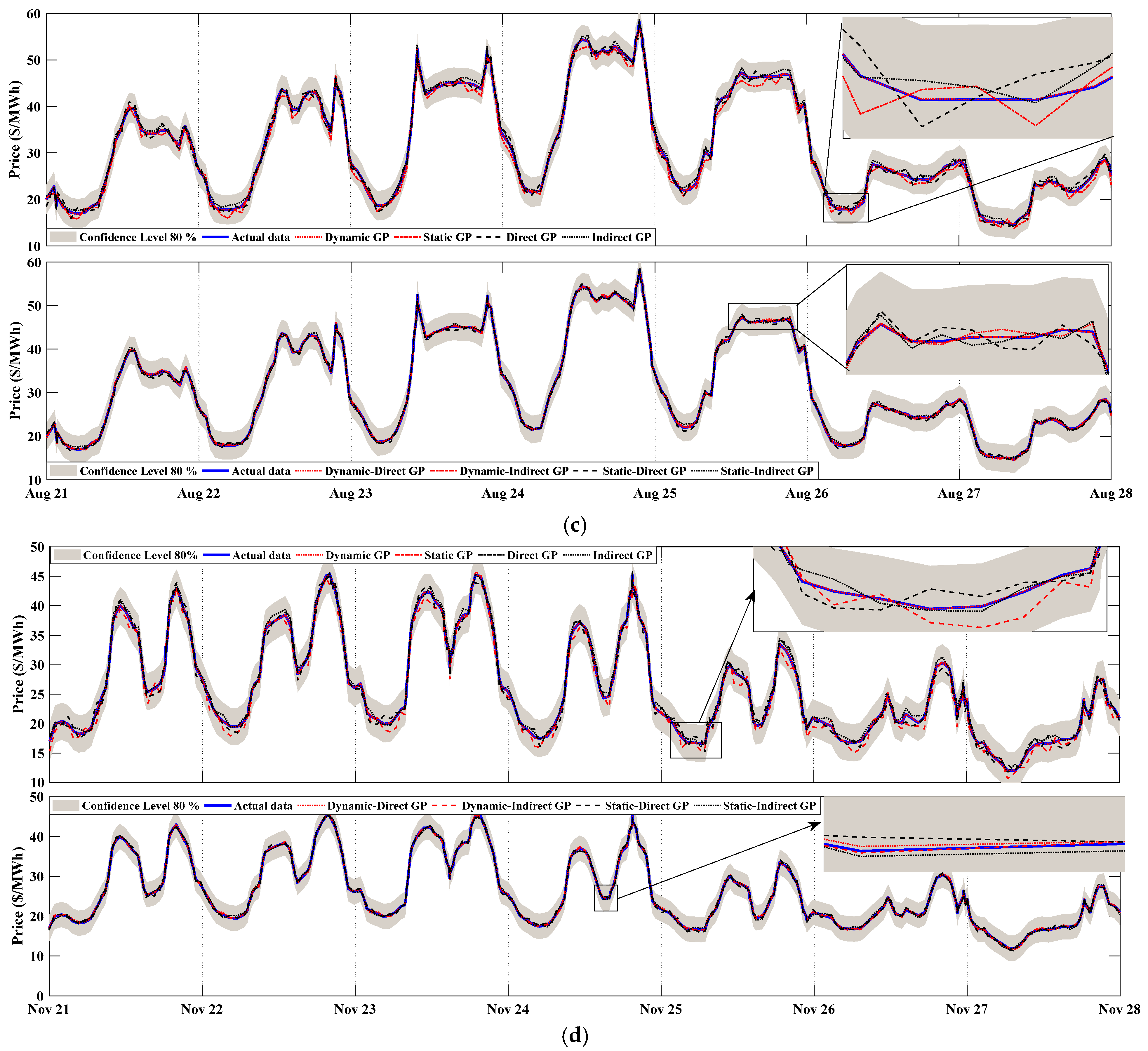
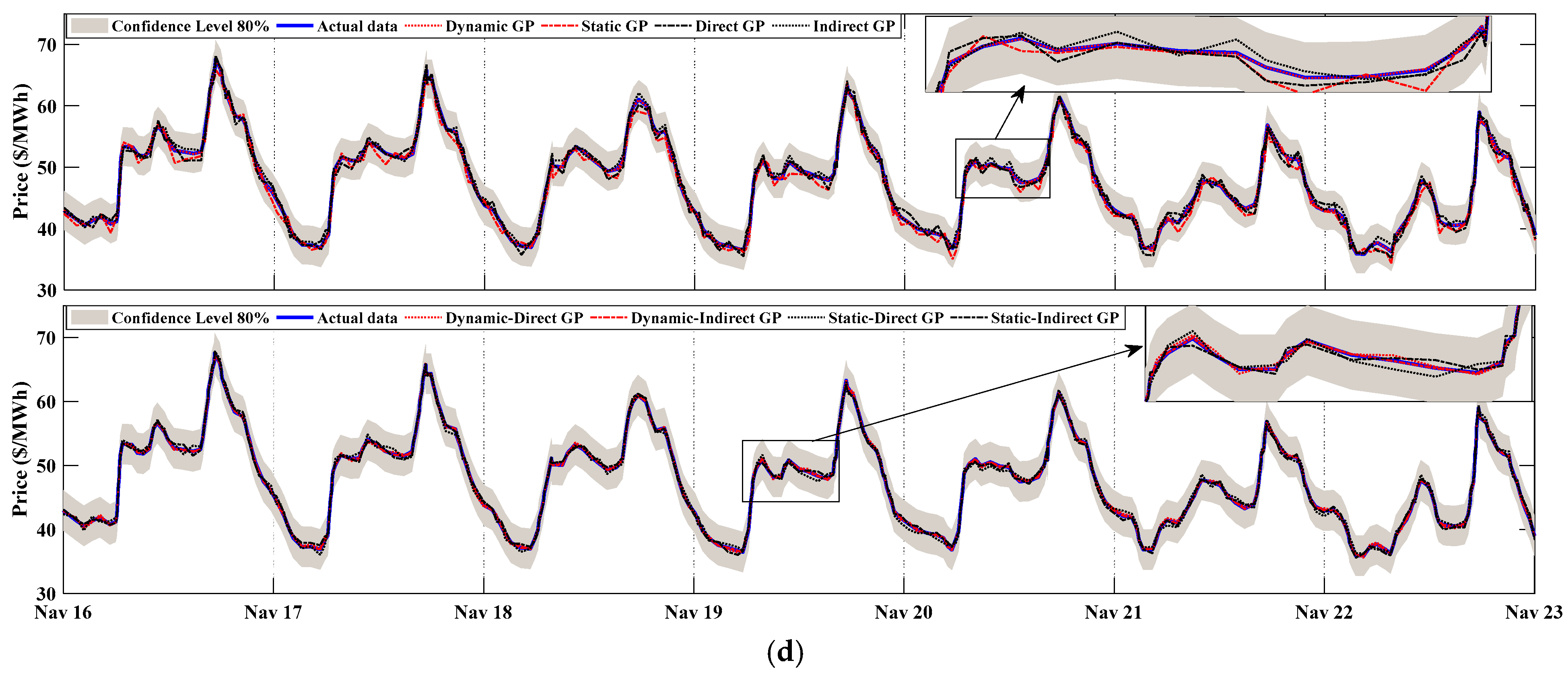
3.4.2. The US Electricity Market

The predicted results for all seasons of the US are shown in Figure 10a–d. As shown in these figures, the dynamic indirect GP is better than other combination methods. Further evaluation of the results is presented in the next section.

4. Discussion

The time series related to EPs in different seasons has decomposed into harmonic components. The main component has a non-linear instinct; however, the harmonic components are linear.
By analyzing the time series of the main component of EP in the winter of Spain (see Figure 5a), it can be seen that the EP at the beginning of the season has higher price fluctuations compared to the last days of the season. Additionally, the harmonic component has more fluctuations and amplitudes at the beginning of the season (see Figure 6a). By analyzing the time series of the main component of EP in the summer of Spain, according to Figure 5c, this component has uniform fluctuations and amplitudes, which is also seen in the harmonic component (see Figure 6c). With analyzing the time series of all components of the EP in the spring of Spain, there are several non-uniform fluctuations with a large amplitudes, as shown in Figure 5b and Figure 6b. This problem is also cleared in autumn; its time series are plotted in Figure 5d and Figure 6d.
The time series of both the main and harmonic components of EPs in winter in the US show that it has a linear behavior and has uniform fluctuations and amplitude during the season. This claim could be found in Figure 7a and Figure 8a, and also it could be expanded to summer and autumn, based on Figure 7c,d and Figure 8c,d. Finally, using a simple analysis of the time series of the main and harmonic components of EPs in spring of the US, according to Figure 7b and Figure 8b, there are several fluctuations and non-uniform amplitudes in the time series. The results of the evaluation metrics of all methods for all presented data are shown in the following figures for both Spain and the US. Additionally, in these figures, the abbreviations of Win., Spr., Sum., and Aut. indicate the winter, the spring, the summer, and the autumn, respectively. In addition, the abbreviations of DY, ST, DI, and IN indicate the dynamic, static, direct, and indirect, respectively.

4.1. Results Evaluation of Spain

As seen in Figure 11, the value of MAPE for all models in the training data is close to zero, which shows a high ability to make predictions. However, the robust method in the training step is related to the dynamic indirect GP in the main component of winter, which is 0.00%. This means that all obtained data by this method equal actual data. Moreover, the dynamic GP is better than the other individual models, i.e., static, direct, and indirect. For instance, the MAPE in the summer of the test step with the dynamic GP is obtained as 2.15%, which is lower by about 5.5% than the static and the direct GP, and about 2.2% lower than the indirect GP. The results show that with a combination of the two robust individual models, the results are better than those from these individual models. The dynamic and indirect GP models are better than the static and direct models, and the results of all evaluated data are better than both the dynamic and indirect models. In addition, the proposed method is better than SVM. The results of SVM could be compared with ST–DI, ST–IN, and DI.
The results of NRMSE are presented in Figure 12. In this figure, the lowest values are related to the dynamic indirect GP. Other methods are weak in comparison with this method. Additionally, the best result obtained by the dynamic indirect GP in the test data is related to the winter with 0.43%. In addition, the NRMSE results of SVM are much higher than those of DY–IN, and are close to the DI and ST models.
The value of PICP should be higher than the PI confidence, which is considered 80%. The obtained values for this metric in Figure 13 show the robustness of the GP. Moreover, the PICP of the dynamic indirect GP is higher than that in other models, especially in test analysis. All the values of PICP with the DY–IN are much higher than those of SVM.
The minimum values of PINAW are the best results that are shown in Figure 14. Similar to the other previous metrics, the best results are reached in the dynamic indirect GP, and its highest PINAW is related to the autumn test data, i.e., 9.28%. However, it is lower than the other models by at least 2%. It should be noted that the closest model to this model in Figure 14 is the dynamic GP. As seen in Figure 14, the results obtained by SVM could be placed between the results of ST and DI. However, the other models of GP are better than SVM.
Based on (18), the results of average IS for Spain are shown in Figure 15. Based on this figure, the highest values are cleared in the dynamic indirect GP model. Moreover, the lowest value is −8.55, related to the static GP in the autumn of the test step, while the corresponding value for the dynamic indirect GP is −0.95. In addition, by comparing the results of DY–IN and SVM in Figure 15, it can be found that the proposed method is better than SVM.
Finally, TIC shows the prediction ability of the method. This metric should be low to indicate the advantage of the method. In the individual models, the dynamic GP and the direct GP are the best and the worst methods, respectively, as shown in Figure 16. Additionally, in the combination models, the best results are obtained by the dynamic indirect GP, and the highest values have resulted in the cases with the static GP, i.e., the static direct GP and the static indirect GP.

4.2. Results Evaluation of the US

The evaluation of results for the US is summarized in Figure 17, Figure 18, Figure 19, Figure 20, Figure 21 and Figure 22. As shown in these figures, the best method is chosen as the dynamic indirect GP because of its low error rate and high prediction ability. Additionally, the result for the US is a little better than that of Spain due to normal and uniform time series. The maximum error in MAPE in the test data of the dynamic indirect GP is accrued in winter and autumn, which is better than the static GP (2% in comparison with 10%). The RMSE for the US has a similar discussion to MAPE. In addition, the results of SVM are close to those of the DI model.
The best prediction accuracy with higher than 97% and a maximum of 99.99% is related to the dynamic indirect GP that is shown in Figure 19. However, other combination methods have similar results. Additionally, the dynamic GP could realize 95% prediction of test data on average.
It is clear in Figure 20 that the only the dynamic indirect GP could decrease the PINAW in the test data prediction after the training step. The PINAW value of the test data by other models is almost variated from the values of training data.
The values of IS by the dynamic indirect GP are closer to zero in comparison to the other methods, especially in the test step results of the static GP, indirect GP, and direct GP. Therefore, based on the information in Figure 21, the best manner is the dynamic indirect GP.
Finally, Figure 22 shows the values of TIC. In this figure, the lowest results, which are close to zero, only appear in the dynamic indirect GP results. For example, the TIC values for the spring of the test step are 0.49 and 0.25 related to the static direct GP and the dynamic GP, respectively; however, they are higher than 0.07, which is the value obtained by the dynamic indirect GP. Other examples can be found in all seasons when the ability of the dynamic indirect GP is higher than other methods, especially individual models.

5. Conclusions

In this paper, firstly, various models of GP as dynamic, static, direct, and indirect are considered, and their combinations are proposed to forecast the EP of two electricity markets in the US and Spain. The GP is a robust stochastic method that could be reformed into time series problems. In this paper, six CFs are used to validate the training and testing data. In addition, the time series of both the training data and the testing data are decomposed into the main and harmonics components, and the multi-prediction is applied in this paper to increase the accuracy. The results obtained by different methods are evaluated using various metrics and the best method is introduced as the dynamic indirect GP. Its error is close to zero, which shows the robustness of the proposed model. Moreover, the results show that the accuracy of combination models of GP is better than the individual models by at least 1–5%. Moreover, the dynamic GP is better than other the individual models. Moreover, the results of SVM are also rendered and have similar results to the direct GP. The forecasting results show that if the time series of EP is uniform, a better accuracy will be obtained. This issue is supported by a comparison of the two different electricity markets. The results of the test step showed that the best of all methods is the dynamic indirect GP, which obtained the highest PICP (about 99% for both the US and Spain markets), and the lowest PINAW (about 9% for both the USA and Spain markets). In addition, in all results, the static GP is known to be the worst method, due to having the lowest PICP (about 90% for both the USA and Spain markets) and the highest PINAW (about 17% for both the USA and Spain markets).

Author Contributions

Conceptualization: A.D.; methodology: A.A.; software, A.A.; validation, A.D. and A.A.; formal analysis, A.D.; investigation, A.D.; resources, A.A.; data curation, A.A.; writing—original draft preparation, A.D. and A.A.; writing—review and editing, A.D.; visualization, A.A.; supervision, A.D.; project administration, A.D. All authors have read and agreed to the published version of the manuscript.

Funding

This research received no external funding.

Institutional Review Board Statement

Not applicable.

Informed Consent Statement

Not applicable.

Data Availability Statement

Not applicable.

Conflicts of Interest

The authors declare no conflict of interest.

References

  1. Yang, W.; Wang, J.; Niu, T.; Du, P. A novel system for multi-step electricity price forecasting for electricity market management. Appl. Soft Comput. 2019, 88, 106029. [Google Scholar] [CrossRef]
  2. Seyed Shenava, S.J.; Dejamkhooy, A.; JavanAjdadi, K. Short-term Electric Load Forecasting Using Grey Models by Considering Demand Response. Comput. Intell. Electr. Eng. 2018, 8, 1–16. [Google Scholar]
  3. Ahmadpour, A.; Mokaramian, E.; Anderson, S. The effects of the renewable energies penetration on the surplus welfare under energy policy. Renew. Energy 2020, 164, 1171–1182. [Google Scholar] [CrossRef]
  4. Huang, C.J.; Shen, Y.; Chen, Y.H.; Chen, H.C. A novel hybrid deep neural network model for short-term electricity price forecasting. Int. J. Energy Res. 2021, 45, 2511–2532. [Google Scholar] [CrossRef]
  5. Amjady, N.; Daraeepour, A. Design of input vector for day-ahead price forecasting of electricity markets. Expert Syst. Appl. 2009, 36, 12281–12294. [Google Scholar] [CrossRef]
  6. Deng, Z.; Liu, C.; Zhu, Z. Inter-hours rolling scheduling of behind-the-meter storage operating systems using electricity price forecasting based on deep convolutional neural network. Int. J. Electr. Power Energy Syst. 2020, 125, 106499. [Google Scholar] [CrossRef]
  7. Golmohamadi, H.; Larsen, K.G.; Jensen, P.G.; Hasrat, I.R. Optimization of power-to-heat flexibility for residential buildings in response to day-ahead electricity price. Energy Build. 2021, 232, 110665. [Google Scholar] [CrossRef]
  8. Nowotarski, J.; Weron, R. Recent advances in electricity price forecasting: A review of probabilistic forecasting. Renew. Sustain. Energy Rev. 2018, 81, 1548–1568. [Google Scholar] [CrossRef]
  9. Wang, J.; Yang, W.; Du, P.; Niu, T. Outlier-robust hybrid electricity price forecasting model for electricity market management. J. Clean. Prod. 2020, 249, 119318. [Google Scholar] [CrossRef]
  10. Zhao, Z.; Wang, C.; Nokleby, M.; Miller, C.J. Improving short-term electricity price forecasting using day-ahead LMP with ARIMA models. In 2017 IEEE Power & Energy Society General Meeting; IEEE: New York, NY, USA, 2017; pp. 1–5. [Google Scholar]
  11. Kumar, V.; Singh, N.; Singh, D.K.; Mohanty, S.R. Short-Term Electricity Price Forecasting Using Hybrid SARIMA and GJR-GARCH Model. In Networking Communication and Data Knowledge Engineering; Springer: Singapore, 2017; pp. 299–310. [Google Scholar]
  12. Marín, J.B.; Orozco, E.T.; Velilla, E. Forecasting electricity price in Colombia: A comparison between neural network, ARMA process and hybrid models. Int. J. Energy Econ. Policy 2018, 8, 97. [Google Scholar]
  13. Brusaferri, A.; Matteucci, M.; Portolani, P.; Vitali, A. Bayesian deep learning based method for probabilistic forecast of day-ahead electricity prices. Appl. Energy 2019, 250, 1158–1175. [Google Scholar] [CrossRef]
  14. Kavaklioglu, K. Principal components based robust vector autoregression prediction of Turkey’s electricity consumption. Energy Syst. 2019, 10, 889–910. [Google Scholar] [CrossRef]
  15. Korir, E.K.; Aduda, J.; Mageto, T. Forecasting Electricity Prices Using Ensemble Kalman Filter. J. Stat. Econometr. Methods 2020, 9, 27–45. [Google Scholar]
  16. Singh, S.; Hussain, S.; Bazaz, M.A. Short term load forecasting using artificial neural network. In 2017 Fourth International Conference on Image Information Processing (ICIIP); IEEE: Piscataway, NJ, USA; pp. 1–5.
  17. Alshejari, A.; Kodogiannis, V.S. Electricity price forecasting using asymmetric fuzzy neural network systems. In 2017 IEEE International Conference on Fuzzy Systems (FUZZ-IEEE); IEEE: Piscataway, NJ, USA, 2017; pp. 1–6. [Google Scholar]
  18. Ugurlu, U.; Oksuz, I.; Tas, O. Electricity Price Forecasting Using Recurrent Neural Networks. Energies 2018, 11, 1255. [Google Scholar] [CrossRef] [Green Version]
  19. Marcjasz, G.; Lago, J.; Weron, R. Neural networks in day-ahead electricity price forecasting: Single vs. multiple outputs. multiple outputs. arXiv 2020, preprint. [Google Scholar] [CrossRef]
  20. Heydari, A.; Nezhad, M.M.; Pirshayan, E.; Garcia, D.A.; Keynia, F.; De Santoli, L. Short-term electricity price and load forecasting in isolated power grids based on composite neural network and gravitational search optimization algorithm. Appl. Energy 2020, 277, 115503. [Google Scholar] [CrossRef]
  21. Bisoi, R.; Dash, P.K.; Das, P.P. Short-term electricity price forecasting and classification in smart grids using optimized multikernel extreme learning machine. Neural Comput. Appl. 2018, 32, 1457–1480. [Google Scholar] [CrossRef]
  22. Yan, X.; Chowdhury, N.A. Mid-term electricity market clearing price forecasting: A multiple SVM approach. Int. J. Electr. Power Energy Syst. 2014, 58, 206–214. [Google Scholar] [CrossRef]
  23. Kuo, P.-H.; Huang, C.-J. An Electricity Price Forecasting Model by Hybrid Structured Deep Neural Networks. Sustainability 2018, 10, 1280. [Google Scholar] [CrossRef] [Green Version]
  24. Wang, K.; Xu, C.; Zhang, Y.; Guo, S.; Zomaya, A.Y. Robust Big Data Analytics for Electricity Price Forecasting in the Smart Grid. IEEE Trans. Big Data 2017, 5, 34–45. [Google Scholar] [CrossRef]
  25. Shayeghi, H.; Ghasemi, A. Day-ahead electricity prices forecasting by a modified CGSA technique and hybrid WT in LSSVM based scheme. Energy Convers. Manag. 2013, 74, 482–491. [Google Scholar] [CrossRef]
  26. Shrivastava, N.A.; Panigrahi, B.K. A hybrid wavelet-ELM based short term price forecasting for electricity markets. Int. J. Electr. Power Energy Syst. 2014, 55, 41–50. [Google Scholar] [CrossRef]
  27. Zhang, J.; Tan, Z.; Li, C. A Novel Hybrid Forecasting Method Using GRNN Combined with Wavelet Transform and a GARCH Model. Energy Sources Part B Econ. Plan. Policy 2015, 10, 418–426. [Google Scholar] [CrossRef]
  28. Duan, J.; Wang, P.; Ma, W.; Tian, X.; Fang, S.; Cheng, Y.; Chang, Y.; Liu, H. Short-term wind power forecasting using the hybrid model of improved variational mode decomposition and Correntropy Long Short -term memory neural network. Energy 2020, 214, 118980. [Google Scholar] [CrossRef]
  29. Du, P.; Wang, J.; Yang, W.; Niu, T. A novel hybrid model for short-term wind power forecasting. Appl. Soft Comput. 2019, 80, 93–106. [Google Scholar] [CrossRef]
  30. Shang, Z.; He, Z.; Song, Y.; Yang, Y.; Li, L.; Chen, Y. A Novel Combined Model for Short-Term Electric Load Forecasting Based on Whale Optimization Algorithm. Neural Process. Lett. 2020, 52, 1207–1232. [Google Scholar] [CrossRef]
  31. Liu, H.; Chen, C. Data processing strategies in wind energy forecasting models and applications: A comprehensive review. Appl. Energy 2019, 249, 392–408. [Google Scholar] [CrossRef]
  32. Ma, X.; Jin, Y.; Dong, Q. A generalized dynamic fuzzy neural network based on singular spectrum analysis optimized by brain storm optimization for short-term wind speed forecasting. Appl. Soft Comput. 2017, 54, 296–312. [Google Scholar] [CrossRef]
  33. Qian, Z.; Pei, Y.; Zareipour, H.; Chen, N. A review and discussion of decomposition-based hybrid models for wind energy forecasting applications. Appl. Energy 2018, 235, 939–953. [Google Scholar] [CrossRef]
  34. Yang, W.; Wang, J.; Lu, H.; Niu, T.; Du, P. Hybrid wind energy forecasting and analysis system based on divide and conquer scheme: A case study in China. J. Clean. Prod. 2019, 222, 942–959. [Google Scholar] [CrossRef] [Green Version]
  35. van der Meer, D.; Shepero, M.; Svensson, A.; Widén, J.; Munkhammar, J. Probabilistic forecasting of electricity consumption, photovoltaic power generation and net demand of an individual building using Gaussian Processes. Appl. Energy 2018, 213, 195–207. [Google Scholar] [CrossRef]
  36. Ahmadpour, A.; Farkoush, S.G. Gaussian models for probabilistic and deterministic Wind Power Prediction: Wind farm and regional. Int. J. Hydrogen Energy 2020, 45, 27779–27791. [Google Scholar] [CrossRef]
  37. Salcedo-Sanz, S.; Casanova-Mateo, C.; Muñoz-Marí, J.; Camps-Valls, G. Prediction of daily global solar irradiation using temporal Gaussian processes. IEEE Geosci. Remote Sens. Lett. 2014, 11, 1936–1940. [Google Scholar] [CrossRef]
  38. Sheng, H.; Xiao, J.; Cheng, Y.; Ni, Q.; Wang, S. Short-Term Solar Power Forecasting Based on Weighted Gaussian Process Regression. IEEE Trans. Ind. Electron. 2017, 65, 300–308. [Google Scholar] [CrossRef]
  39. Aggarwal, S.K.; Saini, L.M.; Kumar, A. Electricity price forecasting in deregulated markets: A review and evaluation. Int. J. Electr. Power Energy Syst. 2009, 31, 13–22. [Google Scholar] [CrossRef]
  40. Verdoolaege, G.; Scheunders, P. On the Geometry of Multivariate Generalized Gaussian Models. J. Math. Imaging Vis. 2011, 43, 180–193. [Google Scholar] [CrossRef]
  41. Spanish Electricity Market Website. Available online: https://www.omie.es/en (accessed on 23 April 2021).
  42. New York’s Electricity Market Website. Available online: https://www.nyiso.com/ (accessed on 25 April 2021).
Figure 1. The various factors affecting the EP.
Smartcities 05 00045 g001
Figure 2. The flowchart of the proposed method.
Smartcities 05 00045 g002
Figure 3. The hourly training and testing data for the electricity market of Spain in 2019.
Smartcities 05 00045 g003
Figure 4. The hourly training and testing data for the electricity market of the US in 2018.
Smartcities 05 00045 g004
Figure 5. The forecasting of the main component of training data of EP using various models for the electricity market of Spain: (a) winter, (b) spring, (c) summer, (d) autumn.
Smartcities 05 00045 g005
Figure 6. The forecasting of the sum of harmonic components of training data of EP using various models for the electricity market of Spain: (a) winter, (b) spring, (c) summer, (d) autumn.
Smartcities 05 00045 g006aSmartcities 05 00045 g006b
Figure 7. The forecasting of the main component of training data of EP using various models for the electricity market of the US: (a) winter, (b) spring, (c) summer, (d) autumn.
Smartcities 05 00045 g007aSmartcities 05 00045 g007b
Figure 8. The forecasting of the sum of harmonic components of training data of EP using various models for the electricity market of the US: (a) winter, (b) spring, (c) summer, (d) autumn.
Smartcities 05 00045 g008aSmartcities 05 00045 g008b
Figure 9. The forecasting of test data of EP using various models for the electricity market of Spain: (a) winter, (b) spring, (c) summer, (d) autumn.
Smartcities 05 00045 g009aSmartcities 05 00045 g009b
Figure 10. The forecasting of test data of EP using various models for the electricity market of the US: (a) winter, (b) spring, (c) summer, (d) autumn.
Smartcities 05 00045 g010aSmartcities 05 00045 g010b
Figure 11. The results of MAPE (%) for Spain: (a) Main Component in training step, (b) Harmonic Component in training step, (c) Test step.
Smartcities 05 00045 g011aSmartcities 05 00045 g011b
Figure 12. The results of NRMSE (%) for Spain: (a) Main Component in training step, (b) Harmonic Component in training step, (c) Test step.
Smartcities 05 00045 g012aSmartcities 05 00045 g012b
Figure 13. The results of PICP (%) for Spain: (a) Main Component in training step, (b) Harmonic Component in training step, (c) Test step.
Smartcities 05 00045 g013
Figure 14. The results of PINAW (%) for Spain: (a) Main Component in training step, (b) Harmonic Component in training step, (c) Test step.
Smartcities 05 00045 g014aSmartcities 05 00045 g014b
Figure 15. The results of average IS for Spain: (a) Main Component in training step, (b) Harmonic Component in training step, (c) Test step.
Smartcities 05 00045 g015aSmartcities 05 00045 g015b
Figure 16. The results of TIC for Spain: (a) Main Component in training step, (b) Harmonic Component in training step, (c) Test step.
Smartcities 05 00045 g016
Figure 17. The results of MAPE (%) for the US: (a) Main Component in training step, (b) Harmonic Component in training step, (c) Test step.
Smartcities 05 00045 g017aSmartcities 05 00045 g017b
Figure 18. The results of NRMSE (%) for the US: (a) Main Component in training step, (b) Harmonic Component in training step, (c) Test step.
Smartcities 05 00045 g018aSmartcities 05 00045 g018b
Figure 19. The results of PICP (%) for the US: (a) Main Component in training step, (b) Harmonic Component in training step, (c) Test step.
Smartcities 05 00045 g019
Figure 20. The results of PINAW (%) for the US: (a) Main Component in training step, (b) Harmonic Component in training step, (c) Test step.
Smartcities 05 00045 g020aSmartcities 05 00045 g020b
Figure 21. The results of average IS for the US: (a) Main Component in training step, (b) Harmonic Component in training step, (c) Test step.
Smartcities 05 00045 g021aSmartcities 05 00045 g021b
Figure 22. The results of TIC for the US: (a) Main Component in training step, (b) Harmonic Component in training step, (c) Test step.
Smartcities 05 00045 g022
Table 1. The studied period in 2019 for the electricity market of Spain.
Input PeriodPeriod for ForecastingSeason
10 January to 20 February21 to 27 FebruaryWinter
10 April to 21 May22 to 28 MaySpring
10 July to 20 August21 to 27 AugustSummer
10 October to 20 November21 to 27 NovemberAutumn
Table 2. The studied period in 2018 for the electricity market of the US.
Input PeriodPeriod for ForecastingSeason
5 January to 15 February16 to 22 FebruaryWinter
5 April to 16 May17 to 23 MaySpring
5 July to 15 August16 to 22 AugustSummer
5 October to 15 November16 to 22 NovemberAutumn
Publisher’s Note: MDPI stays neutral with regard to jurisdictional claims in published maps and institutional affiliations.

