Article

Optimizing Dynamic Mode Decomposition for Video Denoising via Plug-and-Play Alternating Direction Method of Multipliers †

Faculty of Environmental Engineering, The University of Kitakyushu, Fukuoka 808-0135, Japan
*
Author to whom correspondence should be addressed.
This paper is an extended version of our paper published in Proceedings of the Asia-Pacific Signal and Information Processing Association Annual Summit and Conference (APSIPA ASC), Tokyo, Japan, 14–17 December 2021.
Signals 2024, 5(2), 202-215; https://doi.org/10.3390/signals5020011
Submission received: 5 February 2024 / Revised: 13 March 2024 / Accepted: 19 March 2024 / Published: 1 April 2024

Abstract

:
Dynamic mode decomposition (DMD) is a powerful tool for separating the background and foreground in videos. This algorithm decomposes a video into dynamic modes, called DMD modes, to facilitate the extraction of the near-zero mode, which represents the stationary background. Simultaneously, it captures the evolving motion in the remaining modes, which correspond to the moving foreground components. However, when applied to noisy video, this separation leads to degradation of the background and foreground components, primarily due to the noise-induced degradation of the DMD mode. This paper introduces a novel noise removal method for the DMD mode in noisy videos. Specifically, we formulate a minimization problem that reduces the noise in the DMD mode and the reconstructed video. The proposed problem is solved using an algorithm based on the plug-and-play alternating direction method of multipliers (PnP-ADMM). We applied the proposed method to several video datasets with different levels of artificially added Gaussian noise in the experiment. Our method consistently yielded superior results in quantitative evaluations using peak-signal-to-noise ratio (PSNR) and structural similarity (SSIM) compared to naive noise removal methods. In addition, qualitative comparisons confirmed that our method can restore higher-quality videos than the naive methods.

1. Introduction

1.1. Background

Video processing is critical in surveillance and in-vehicle systems and specifically includes essential tasks such as noise removal, foreground/background separation, and object detection. The foreground/background separation process helps detect, identify, track, and recognize objects within a video sequence.
Dynamic mode decomposition (DMD) is useful for separating background and foreground components in various applications [1,2,3,4,5,6,7,8,9]. Initially applied in fluid dynamics, DMD has evolved into a powerful tool for analyzing the dynamics of nonlinear systems, as shown in research such as [10,11,12]. In background/foreground separation, the DMD method identifies a static background by performing a spatiotemporal decomposition of video frames. It effectively distinguishes between static modes and the remaining dynamic modes, separating a static background from a dynamic foreground.
In low-light conditions and using high-sensitivity settings, the captured video exhibits noticeable noise levels due to amplified sensor noise. This amplification occurs because camera sensors operating at high sensitivity are more susceptible to capturing and amplifying random electrical signals. However, sensor noise often deteriorates the DMD mode when attempting to separate foreground and background components from noisy videos using the DMD algorithm. This issue has also been mentioned in the field of fluid analysis, where sensor noise can introduce bias errors and reduce the accuracy of the analysis of fluids.
To address this limitation, some researchers have proposed the total-least-squares DMD (tlsDMD) algorithm to mitigate bias errors due to sensor noise [13,14]. However, tlsDMD-based methods are ineffective at removing spatial noise to separate a noisy video into foreground and background because they lack prior knowledge that promotes image smoothness.

1.2. Related Work

In [10], Schmid introduced the basic DMD algorithm and explained its relevance to standard methods used in fluid analysis for atmospheric or oceanographic data. The potential of the DMD algorithm was demonstrated through several scenarios, including a plane channel flow, flow over a two-dimensional cavity, wake flow behind a flexible membrane, and a jet passing between two cylinders. The demonstrations showed the ability of this algorithm to analyze fluid flows and identify critical physical mechanisms that govern them, highlighting its power and versatility.
In [13,14], the vulnerability of the DMD algorithm to sensor noise was mentioned. The basic DMD algorithm does not take sensor noise into account. When decomposing snapshots degraded by sensor noise, the estimated eigenvalues deviate from the ideal values due to noise bias. Hemati et al. proposed the tlsDMD algorithm, which estimates the bias due to sensor noise in forward and backward DMD mode estimation of snapshots [14]. This algorithm calculates DMD modes and their eigenvalues while excluding the estimated bias. As a result, the bias caused by sensor noise can be removed, and simulation experiments showed that the estimated eigenvalues are close to those calculated for snapshots without sensor noise. Dawson et al. analytically derived a formula that explicitly shows how DMD is affected by noise, assuming that sensor noise is uncorrelated with system dynamics [13]. They complemented the derivation of the tlsDMD algorithm. However, this algorithm aims to remove the sensor noise bias, and the noise removal accuracy of the DMD mode is insufficient. In addition, they do not consider the reconstruction error of snapshots. Therefore, when applied to videos for foreground/background separation applications, it is impossible to remove sensor noise from reconstructed video frames sufficiently and their DMD modes.
Various noise removal methods have been proposed for images and videos, including optimization-based approaches such as total variation (TV) regularization [15,16,17,18,19,20,21] and filter-based noise removal methods such as block matching 3D (BM3D) [22,23,24,25]. The TV is designed to represent the total magnitude of the vertical and horizontal discrete gradients of an image and promotes the local smoothness property in optimization [15,16,17,18,19]. In the case of noise removal, the TV effectively reduces noise by emphasizing spatial smoothness while preserving edges and structures. Although BM3D was proposed over a decade ago, it remains one of the most advanced methods for denoising images and videos [22,23]. It works by partitioning the image into blocks, searching for similar blocks, and then thresholding their noise in the 3D-transformed domain using the discrete cosine transform (DCT). BM3D uses local and non-local similarities in the image to effectively reduce noise while preserving image structure and texture.
However, these noise removal methods do not explicitly account for the spatial smoothness and texture of the DMD mode. Improving the spatial smoothness and texture of both the video frames and their DMD modes is critical to obtaining reliable results for practical video analysis in the presence of noise. Additionally, for foreground/background separation applications, noise removal on the DMD mode obtained by its decomposition must be considered.

1.3. Contribution

This paper introduces a novel noise removal method for the DMD mode obtained by applying DMD to noisy videos. We formulate a minimization problem within the plug-and-play framework that aims to simultaneously reduce the noise in DMD modes and its reconstructed videos. To solve the proposed problem, we introduce an algorithm based on the plug-and-play alternating direction method of multipliers (PnP-ADMM). The experimental results demonstrate the effectiveness of the proposed method by comparing it with naive noise removal methods. The main contributions of this paper are as follows:
  • Introducing a novel minimization problem that simultaneously removes noise from DMD modes and improves their reconstructed video quality. This problem includes two implicit regularization terms for the DMD modes and their reconstructed video, along with two constraints on the reconstructed video: one for reconstruction error and the other to ensure real numbers.
  • The development of the PnP-ADMM algorithm is based on the plug-and-play framework and Gaussian denoisers. This algorithm solves the proposed minimization problem and aims to obtain optimal DMD modes capable of reconstructing a smooth and noiseless video.
  • Two advanced noise removal methods, the total variation (TV) algorithm and BM3D, are employed as Gaussian denoisers to implicitly regularize the DMD modes and their reconstructed video within the optimization algorithm.
In the previous study [26], we used the TV denoiser with the PnP-ADMM algorithm to remove noise from the DMD modes obtained by decomposing the observed noisy videos. Since the DMD modes are complex numbers, the reconstructed video may have values in the imaginary part. Although the reconstructed video must contain real numbers, such constraints were not explicitly considered when formulating the optimization problem. In the proposed method, we replaced the TV denoiser with the BM3D denoiser to improve the noise removal performance. Additionally, we added a constraint to restrict the reconstructed video obtained by optimal DMD mode to real numbers in the optimization problem.
The remainder of this paper is organized as follows. In Section 2, we present mathematical preliminaries, a DMD algorithm, a PnP-ADMM algorithm, some proximal tools, and total variation regularization. Section 3 introduces the proposed minimization problem for noise removal of the DMD mode. In Section 4, several examples are presented and compared with some naive noise removal methods to verify the effectiveness of the proposed method. Finally, Section 5 concludes the paper.

2. Preliminaries

Throughout this paper, bold-faced lowercase and uppercase letters indicate vectors and matrices, respectively. The notations  R N  and  C N  denote real- and complex-valued vector spaces of N dimensions, respectively. We define the notations  R N × M  and  C N × M  as the set of  N × M  real-valued and complex-valued matrices, respectively. The symbols  ( · )  and  ( · ) *  denote the operations of non-conjugate and conjugate transpose of vectors and matrices, respectively. The symbol diag(X) denotes the operation of extracting the diagonal components of a diagonal matrix X and converting it into a column vector.

2.1. Dynamic Mode Decomposition

The DMD algorithm is defined for pairs of N-dimentional data  { x i , y i }  satisfying  y i = A x i ( i = 1 , , M ) , for some matrix  A R N × N . These vectors are sampled by equispaced snapshots of a dynamical system. However, the matrix  A  is not completely determined by the snapshots. The DMD algorithm estimates  A  such that satisfying  Y AX , where  Y : = [ y 1 , , y M ]  and  X : = [ x 1 , , x M ] . Several methods have been proposed to compute DMD [10,13,14,27,28].
In this paper, we use the basic DMD algorithm [10] described as follows:
(i)
Calculate the (reduced) singular value decomposition (SVD) of the matrix  X  as  X = U S V * , where  U C N × r S C r × r , and  V C M × r , with the rank r.
(ii)
Let  A ˜  be defined by  A ˜ = U * Y V S 1 .
(iii)
Compute the eigenvalue decomposition of  A ˜  as  A ˜ W = W Λ , where  W : = [ w 1 , , w r ]  is a matrix configured by arranging the eigenvectors  w i C r ( i = 1 , , r )  and  Λ  is a diagonal matrix having eigenvalues  λ i ( i = 1 , , r )  as the diagonal elements.
(iv)
The DMD mode  Φ : = [ ϕ 1 , , ϕ r ] ( ϕ i C N )  is obtained by  Φ = U W .
(v)
Then, we define  Σ C r × M  as
Σ : = [ diag ( Λ 0 ) diag ( Λ 1 ) diag ( Λ M 1 ) ] .
(vi)
Estimate the diagonal matrix  B C r × r  by minimizing the cost function
E ( B ) : = X Φ B Σ F 2 .
(vii)
Finally,  X  is represented by  Φ B Σ  as
X Φ B Σ .
In this manner, the DMD algorithm decomposes  X  into  Φ , B ,  and  Σ , where  Φ  is the set of dynamic modes of observed dynamical systems, each diagonal element of  B  is the amplitude of each mode, and each row of  Σ  is a Vandermonde matrix describing the temporal evolution of each mode.

2.2. Plug-and-Play Alternating Direction Method of Multipliers

The alternating direction method of multipliers (ADMM) [29] is a proximal splitting algorithm for convex optimization problems of the form
min x R N 1 , z R N 2 F ( x ) + G ( z ) s . t . z = Lx ,
where F and G are usually assumed to be a quadratic and proximable function, respectively, and  L R N 2 × N 1  is a matrix with full-column rank. For any  x ( 0 ) R N 1 , z ( 0 ) R N 2 , b ( 0 ) R N 2  and  ρ > 0 , the ADMM algorithm is given by
x ( t + 1 ) = arg min x F ( x ) + ρ 2 z ( t ) Lx b ( t ) 2 2 , z ( t + 1 ) = arg min z G ( z ) + ρ 2 z Lx ( t + 1 ) b ( t ) 2 2 , b ( t + 1 ) = b ( t ) + Lx ( t + 1 ) z ( t + 1 ) ,
where the superscript  ( t )  denotes the iteration number. The sequence generated by Equation (5) converges quickly to an optimal solution of Equation (4).
In PnP-ADMM [30,31], the solution of the sub-problem with respect to  z  (assuming  L  is the identity matrix) is replaced by an off-the-shelf noise removal algorithm, to yield
z ( t + 1 ) = D σ x ( t + 1 ) + b ( t ) ,
where  D σ  denotes the Gaussian denoiser and  σ  is the standard deviation of the assumed additive white Gaussian noise (AWGN).

2.3. Proximal Tools

The proximity operator [32] is a key tool of proximal splitting techniques. Let  x R N  be an input vector. For any  γ > 0 , the proximity operator of f over  R N  is defined by
prox γ f ( x ) : = arg min y R N f ( y ) + 1 2 γ x y 2 .
For a given nonempty closed convex set  C , the indicator function of  C  is defined by
ι C ( x ) : = 0 , if x C , + , otherwise .
The proximity operator of  ι C  is expressed as
prox γ ι C ( x ) : = arg min y R N ι C ( x ) + 1 2 γ x y 2 2 .
The solution of  prox γ ι C  should be in the set  C  and minimize  x y 2 2 . Thus, for any index  γ > 0 , this proximity operator is equivalent to the metric projection onto  C , i.e.,  P C ( x ) = prox γ ι C ( x ) .
Let  l  and  u R N  be the lower and upper bounds, respectively. The box constraint forces each element of  x  into the dynamic range  [ l i , u i ]  for  i = 1 , , N , and its closed convex set is defined as
C [ l , u ] : = x R N l i x i u i ( i = 1 , , N ) .
The computation of the metric projection onto  C [ l , u ]  for  i = 1 , , N  is given by
P C [ l , u ] ( x ) i = l i , if   x i < l i , u i , if   x i > u i , x i , if   l i x i u i .
The  2  ball constraint forces the Euclidean distance between a vector  x  and a centered vector  v  to be less than a radius  ϵ , and its closed convex set is defined as
B v , ϵ 2 : = x R N x v 2 ϵ .
The computation of the metric projection onto  B v , ϵ 2  is given by
P B v , ϵ 2 ( x ) = x , if x v 2 ϵ , v + ϵ x v x v 2 , otherwise .

2.4. Total Variation

The total variation (TV) is defined as the total magnitude of the vertical and horizontal discrete gradients of an image [16]. When we utilize the TV as a regularization on minimization problems for images, it promotes the local smoothness of images to be estimated.
Let  x R N  be a vectorized grayscale image, where N is the total number of pixels. Also, let  D v  and  D h R N × N  be the vertical and horizontal first-order differential operators with a Neumann boundary, respectively. Then, the differential operator with respect to  x  is defined by  D : = [ D v D h ] R 2 N × N , and thus the TV is defined as [16,33,34]
x TV : = D x 1 , 2 = i = 1 N ( D v x ) i 2 + ( D h x ) i 2 ,
where  ( D v x ) i  and  ( D h x ) i  are the i-th element of  D v x  and  D h x , respectively.
The minimization problem with TV regularization, which is often used in PnP-ADMM as a denoiser, is defined as
x = arg min x R N λ x TV + 1 2 x x in 2 2 ,
where  x in  is a vectorized input image and  λ > 0  is a balancing weight of two terms. We can find the optimal solution of Equation (15) by using the ADMM algorithm.
By introducing auxiliary variables  z R 2 N , we rewrite Equation (15) into the following equivalent expression:
min x , z λ z TV + 1 2 x x in 2 2 s . t . z = x .
The algorithm for solving Equation (16) with  ρ > 0  is summarized in Algorithm 1. The update of  x  can be achieved by solving a simple quadratic minimization problem. The solution of the sub-problem with respect to  z  can be obtained for each sub-vector  z G 1 , , z G N , by
z G i = prox λ / ρ · TV y G i = max 1 λ ρ y i 2 + y i + N 2 1 2 , 0 y G i ,
where  z G i = : { z i , z i + N }  and  y G i = : { y i , y i + N }  are the i-th sub-vector of  z  and  y , respectively.
Algorithm 1 Solved algorithm for Equation (16)
1:
Input x in ,   z ( 0 ) ,   b ( 0 ) ρ λ
2:
Output x ( t )
3:
while A stopping criterion is not satisfied do
4:
    x ( t + 1 ) arg min x 1 2 x x in 2 2 + ρ 2 z ( t ) D x b ( t ) 2 2  ;
5:
    z ( t + 1 ) prox λ / ρ · TV D x ( t + 1 ) + b ( t )  ;
6:
    b ( t + 1 ) b ( t ) + D x ( t + 1 ) z ( t + 1 )  ;
7:
    t t + 1 ;
8:
end while

3. Proposed Methods

3.1. Data Model

We consider the following observation model
y m = x m + n m ,
where  x m R N ( m = 1 , , M + 1 )  denotes a vectorized latent video frame, N is the number of pixels,  M + 1  is the number of frames,  n m R N  is an AWGN vector, and  y m R N ( m = 1 , , M + 1 )  is a vectorized observed video frame. Furthermore, we defined the matrix form of  m = 1 , , M  frames of the observed and decomposed video by using the above  y m  and the DMD algorithm described in Section 2.1 as
Y : = [ y 1 y 2 y M ] Φ ^ B Σ ,
where  Φ ^ C N × r  is the matrix consisting of noisy DMD modes arranged to the row direction. We assumed that DMD modes are degraded, while its amplitudes  B  and the temporal evolution  Σ  are scarcely affected by noise.

3.2. Minimization Problem

Our aim is to find a noiseless DMD mode matrix  Φ  from a noisy observed video  Y Φ ^ B Σ . To estimate  Φ , we formulate the following minimization problem:
min Φ α R r ( Φ B Σ ) + ( 1 α ) R m ( Φ ) s . t .   Y Φ B Σ F ϵ , Φ B Σ R N × M ,
where  R r  and  R m  are regularization terms for a reconstructed video  Φ B Σ  and a DMD mode matrix  Φ , respectively, and  α [ 0 , 1 ]  is the balancing weight of these terms. The observed video matrix consists of real numbers, but the reconstructed video may contain complex numbers due to the nature of the matrices obtained by the DMD algorithm, which are complex. Therefore, we introduce a real-valued constraint on the reconstructed video in the minimization problem.
To find a solution of Equation (20), we employ the PnP-ADMM algorithm described in Section 2.2.

3.3. Optimization

The minimization problem Equation (20) is not directly applicable to PnP-ADMM. We reformulate it in a form that can be applied to PnP-ADMM. First, we define the convex set  B Y , ϵ F  as
B Y , ϵ F : = X R N × M X Y F ϵ .
Then, we reformulate Equation (20) into the following unconstrained problem:
min Φ α R r ( Φ B Σ ) + ( 1 α ) R m ( Φ ) + ι B Y , ϵ F ( Φ B Σ ) + ι R N × M ( Φ B Σ ) ,
where  ι B Y , ϵ F ( · )  is the indicator function of  B Y , ϵ F . This function guarantees that the Frobenius norm of  Y Φ B Σ  is less than or equal to  ϵ . Similarly,  ι R N × M ( · )  is the indicator function of  R N × M . This function guarantees that the reconstructed video is composed of real numbers. Thus, the role of the third and fourth terms of Equation (22) correspond to the constraints of the minimization problem Equation (20). Furthermore, by introducing auxiliary variables  Z 1 C N × M , Z 2 C N × r , Z 3 C N × M ,  and  Z 4 C N × M , we rewrite the minimization problem Equation (22) into the following equivalent expression:
min Φ , Z i ( i = 1 , 2 , 3 , 4 ) α R r ( Z 1 ) + ( 1 α ) R m ( Z 2 ) + ι B Y , ϵ F ( Z 3 ) + ι R N × M ( Z 4 ) , s . t . Z 1 = Φ B Σ , Z 2 = Φ , Z 3 = Φ B Σ , Z 4 = Φ B Σ .
The minimization problem Equation (23) can be applied to PnP-ADMM. The process of PnP-ADMM for solving Equation (23) with  ρ i ( i = 1 , 2 , 3 , 4 )  is summarized in Algorithm 2.
Algorithm 2 Proposed algorithm for Equation (23)
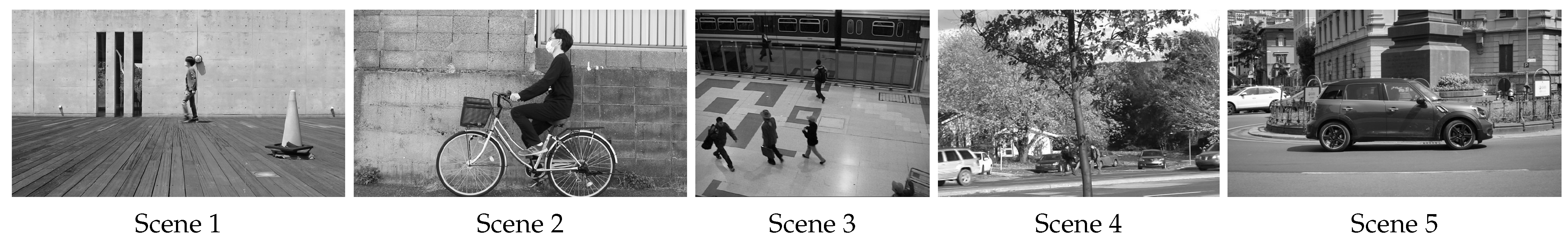
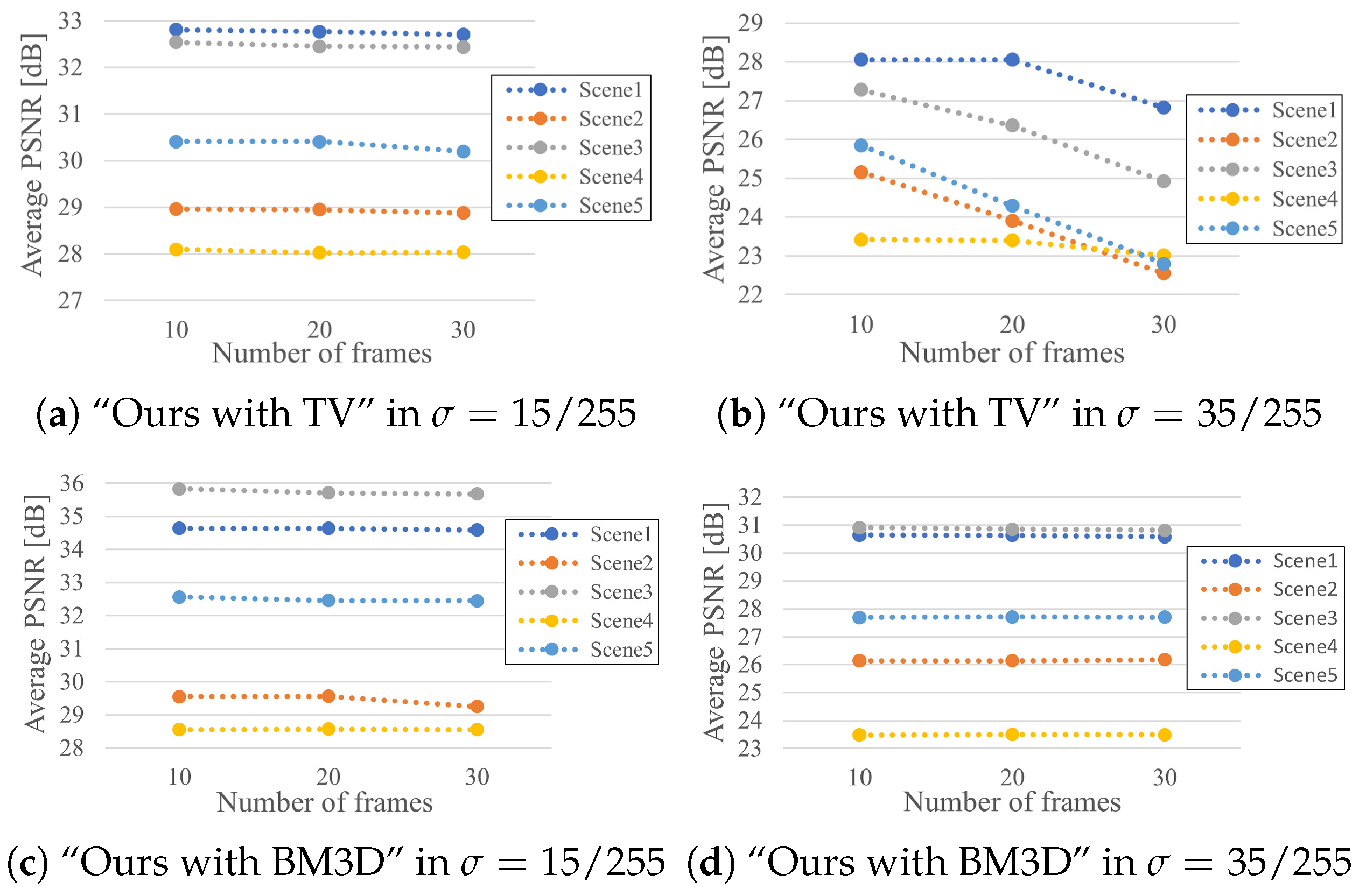
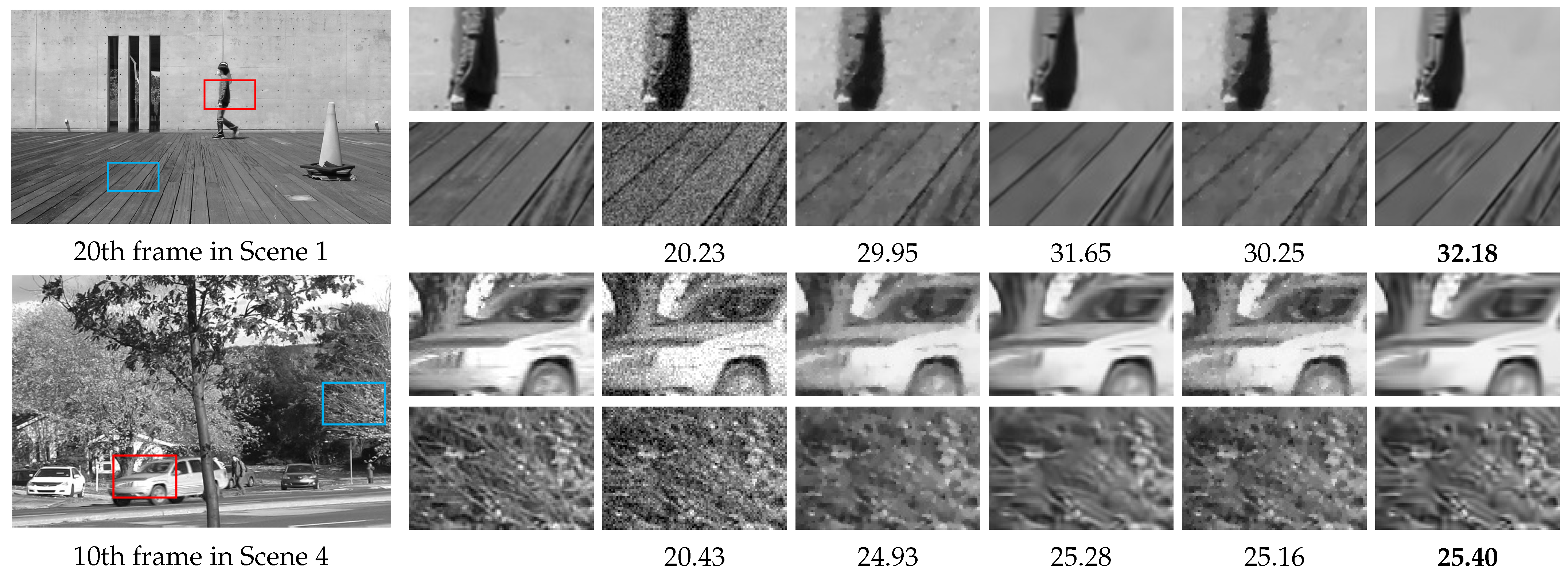
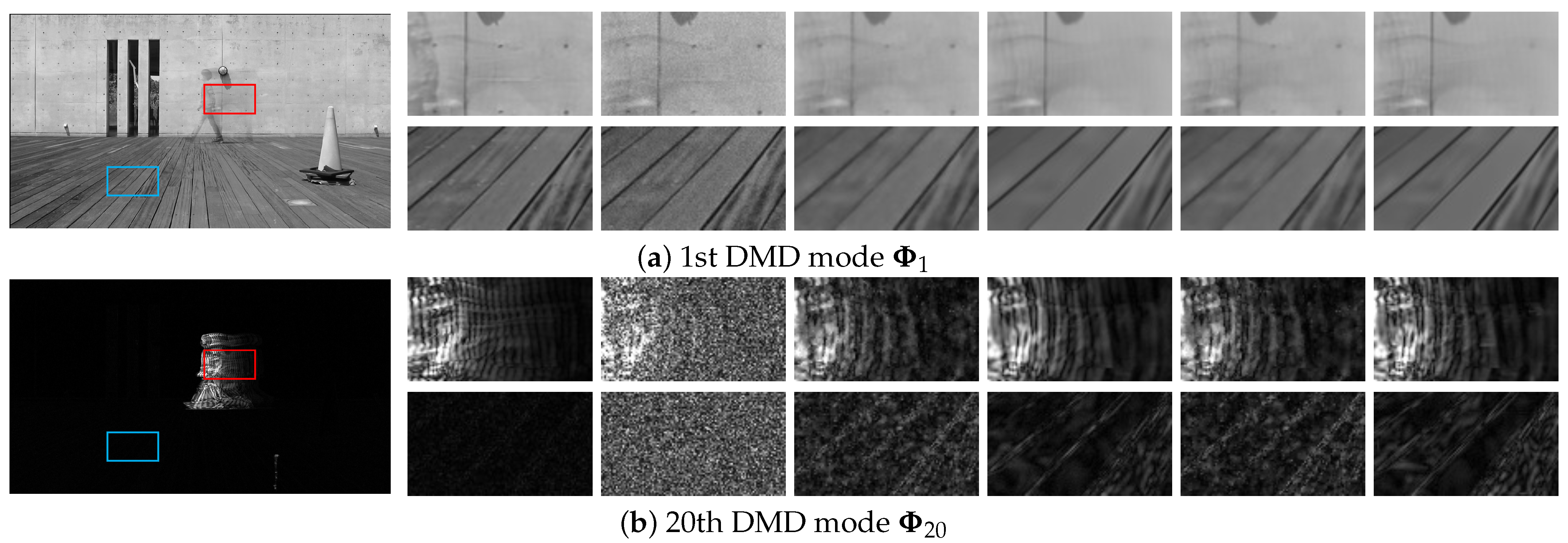
1:
Input Y ,   Z i ( 0 ) Θ i ( 0 ) , ρ i   ( i = 1 , 2 , 3 , 4 ) α ϵ
2:
Output Φ ( t )
3:
while A stopping criterion is not satisfied do
4:
    Φ t + 1 arg min Φ ρ 1 2 Z 1 ( t ) Φ B Σ Θ 1 ( t ) F 2 + ρ 2 2 Z 2 ( t ) Φ Θ 2 ( t ) F 2 + ρ 3 2 Z 3 ( t ) Φ B Σ Θ 3 ( t ) F 2 + ρ 4 2 Z 4 ( t ) Φ B Σ Θ 4 ( t ) F 2 ;
5:
    Z 1 ( t + 1 ) D R r , α / ρ 1 Φ ( t + 1 ) B Σ + Θ 1 ( t ) ;
6:
    Z 2 ( t + 1 ) D R m , ( 1 α ) / ρ 2 Φ ( t + 1 ) + Θ 2 ( t ) ;
7:
    Z 3 ( t + 1 ) P B Y , ϵ F Φ ( t + 1 ) B Σ + Θ 3 ( t ) ;
8:
    Z 4 ( t + 1 ) P R N × M Φ ( t + 1 ) B Σ + Θ 4 ( t ) ;
9:
    Θ 1 ( t + 1 ) Θ 1 ( t ) + Φ ( t + 1 ) B Σ Z 1 ( t + 1 ) ;
10:
    Θ 2 ( t + 1 ) Θ 2 ( t ) + Φ ( t + 1 ) Z 2 ( t + 1 ) ;
11:
    Θ 3 ( t + 1 ) Θ 3 ( t ) + Φ ( t + 1 ) B Σ Z 3 ( t + 1 ) ;
12:
    Θ 4 ( t + 1 ) Θ 4 ( t ) + Φ ( t + 1 ) B Σ Z 4 ( t + 1 ) ;
13:
    t t + 1 ;
14:
end while
The update of  Φ  in step 4 of Algorithm 2 is achieved by solving the quadratic minimization problem. The optimal solution satisfies the condition that the partial derivative of the following quadratic cost function with respect to  Φ  is zero (hereafter, the superscript  ( t )  is omitted for simplicity):
E Φ = ρ 1 2 Z 1 Φ B Σ Θ 1 F 2 + ρ 2 2 Z 2 Φ Θ 2 F 2 + ρ 3 2 Z 3 Φ B Σ Θ 3 F 2 + ρ 4 2 Z 4 Φ B Σ Θ 4 F 2 .
By setting the first-order derivative to zero, the optimal solution is determined by solving the system of linear equations:
Φ Ψ = Ξ , Ψ = ρ 1 B Σ Σ * B * + ρ 2 I + ρ 3 B Σ Σ * B * + ρ 4 B Σ Σ * B * , Ξ = ρ 2 ( Z 1 Θ 1 ) Σ * B * + ρ 2 ( Z 2 Θ 2 ) + ρ 3 ( Z 3 Θ 3 ) Σ * B * + ρ 4 ( Z 4 Θ 4 ) Σ * B * ,
where  I R M × M  is the identity matrix. The optimal solution is obtained by the inverse problem  Φ = Ξ Ψ 1 .
The updates of  Z 1  and  Z 2  in steps 5 and 6 of Algorithm 2 can be accomplished by employing the Gaussian denoiser  D R r , α / ρ 1  and  D R m , ( 1 α ) / ρ 2  as regularization terms  R r  and  R m , respectively. In our experiments, we utilized the TV algorithm discussed in Section 2.4 or BM3D [22] for both denoisers of  D R r , α / ρ 1  and  D R m , ( 1 α ) / ρ 2 . These Gaussian denoisers can restore smooth reconstructed frames and DMD modes while effectively removing noise.
The updates of  Z 3  and  Z 4  in steps 7 and 8 of Algorithm 2 require the computation of the proximity operators for the indicator functions of  ι B Y , ϵ F ( · )  and  ι R N × M ( · ) , which are equivalent to the metric projections onto them. Similar to Equation (13), the metric projection onto  B Y , ϵ F  is given by
P B Y , ϵ F ( X ) = X , if X B Y , ϵ F , Y + ϵ ( X Y ) X Y F , otherwise .
Then, the metric projection onto  R N × M  is given by  P R N × M ( X ) = real ( X ) , where  real ( X )  is the real part of  X .

4. Experiments

To demonstrate the effectiveness of the proposed method, we applied it to several noisy videos and compared it with naive noise removal methods in which the TV and BM3D denoisers were applied directly to the video frames. We refer to these methods as “naive TV” and “naive BM3D”. These results were obtained by setting  α  to 1, and these methods did not consider any regularization for the DMD mode. By comparing with such naive noise removal approaches, we can confirm the effectiveness of our proposed method that considers regularization for the DMD mode, namely the effectiveness of explicitly applying denoisers to the DMD mode. We refer to our method with the TV denoiser and the BM3D denoiser as “Ours with TV” and “Ours with BM3D”.
Figure 1 shows the original video scenes used for experiments. Scene 1 and Scene 2 videos were captured by the authors, Scene 3 and Scene 4 videos were selected from the SBMnet dataset [35], and Scene 5 video was selected from the DAVIS dataset [36]. We extracted  M = 10 , 20 , 30  [frames] from the first frame of each video. For the sake of simplicity, a color video was converted to grayscale. The details of each scene are briefly summarized as follows:
We independently added AWGN with three intensities, i.e.,  15 / 255 , 25 / 255 , and  35 / 255 , to input video frames. The visually best results with the proposed method were obtained by setting  ϵ = 0.95 N M σ 2  and adjusting the value of  α  from 0 to 1 in steps of  0.1 . For the quality metrics, we used the peak signal-to-noise ratio (PSNR) and the structural similarity index (SSIM) [37]. If the structure similarity between the input and reference images is high, the SSIM value is closer to 1 (for details, see [37]).
Table 1 and Table 2 show the average PSNR and SSIM of all frames obtained by the proposed and naive methods. In the cases of “Ours with TV” and “Ours with BM3D”, the values of  α  that yielded the best results are shown in brackets. One can see from Table 1 that “Ours with BM3D” has the highest average PSNR values compared to naive TV, naive BM3D, and “Ours with TV”. Then, one observes from Table 2 that “Ours with BM3D” has higher average SSIM values than the other methods in most cases. However, in Scene 2, “Ours with TV” tends to have higher values than the other methods. This is because BM3D cannot preserve the complex texture of the background concrete wall, and it is lost due to over-smoothing. Thus, the SSIM values of BM3D denoiser-based methods tend to be lower than those of TV denoiser-based methods. It has been observed that “Ours with TV” has higher PSNR and SSIM values than naive TV, regardless of noise intensity in the cases of  M = 10  and 20. However, in the case of  M = 30  and  σ = 35 / 255 , the values of “Ours with TV” are lower than those of naive TV. As frames increase, the DMD algorithm yields more DMD modes, including high-frequency modes representing fine vibrational components. The TV denoiser is suitable for improving spatial smoothness but does not preserve textures like repeating patterns. The estimated DMD modes by “Ours with TV” have fewer high-frequency components, so PSNR and SSIM values deteriorate.
Figure 2a,b illustrate the PSNR trends for “Ours with TV” under AWGN with  σ = 15 / 255  and  35 / 255 , respectively. They indicate that as the frame count rises, particularly under high noise levels, the performance of “Ours with TV” declines due to the increasing complexity of the DMD mode. The TV denoiser struggles to preserve minor DMD mode changes. Figure 2c,d demonstrate that “Ours with BM3D” maintains consistently high PSNR values, even with more frames and elevated noise levels. This stability is attributed to BM3D’s ability to exploit similar patches in the high-frequency DMD mode effectively. Similar trends were observed in the average SSIM values.
Figure 3 shows some close-ups of Scenes 1 and 4 degraded by AWGN with the standard deviation  σ = 25 / 255 . In Scene 1, “Ours with BM3D” and naive BM3D can remove noise, preserving the human silhouette, while “Ours with BM3D” shows superior preservation of wood fine texture. However, “Our with TV” and naive TV only partially restore sharp edges and textures. In Scene 4, “Ours with BM3D” and naive BM3D successfully remove noise while maintaining the car and wood silhouette, whereas “Ours with TV” and naive TV cannot restore sharp edges. Notably, “Ours with BM3D” outperforms naive BM3D in restoring tree edges and textures. Its direct noise removal in the DMD mode effectively preserves high-frequency modes even in areas with motion and complex textures.
Figure 4 shows some close-ups of the DMD mode of Scene 1 in the case of AWGN with  σ = 25 / 255 . This figure shows that “Ours with BM3D” can remove noise while preserving the edges and rich textures of the DMD modes  Φ 1  and  Φ 20 . The restoration results of naive BM3D can effectively remove noise similar to “Ours with BM3D”. However, due to the implicit restoration of the DMD mode, its restoration accuracy seems inferior to “Ours with BM3D”. In contrast, “Ours with BM3D” can restore the textures of the DMD mode more clearly than naive BM3D. This is because noise removal can be applied directly to the DMD mode, resulting in preserved edges and textures. Although “Ours with TV” can reduce noise better than naive TV, it is less effective at removing noise than both methods based on the BM3D denoiser, especially in the high-frequency mode  Φ 20 .
Next, we applied “Ours with BM3D” and “Ours with TV” to real noisy video captured with a high ISO setting in low light conditions and compared the results with those of naive TV and naive BM3D to show their effectiveness on real video. Figure 5 shows some close-ups of the resulting images with the gamma correction set to  γ = 1.3  for better visibility. This figure shows that “Ours with BM3D” effectively preserves the edge of the fence and has a better noise removal effect than naive TV, naive BM3D, and “Ours with TV”. Conversely, “Ours with TV” is better at preserving complex details, such as concrete wall patterns that are difficult to recover with the BM3D denoiser.
Finally, we discuss the computational cost of the proposed method. All experiments were conducted using MATLAB R2021a on a system equipped with an AMD EPYC 7402P 2.80 GHz processor and 128 GB RAM. Our method uses the iterative algorithm based on the PnP-ADMM framework, where each iteration requires a denoiser computation. The TV denoiser requires iterative computation using the ADMM algorithm (see Section 2.4 for details). Fortunately, as shown in the reference [21], it is possible to perform fast computations using the fast Fourier transform to solve the quadratic minimization problem with respect to  x  in Equation (16). Therefore, this denoiser can be executed in a relatively short computation time. The BM3D denoiser requires iterative computation using a non-local mean algorithm. Specifically, it is necessary to repeatedly search for many patches similar to the target patch from a wide range around it, which requires high computational cost and relatively long execution time. Figure 6 shows the average computational time when naive TV, naive BM3D, “Ours with the TV”, and “Ours with BM3D” on a video with an image size of  256 × 256 . The execution time when applying each method to a video with a frame size of 10 was as follows:
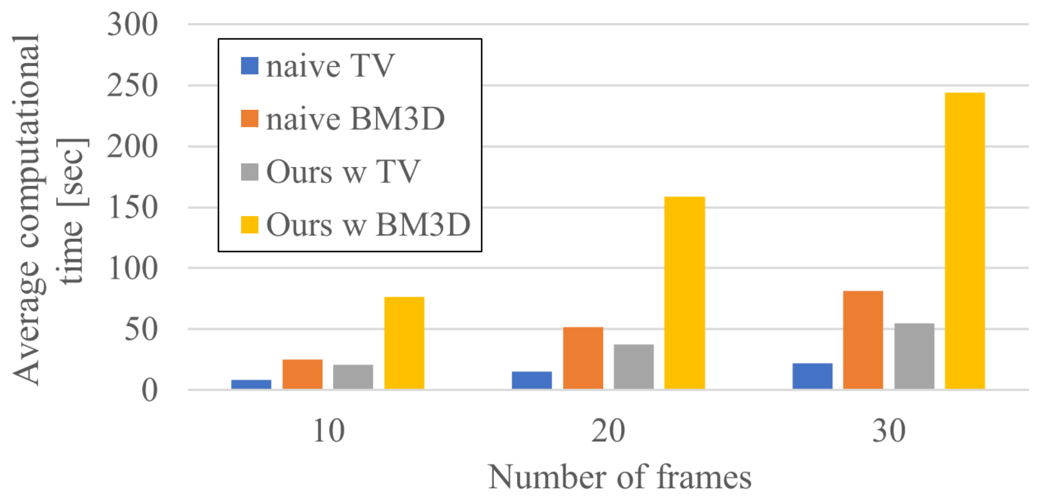
  • Naive TV was performed in less than 10 s.
  • Naive BM3D was performed in about 25 s.
  • “Ours with TV” was performed in about 20 s and shorter execution time than naive BM3D.
  • “Ours with BM3D” was performed in about 75 s and about three times slower than naive BM3D.
“Ours with BM3D” achieves the highest noise removal accuracy among the compared methods. However, it also requires a longer computational time. Despite taking roughly three times longer than naive BM3D, we still consider it practical. Furthermore, the figure illustrates that the computation time for each method increases proportionally with the number of frames.

5. Conclusions

In this paper, we introduced a novel noise removal method for the DMD mode of a noisy video. Specifically, the minimization problem that simultaneously reduces the noise of the DMD mode and the reconstructed video was defined. Then, we solved the proposed problem using the PnP-ADMM algorithm. The experiments confirmed that the proposed method can effectively remove noise in the DMD mode and the reconstructed video. These results suggest the potential to provide more reliable results in image recognition and object detection, especially in video surveillance and object tracking applications where foreground and background separation is essential. The proposed method consistently demonstrated effectiveness over naive noise removal methods throughout the experiments.
In future work, we will employ stochastic gradient descent algorithms to improve the computational efficiency of the proposed PnP-ADMM algorithm. We will also apply the proposed method to other high-dimensional volume data noise removal problems, e.g., hyperspectral and CT/MRI imaging.

Author Contributions

Methodology, H.Y., S.A. and R.M.; software, H.Y., S.A. and R.M.; validation, H.Y., S.A. and R.M.; formal analysis, R.M.; investigation, R.M.; data curation, R.M.; writing—original draft preparation, H.Y., S.A. and R.M.; writing—review and editing, R.M.; project administration, R.M.; funding acquisition, R.M. All authors have read and agreed to the published version of the manuscript.

Funding

This work was partially supported by JSPS KAKENHI Grant Number 21K17767 and MEXT Promotion of Distinctive Joint Research Center Program Grant Number #JPMXP 0621467946. The experiments in this paper were performed using DeeplearningBOX/Alpha Workstation at The University of Kitakyushu.

Data Availability Statement

Data will be shared with interested third parties on reasonable request.

Conflicts of Interest

The authors declare no conflicts of interest.

References

  1. Grosek, J.; Kutz, J.N. Dynamic mode decomposition for real-time background/foreground separation in video. arXiv 2014, arXiv:1404.7592. [Google Scholar]
  2. Kutz, J.N.; Fu, X.; Brunton, S.L.; Erichson, N.B. Multi-resolution Dynamic Mode Decomposition for Foreground/Background Separation and Object Tracking. In Proceedings of the IEEE International Conference on Computer Vision Workshop (ICCVW), Santiago, Chile, 7–13 December 2015; pp. 921–929. [Google Scholar] [CrossRef]
  3. Kutz, J.N.; Grosek, J.; Brunton, S.L. Dynamic mode decomposition for robust pca with applications to foreground/background subtraction in video streams and multi-resolution analysis. In CRC Handbook on Robust Low-Rank and Sparse Matrix Decomposition: Applications in Image and Video Processing; CRC Press: Boca Raton, FL, USA, 2016. [Google Scholar]
  4. Erichson, N.B.; Donovan, C. Randomized low-rank dynamic mode decomposition for motion detection. Comput. Vis. Image Underst. 2016, 146, 40–50. [Google Scholar] [CrossRef]
  5. Dicle, C.; Mansour, H.; Tian, D.; Benosman, M.; Vetro, A. Robust low-rank dynamic mode decomposition for compressed domain crowd and traffic flow analysis. In Proceedings of the IEEE International Conference on Multimedia and Expo (ICME), Seattle, WA, USA, 11–15 July 2016; pp. 1–6. [Google Scholar] [CrossRef]
  6. Pendergrass, S.; Brunton, S.L.; Kutz, J.N.; Erichson, N.B.; Askham, T. Dynamic Mode Decomposition for Background Modeling. In Proceedings of the IEEE International Conference on Computer Vision Workshops (ICCVW), Venice, Italy, 22–29 October 2017; pp. 1862–1870. [Google Scholar] [CrossRef]
  7. Takeishi, N.; Kawahara, Y.; Yairi, T. Sparse nonnegative dynamic mode decomposition. In Proceedings of the IEEE International Conference on Image Processing (ICIP), Beijing, China, 17–20 September 2017; pp. 2682–2686. [Google Scholar] [CrossRef]
  8. Bi, C.; Yuan, Y.; Zhang, J.; Shi, Y.; Xiang, Y.; Wang, Y.; Zhang, R. Dynamic Mode Decomposition Based Video Shot Detection. IEEE Access 2018, 6, 21397–21407. [Google Scholar] [CrossRef]
  9. Erichson, N.B.; Brunton, S.L.; Kutz, J.N. Compressed dynamic mode decomposition for background modeling. J. Real-Time Image Process. 2019, 16, 1479–1492. [Google Scholar] [CrossRef]
  10. Schmid, P.J. Dynamic mode decomposition of numerical and experimental data. J. Fluid Mech. 2010, 656, 5–28. [Google Scholar] [CrossRef]
  11. Mezić, I. Analysis of Fluid Flows via Spectral Properties of the Koopman Operator. Annu. Rev. Fluid Mech. 2013, 45, 357–378. [Google Scholar] [CrossRef]
  12. Kutz, J.N.; Brunton, S.L.; Brunton, B.W.; Proctor, J.L. Dynamic Mode Decomposition; Socoety for Industiral and Applied Mathemathics: Philadelphia, PA, USA, 2016. [Google Scholar] [CrossRef]
  13. Dawson, S.T.; Hemati, M.S.; Williams, M.O.; Rowley, C.W. Characterizing and correcting for the effect of sensor noise in the dynamic mode decomposition. Exp. Fluids 2016, 57, 42. [Google Scholar] [CrossRef]
  14. Hemati, M.S.; Rowley, C.W.; Deem, E.A.; Cattafesta, L.N. De-biasing the dynamic mode decomposition for applied Koopman spectral analysis of noisy datasets. Theor. Comput. Fluid Dyn. 2017, 31, 349–368. [Google Scholar] [CrossRef]
  15. Rudin, L.I.; Osher, S.; Fatemi, E. Nonlinear Total Variation Based Noise Removal Algorithms. Phys. D 1992, 60, 259–268. [Google Scholar] [CrossRef]
  16. Bresson, X.; Chan, T.F. Fast Dual Minimization of the Vectorial Total Variation Norm and Applications to Color Image Processing. Inverse Probl. Imag. 2008, 2, 455–484. [Google Scholar] [CrossRef]
  17. Chambolle, A. An Algorithm for Total Variation Minimization and Applications. J. Math. Imag. Vis. 2004, 20, 89–97. [Google Scholar] [CrossRef]
  18. Blomgren, P.; Chan, T.F. Color TV: Total variation methods for restoration of vector-valued images. IEEE Trans. Image Process. 1998, 7, 304–309. [Google Scholar] [CrossRef] [PubMed]
  19. Chan, S.H.; Khoshabeh, R.; Gibson, K.B.; Gill, P.E.; Nguyen, T.Q. An augmented Lagrangian method for total variation video restoration. IEEE Trans. Image Process. 2011, 20, 3097–3111. [Google Scholar] [CrossRef] [PubMed]
  20. Matsuoka, R.; Ono, S.; Okuda, M. Transformed-Domain Robust Multiple-Exposure Blending With Huber Loss. IEEE Access 2019, 7, 162282–162296. [Google Scholar] [CrossRef]
  21. Matsuoka, R.; Okuda, M. Beyond Staircasing Effect: Robust Image Smoothing via 0 Gradient Minimization and Novel Gradient Constraints. Signals 2023, 4, 669–686. [Google Scholar] [CrossRef]
  22. Dabov, K.; Foi, A.; Egiazarian, K. Video denoising by sparse 3D transform-domain collaborative filtering. In Proceedings of the 2007 15th European Signal Processing Conference, Poznan, Poland, 3–7 September 2007; pp. 145–149. [Google Scholar]
  23. Dabov, K.; Foi, A.; Katkovnik, V.; Egiazarian, K. Color image denoising via sparse 3D collaborative filtering with grouping constraint in luminance-chrominance space. In Proceedings of the 2007 IEEE International Conference on Image Processing, San Antonio, TX, USA, 16 September–19 October 2007; Volume 1, pp. 1–313. [Google Scholar]
  24. Maggioni, M.; Boracchi, G.; Foi, A.; Egiazarian, K. Video denoising, deblocking, and enhancement through separable 4-D nonlocal spatiotemporal transforms. IEEE Trans. Image Process. 2012, 21, 3952–3966. [Google Scholar] [CrossRef] [PubMed]
  25. Mäkinen, Y.; Azzari, L.; Foi, A. Collaborative filtering of correlated noise: Exact transform-domain variance for improved shrinkage and patch matching. IEEE Trans. Image Process. 2020, 29, 8339–8354. [Google Scholar] [CrossRef] [PubMed]
  26. Anami, S.; Matsuoka, R. Noise Removal for Dynamic Mode Decomposition Based on Plug-and-Play ADMM. In Proceedings of the 2021 Asia-Pacific Signal and Information Processing Association Annual Summit and Conference (APSIPA ASC), Tokyo, Japan, 14–17 December 2021; pp. 1405–1409. [Google Scholar]
  27. Tu, J.H. Dynamic Mode Decomposition: Theory and Applications. Ph.D. Thesis, Princeton University, Princeton, NJ, USA, 2013. [Google Scholar]
  28. Brunton, S.L.; Proctor, J.L.; Tu, J.H.; Kutz, J.N. Compressed sensing and dynamic mode decomposition. J. Comput. Dyn. 2015, 2, 165. [Google Scholar] [CrossRef]
  29. Gabay, D.; Mercier, B. A dual algorithm for the solution of nonlinear variational problems via finite element approximation. Comput. Math. Appl. 1976, 2, 17–40. [Google Scholar] [CrossRef]
  30. Venkatakrishnan, S.V.; Bouman, C.A.; Wohlberg, B. Plug-and-play priors for model-based reconstruction. In Proceedings of the IEEE Global Conference on Signal and Information Processing, Austin, TX, USA, 3–5 December 2013; pp. 945–948. [Google Scholar]
  31. Chan, S.H.; Wang, X.; Elgendy, O.A. Plug-and-play ADMM for image restoration: Fixed-point convergence and applications. IEEE Trans. Comput. Imag. 2016, 3, 84–98. [Google Scholar] [CrossRef]
  32. Moreau, J.J. Fonctions convexes duales et points proximaux dans un espace hilbertien. C. R. Acad. Sci. 1962, 255, 2897–2899. [Google Scholar]
  33. Combettes, P.L.; Pesquet, J.C. A proximal decomposition method for solving convex variational inverse problems. Inverse Probl. 2008, 24, 065014. [Google Scholar] [CrossRef]
  34. Duval, V.; Aujol, J.F.; Vese, L.A. Mathematical Modeling of Textures: Application to Color Image Decomposition with a Projected Gradient Algorithm. J. Math. Imag. Vis. 2010, 37, 232–248. [Google Scholar] [CrossRef]
  35. Jodoin, P.M.; Maddalena, L.; Petrosino, A.; Wang, Y. Extensive Benchmark and Survey of Modeling Methods for Scene Background Initialization. IEEE Trans. Image Process. 2017, 26, 5244–5256. [Google Scholar] [CrossRef] [PubMed]
  36. Pont-Tuset, J.; Perazzi, F.; Caelles, S.; Arbelaez, P.; Sorkine-Hornung, A.; Gool, L.V. The 2017 DAVIS Challenge on Video Object Segmentation. arXiv 2017, arXiv:1704.00675. [Google Scholar]
  37. Wang, Z.; Bovik, A.; Sheikh, H.; Simoncelli, E. Image quality assessment: From error visibility to structural similarity. IEEE Trans. Image Process. 2004, 13, 600–612. [Google Scholar] [CrossRef] [PubMed]
Figure 1. Input video scenes. Scene 1: A person walks in front of a simple stationary background. Scene 2: A bicycle passes in front of a complex stationary background. Scene 3: Some people walk in front of a simple stationary background. Scene 4: A car passes in front of a dynamic background. Scene 5: Background and foreground move simultaneously. The camera is not fixed.
Signals 05 00011 g001
Figure 2. Relationship between number of frames and PSNR of the proposed methods.
Signals 05 00011 g002
Figure 3. Experimental results of (top) the 20th frame in Scene 1 and (bottom) the 10th frame in Scene 4 and their PSNR values [dB]. The close-up images indicated by the red and blue boxes are shown as follows: (from left to right) reference frame, input frame, naive TV, naive BM3D, Ours with TV using the best  α , and Ours with BM3D using the best  α .
Signals 05 00011 g003
Figure 4. Results of the estimated DMD modes in Scene 1 (a Φ 1  and (b Φ 20 . The close-up images indicated by the red and blue boxes are shown as follows: (from left to right) reference frame, input frame, naive TV, naive BM3D, “Ours with TV” using the best  α , and “Ours with BM3D” using the best  α .
Signals 05 00011 g004
Figure 5. Results of the 20th frame in a real scene captured with high ISO setting. The close-up images indicated by the red and blue boxes are shown as follows: (from left to right) input frame, naive TV, naive BM3D, “Ours with TV” using the best  α , and “Ours with BM3D” using the best  α .
Signals 05 00011 g005
Figure 6. Average computational time measurement results.
Signals 05 00011 g006
Table 1. Average PSNR comparison.
Scene σ M = 10  [Frame] M = 20  [Frame] M = 30  [Frame]
Noisy Naive
TV
Naive
BM3D
Ours with
TV   ( α )
Ours with
BM3D   ( α )
Noisy Naive
TV
Naive
BM3D
Ours with
TV   ( α )
Ours with
BM3D   ( α )
Noisy Naive
TV
Naive
BM3D
Ours with
TV   ( α )
Ours with
BM3D   ( α )
115/25524.6232.2934.1432.81 (0.4)34.64 (0.1)24.6232.2733.0632.77 (0.5)34.64 (0.1)24.6232.2733.0532.70 (0.6)34.59 (0.1)
25/25520.2330.2131.8130.31 (0.8)32.24 (0.3)20.2330.2831.6530.25 (0.9)32.19 (0.3)20.2329.9531.6530.25 (0.9)32.18 (0.3)
35/25517.4528.5330.5028.06 (0.9)30.64 (0.5)17.4528.5330.4928.06 (0.9)30.63 (0.5)17.4527.5630.3626.82 (0.9)30.59 (0.6)
215/25524.6628.3729.4628.96 (0.5)29.55 (0.4)24.6628.3629.5028.95 (0.6)29.56 (0.6)24.6628.3728.7828.88 (0.8)29.25 (0.1)
25/25520.3226.3427.4726.55 (0.7)27.48 (0.8)20.3226.5227.0026.54 (0.9)27.28 (0.4)20.3226.2927.0426.02 (0.9)27.32 (0.4)
35/25517.5525.1826.0925.16 (0.9)26.14 (0.5)17.5525.0226.0023.91 (0.9)26.14 (0.5)17.5424.3426.0322.55 (0.9)26.18 (0.5)
315/25524.7631.8534.8032.54 (0.4)35.83 (0.1)24.7631.8534.7732.45 (0.6)35.71 (0.2)24.7632.2334.7332.44 (0.6)35.68 (0.1)
25/25520.4429.2532.7429.63 (0.8)33.08 (0.3)20.4429.5732.7429.61 (0.9)33.07 (0.3)20.4529.4132.7029.09 (0.9)33.03 (0.3)
35/25517.6427.5730.8027.28 (0.9)30.91 (0.7)17.6526.9230.7326.36 (0.9)30.86 (0.6)17.6525.6030.7224.92 (0.9)30.82 (0.6)
415/25524.7526.8428.4928.10 (0.3)28.55 (0.4)24.7426.9028.5128.02 (0.5)28.57 (0.6)24.7426.9128.5128.03 (0.6)28.55 (0.7)
25/25520.4324.3125.6625.17 (0.5)25.67 (0.7)20.4324.9325.2725.16 (0.8)25.27 (0.2)20.4324.9325.2825.16 (0.8)25.40 (0.2)
35/25517.6623.1623.3023.42 (0.8)23.49 (0.3)17.6623.4223.2523.40 (0.9)23.51 (0.3)17.6623.2423.2523.01 (0.9)23.50 (0.3)
515/25524.7130.0031.2230.41 (0.6)32.56 (0.2)24.7029.9931.1230.41 (0.7)32.46 (0.2)24.7030.3431.1230.20 (0.9)32.45 (0.2)
25/25520.4127.4329.2627.68 (0.8)29.67 (0.4)20.3927.6729.1827.57 (0.9)29.66 (0.3)20.3827.0929.1726.70 (0.9)29.65 (0.4)
35/25517.6425.9227.5525.85 (0.9)27.70 (0.7)17.6124.8127.6724.29 (0.9)27.72 (0.9)17.6123.3327.6622.80 (0.9)27.71 (0.6)
Table 2. Average SSIM comparison.
Scene   σ M = 10  [Frame] M = 20  [Frame] M = 30  [Frame]
Noisy Naive
TV
Naive
BM3D
Ours with
TV   ( α )
Ours with
BM3D   ( α )
Noisy Naive
TV
Naive
BM3D
Ours with
TV   ( α )
Ours with
BM3D   ( α )
Noisy Naive
TV
Naive
BM3D
Ours with
TV   ( α )
Ours with
BM3D   ( α )
115/2550.40920.85360.88570.8618 (0.5)0.8953 (0.1)0.40940.85360.86200.8609 (0.6)0.8955 (0.1)0.40950.85340.86170.8590 (0.7)0.8933 (0.1)
25/2550.23830.80420.83740.8044 (0.9)0.8502 (0.3)0.23810.80170.83230.7909 (0.9)0.8484 (0.2)0.23810.76130.83240.7904 (0.9)0.8480 (0.2)
35/2550.15910.72150.80770.6779 (0.9)0.8135 (0.5)0.15910.72220.80750.6783 (0.9)0.8133 (0.5)0.15920.63670.79290.5783 (0.9)0.8107 (0.7)
215/2550.61730.74650.77920.7865 (0.5)0.7822 (0.4)0.61970.75010.78330.7912 (0.6)0.7854 (0.6)0.62020.75140.73700.7887 (0.8)0.7659 (0.1)
25/2550.41910.65130.68420.6800 (0.7)0.6852 (0.8)0.42260.67600.64460.6824 (0.9)0.6687 (0.2)0.42330.67570.64870.6641 (0.9)0.6725 (0.2)
35/2550.30220.60310.59910.6084 (0.9)0.6045 (0.5)0.30620.60970.59390.5577 (0.9)0.6114 (0.5)0.30660.57950.59820.4961 (0.9)0.6159 (0.5)
315/2550.45410.88820.91230.8918 (0.6)0.9241 (0.1)0.45410.88790.91180.8903 (0.8)0.9216 (0.1)0.45560.88680.91150.8900 (0.8)0.9218 (0.1)
25/2550.29130.84490.89070.8445 (0.9)0.8966 (0.3)0.29130.83940.88970.8263 (0.9)0.8950 (0.5)0.29250.79690.88910.7633 (0.9)0.8940 (0.3)
35/2550.20820.75300.86580.7108 (0.9)0.8679 (0.5)0.20810.67280.86390.6200 (0.9)0.8661 (0.5)0.20880.56110.85540.5139 (0.9)0.8651 (0.5)
415/2550.76960.85400.89630.8876 (0.4)0.8965 (0.8)0.76760.85450.89660.8821 (0.5)0.8969 (0.6)0.76780.85450.89660.8863 (0.6)0.8972 (0.1)
25/2550.60690.76310.81740.8062 (0.5)0.8178 (0.1)0.60450.79550.79710.8050 (0.8)0.8175 (0.1)0.60430.79520.79710.8047 (0.8)0.8076 (0.2)
35/2550.48350.71770.70580.7365 (0.8)0.7530 (0.2)0.48130.73500.70320.7347 (0.9)0.7526 (0.2)0.48100.72550.70310.7138 (0.9)0.7523 (0.2)
515/2550.54650.87860.89900.8810 (0.7)0.9167 (0.1)0.54420.87660.89620.8774 (0.9)0.9141 (0.1)0.54570.85110.89560.8350 (0.9)0.9140 (0.1)
25/2550.38510.81860.86630.8142 (0.9)0.8761 (0.4)0.38210.79470.86280.7719 (0.9)0.8734 (0.3)0.38190.71750.86120.6849 (0.9)0.8725 (0.3)
35/2550.29140.74500.83190.7178 (0.9)0.8341 (0.7)0.28830.60490.82280.5676 (0.9)0.8310 (0.6)0.28740.51020.82050.4828 (0.9)0.8292 (0.5)
Disclaimer/Publisher’s Note: The statements, opinions and data contained in all publications are solely those of the individual author(s) and contributor(s) and not of MDPI and/or the editor(s). MDPI and/or the editor(s) disclaim responsibility for any injury to people or property resulting from any ideas, methods, instructions or products referred to in the content.

