1. Introduction
Real-time signal processing plays a predominant role in advanced industrial systems. Recently, the demand for high-speed signal processing for streaming data has significantly increased, especially in the fields of online surveillance, real-time communication, and intelligent control [
1,
2,
3,
4,
5]. Online analysis of streaming data can reveal valuable timely information about a system and allow rapid interventions.
Anomalies are patterns in data that differ substantially from an expected behaviour [
6,
7,
8]. There are two types of anomalies prevalent in time series data: point anomalies, where single data points do not comply with the neighbouring local pattern, e.g., a banking transaction of a much larger monetary value than a client’s norm, and collective anomalies, where groups of consecutive data points do not follow the general pattern, e.g., a period of reduced traffic intensity due to a car accident. Anomalies frequently arise in data as symptoms of undesirable events such as malicious activity, external attacks, emergencies, system faults, etc. Thus, detecting and diagnosing anomalies in a timely manner can help ensure the safety, efficiency, and optimality of critical systems [
1,
3,
5].
Traditionally, anomaly detection methods have been classified into three groups based on the level of external information provided:
supervised, where examples of previous (labelled) anomalies are used as a basis for detection;
unsupervised, where no such information is available and artefacts are identified purely on the basis of their deviation from the bulk of the data; and
semi-supervised, where some intermediate level of information is provided, e.g., labelling of portions of data that are definitively non-anomalous. Since supervised and semi-supervised approaches typically necessitate some human effort in segregating and labelling anomalies (which can be expensive and incompatible with large, streaming, multivariate data settings), much of modern anomaly detection, including this work, focuses on the unsupervised setting. However, most of the current unsupervised anomaly detection approaches fail on non-stationary signals, as the distribution of normal data points may shift with time but the approaches’ partitioning methods are static [
7,
8,
9]. Finally, it is worth mentioning in some other works [
3,
9,
10], which explored anomaly detection in nonlinear signals via data distribution estimation or next state prediction. These methods can handle the task of separating anomalies from a changing baseline. However, they do not address the problem of classifying and identifying the different types of anomalies for early intervention.
We propose a new three-part framework to
detect and cluster anomalies in non-stationary time series which can be used for unsupervised anomaly detection and analysis. We combine an online NARX (nonlinear autoregressive with exogenous input) detrending regime with anomaly detection (via SCAPA (sequential collective and point anomaly)) and a fuzzy clustering algorithm. NARX models are widely implemented due to their robust capabilities in the representation of complex systems that the standard ARIMA approaches cannot model [
11]. SCAPA [
12,
13,
14] simultaneously detects point anomalies and anomalous regions (
collective anomalies) in the detrended series via an efficient dynamic programming regime. Finally, collective anomaly segments can be clustered via fuzzy c-means clustering [
15] of their empirical distribution functions (ECDFs).
In summary, our main contribution is the provision of a method (for the first time, as far as we are aware) that considers the entire end-to-end process of
Detrending non-stationary time series,
Detecting anomalies in the residual series,
Grouping similar anomalies via fuzzy clustering.
Each phase uses state-of-the-art techniques from its requisite literature and can be applied effectively to multivariate series across various variants of non-stationarity and many classes of anomalous artefacts.
We provide a detailed empirical investigation of its efficacy using two datasets: the first, a year-long univariate nonlinear time series representing traffic on a telecommunications network, and the second, a multivariate real-data example from the Skoltech anomaly benchmark (SKAB) [
16] pertaining to systems control.
The remaining sections are organised as follows.
Section 2 outlines existing techniques and the main building blocks of our framework, while
Section 3 defines our integrated approach. Our empirical results, firstly for the detection phase, are presented in
Section 4, with a detailed consideration of the clustering aspect following in
Section 5,
Section 6 and
Section 7, before the final conclusions are presented in
Section 8.
2. Related Work
Anomaly detection is one of several common mining tasks for extracting meaningful knowledge from time series data [
9]. However, non-stationary time series pose significant challenges for anomaly detection as it is rather more difficult to detect and interpret anomalous changes from a moving series than a stationary one, especially in real time [
6,
7,
8]. Most existing methods can be categorised as identifying anomalies via model-based classification or statistical anomaly detection methods.
Model-based anomaly detection approaches can be further divided into two groups: estimation models and prediction models. Estimation models detect anomalies with the best-fit models, while prediction models focus on the prediction of the sequential states of the time series and can detect anomalies in an autoregressive way [
9,
17,
18]. All these model-based methods [
1,
3,
4,
5] rely heavily on accurately labelled training data to generate clusters of ‘anomalous’ and ‘normal’ data to which subsequent data are assigned. However, such labelled data are often expensive and hard to obtain in real time. Compared to our approach, these techniques retain little information on the structure of anomalies which would admit further analysis, such as clustering [
6,
7,
8].
Statistical anomaly detection methods mainly use density-based approaches or histogram-based approaches. Density-based anomaly detection methods are based on the concept of the neighbourhood, which is more complex for ordered data. Therefore, these methods are rarely used for temporal data. Histogram-based anomaly approaches create histogram representations of the original time series and remove anomalies to achieve lower error in these representations [
9,
10]. Statistical anomaly detection methods work in an unsupervised manner using, for instance, distribution-based clustering [
2,
19,
20]. However, these methods are limited by the assumption that the ‘normal’ behaviour is stationary or has a fixed periodic pattern which may be uncommon in practice [
6,
7,
8].
Our method carries the advantages of both approaches by first detrending the data and then applying anomaly detection on the (stationary) residual series, without the need for labelled ‘training’ anomalies. It has the additional advantage of being able to cluster multiple anomalies based on the distribution of the residuals within. We proceed to describe the constituent parts of our approach in more detail.
2.1. Nonlinear Autoregressive with Exogenous Input Model
A NARX model allows the combination of autoregressive modelling, regression on external series, and nonlinear basis functions, and are widely-used, versatile models for the analysis of complex time series [
21,
22,
23,
24]. We deploy NARX with neural basis functions favouring their flexibility, although other options such as polynomial or wavelet bases, sigmoid networks, etc., would be equally viable [
11].
The typical NARX neural network model relates a target series
to an exogenous series
in an autoregressive manner,
where
are the maximum lags for the series and
denotes additive noise [
11].
represents the basis function—in this case, the neural network—with a nonlinearity degree of
, defined by the complexity of the network.
NARX neural network models have been applied to meteorological prediction tasks [
25], simulation in health applications [
26,
27], and anomaly detection in industrial monitoring [
28,
29,
30]. However, previous anomaly detection schemes have used crude threshold exceedance-based criteria which can cope poorly with drifts and shifts in variance. Our combination of NARX with SCAPA (as described in the next section) adapts more readily to non-stationary data.
2.2. Sequential Collective and Point Anomalies
SCAPA [
13] is an online anomaly detection method which detects and distinguishes point and collective anomalies within time series with stationary baselines [
12].
In the univariate setting, where a series
follows some distribution
D, collective anomalies can be regarded as epidemic changes in parameters
away from normal parameters
[
12]. SCAPA identifies collective anomalies by minimising the following penalised cost over the number of collective anomalies
K, their start and end points,
and
, and normal feature parameters
[
12]:
where
is a cost function, and
is a penalty to prevent overfitting.
In our illustrative examples, we consider the mean and variance as our feature parameters and adopt twice the negative of the Gaussian log-likelihood as our cost function—a common choice, appropriate for our residual series. Within-anomaly parameter estimates
,
are not optimisation variables but are estimated by sample statistics within the set
. SCAPA has an efficient dynamic programming implementation in the R package
anomaly [
31]. We utilise this within our empirical examples with a minimum collective anomaly length of 2, a maximum anomaly length (chosen on a per-instance basis for computational efficiency), and a separate penalty
for point anomalies (which are regarded as changes in variance only, with a fixed length of 1).
3. Anomaly Detection and Clustering
This section outlines our proposed end-to-end framework for online anomaly detection and clustering, integrating the previously summarised components.
3.1. NARX-SCAPA
The detection component of the NARX-SCAPA framework uses a NARX neural network to provide a one-step-ahead prediction of the target time series in real time and then deploys SCAPA to identify anomalies in the prediction errors (residual) series. We have implemented this component via
NARX from
Neural Net Time Series App in Matlab R2021a [
32] and
SCAPA from R package
anomaly in CRAN [
31].
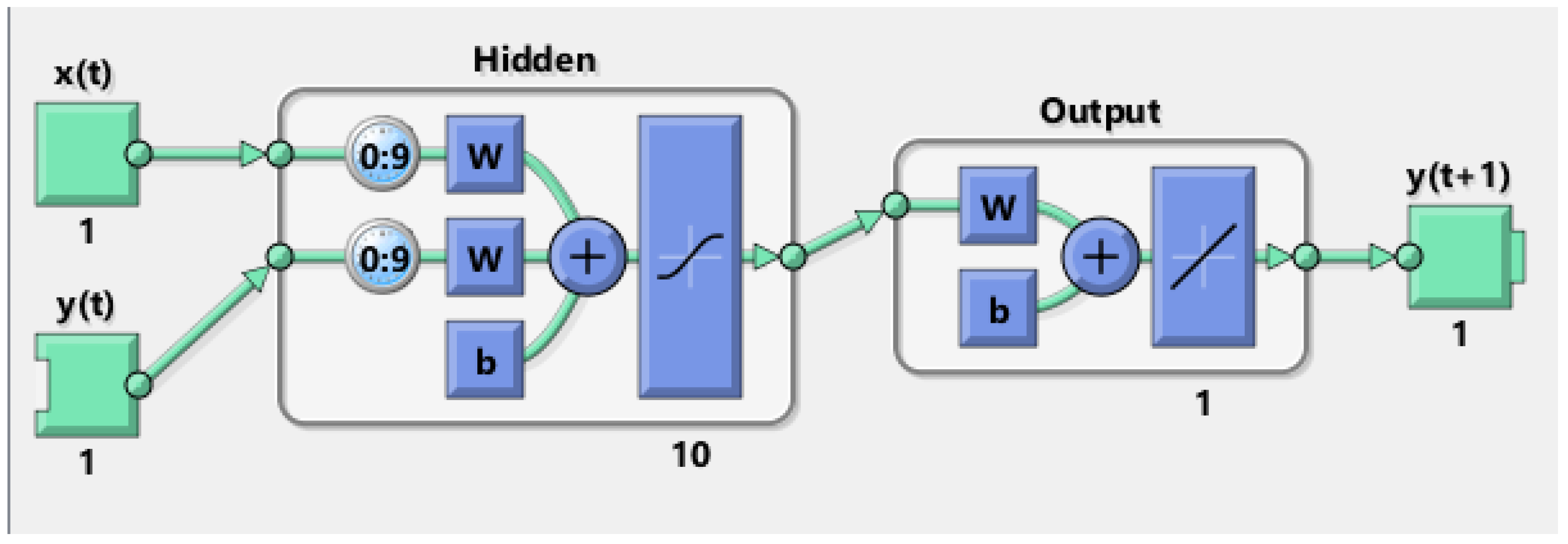
Figure 1 shows the example structure of the NARX neural network used to form a prediction
of the next point
based on the
n previous points and their corresponding time of day:
and
. The units in the hidden layer are based on the sigmoid function and the output layer uses a linear function of all hidden unit outputs. We use 1 hidden layer with 10 neurons and softmax for the output node, which follows the default setting of conventional neural networks that can balance the complexity and accuracy of the model in most cases. The operations within the hidden layer can be expressed as:
where
,
indexes the neurons, and
and
are the maximum lags considered in the model.
and
are the weights for the target time series and the exogenous series, respectively, and
represents the constant intercept. The output
s are passed through the final layer to form a prediction:
Once is observed, a residual is computed and reported as the next real-time observation to SCAPA.
Weights are estimated from an initial period of (assumed non-anomalous and complete) training data. We replace any missing observations and SCAPA-identified anomalous data from the (continuously evolving) input set with the prediction of the trained model.
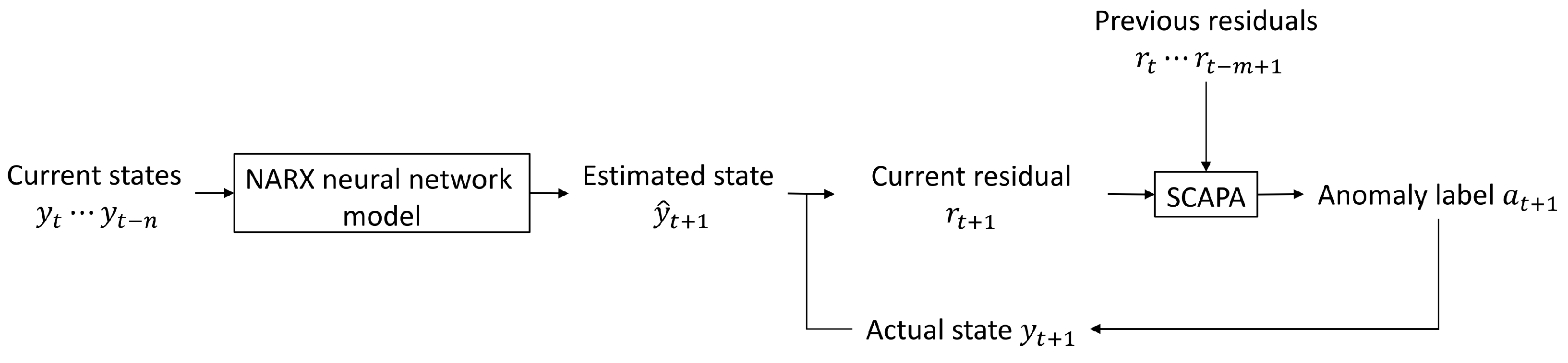
Figure 2 summarises the structure of the detection component.
The following steps summarise the overall detection mechanism:
Initialise a NARX neural network model with the training data;
Calculate the estimated value for the current time based on the actual observation values of the previous 10 s;
Calculate the current residual value between the estimated value and the actual observation when it is obtained;
Pass this residual as the next streaming observation to SCAPA to detect anomalies;
Label any points in the observation time series as anomalous if the corresponding residuals are identified by SCAPA;
Repeat steps 2 to 5 until the observation stops.
3.2. ECDF-Based Fuzzy c-Means Clustering
Once multiple anomalies are detected, we may follow up with clustering. We propose a method that represents anomalous segments (of potentially different lengths) by empirical cumulative distribution functions (ECDFs). Our ECDFs are discretized bins since fuzzy c-means clustering works well with vectors. The number of bins is of course adaptable, and for the subsequent experiments, 20 bins was chosen after exploratory analysis as a value which balanced the ability to capture the structure of anomalies with the ability to make reliable inference. The result is a ECDF vector associated with each anomaly , where for . Since we standardise the residuals to , we always have .
Fuzzy c-means clustering is a soft partitioning method whose output assigns each vector
,
a membership degree
for each cluster
such that
[
15].
The clustering is chosen as a solution to the optimisation problem:
where
D and
N are the numbers of ECDF vectors and clusters, respectively. The parameter
m is a fuzzy partition exponent for the degree of fuzzy cluster overlap and is set to be 2, based on the default setting of common fuzzy clustering. The
and
represent the
ith ECDF vector for anomalies and the
jth cluster centre vector.
The following steps explain the fuzzy clustering mechanism [
15]:
Randomly initialise the degree of membership .
Calculate the cluster centre vectors with:
Update the degree of membership using:
Compute with updated centres and membership degrees.
Repeat steps 2 to 4 until the distance between the old and new objective function is smaller than the minimum improvement threshold.
4. Detection Results
In this section, we illustrate the effectiveness of our approach on a telecommunications traffic dataset developed with BT.
4.1. Time Series Data
The BT network traffic data is a long-term non-stationary time series with a repeated daily pattern. It records traffic from BT’s network for continuous days at a sampling rate of 1 Hz. Within the data, some several anomalous points and regions do not follow the general distribution of the rest of the series, which in practice may only be partially identified and labelled by human experts and engineers or difficult to identify reliably at scale.
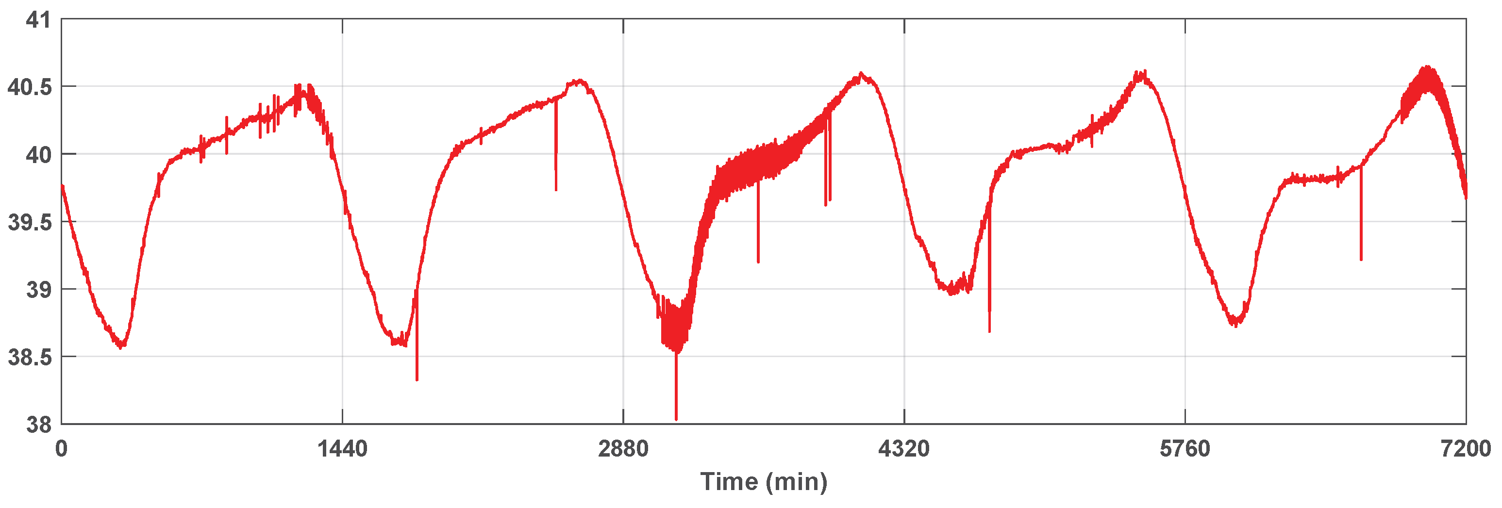
Figure 3 shows an excerpt of the time series from Day 1 to Day 5. The traffic follows a similar daily pattern due to the regular fluctuation of general uses but can include anomalies and noise on the daily level—as well as longer scale drifts and changes.
Drifts and shifts away from the established pattern as well as severe periods of interference are considered anomalies and can be consistently correlated with serious operational issues by engineers. As such, they often necessitate intervention, which may vary depending on the nature of the anomaly. Therefore, being able to detect and identify different anomalies in an online fashion plays a crucial role in maintaining the normal operational state of the network.
For confidentiality and to allow verification of our results, the bulk of our experimental work is based on a series simulated to have similar properties. We created a smooth series of 100 days of data to which we added artificial anomalies in known locations. The simulated series carries a similar daily fluctuation. The artificially introduced anomalies are also inspired by the structure of those manually labelled in the original series. Point anomalies are added by shifting random points up or down by a value sampled uniformly from . Our collective anomalies can be separated into three main types: (1) Splits: the trajectory of the time series splits into two or three parallel lines with spacing ± to for 100 to 200 min. (2) Interference: the variance of the time series significantly increases (5 to 10 times) for 75 to 250 min. (3) Shifts: the trajectory of the time series jumps to a different level and causes discontinuity, with to in amplitude and 0 to 10 times the original variance for 75 to 250 min.
The original series also exhibited anomalies that gradually returned to normal behaviour, as the intensity of the shift or interference slowly decrease (or decayed). These are particularly difficult to accurately detect. Based on these findings, we included 20 types of anomalies with intensities scaled between 0 and 1 in the simulation (see
Table A1 in
Appendix B for details). For each anomaly type, there are 10 instances randomly distributed over the entire simulated time series.
4.2. Online Anomaly Detection
The number of neurons in the hidden layer of NARX neural network models was set to be 10, and the maximum lags were also taken to be 10. With the BT network traffic data, the time of day in minutes (i.e., 1 to 1440) was introduced as the exogenous series (with a time delay
). The NARX model was fitted to five days of training data from the original series by optimising the weights
w and constants
b with Levenberg–Marquardt backpropagation [
33].
For SCAPA, we set the minimum and maximum segment lengths of collective anomalies to be and , respectively, for the BT network traffic data, and the penalties for collective and point anomalies to be and , respectively. These choices ensured that all known anomalies in the training data perfectly matched the sets of detected anomalous points, including the long (and decaying) collective anomalies.
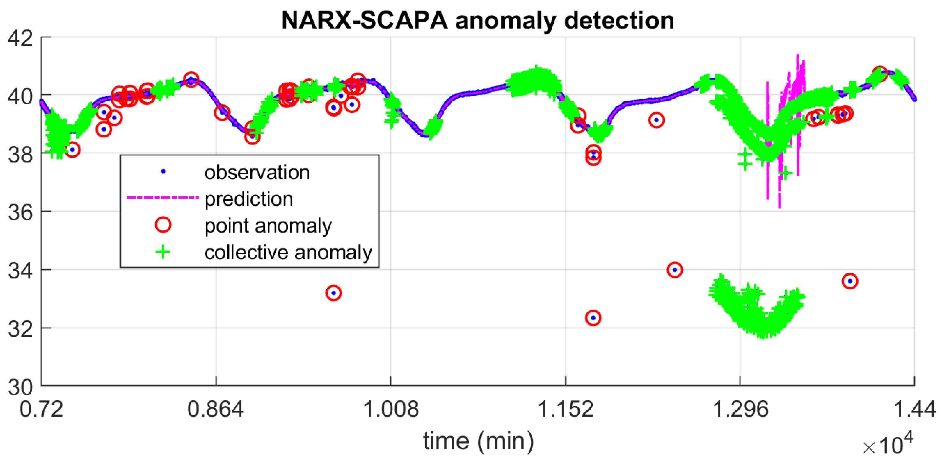
Figure 4 shows the results of implementing NARX-SCAPA on the first 10 days of the simulated traffic series with these settings. We see the NARX component’s success in capturing the typical non-stationary pattern and generating residual series where anomalies can be detected by SCAPA. It can be observed that all the anomalies were correctly identified and labelled, even for the point anomaly around 7500 min and the collective anomaly around 8800 to 9200, which were hard to identify by eye alone but are easily observed in the residual series.
In the full 100 days of simulated data, we introduced a total of 24,750 data points across 160 collective anomalies NARX-SCAPA identifies a total of 22,971 points within collective anomalies, 20,569 of which match with the design. The success of detection was significantly influenced by the intensity of an anomaly and the shape of the nonlinear series at the location of the anomaly, e.g., collective anomalies which commenced at a turning point of the series were hard to detect since the contrast to the regular series was minimal.
Meanwhile, since the intensity of anomaly points declined in the tails of decaying collective anomalies, the data points towards the end of a decay anomaly were likely to be neglected by the algorithm for lack of signal strength. Also, for some regions with relatively low-intensity collective anomalies, the NARX neural network was able to predict them as if they were normal parts of the time series. As a consequence, the residual series failed to provide any structural information about correlated collective anomalies in these regions and the SCAPA failed to label them as anomalies properly.
Table 1 summarises the collective anomaly detection results of the NARX-SCAPA. Anomaly regions with low or declining intensity, such as Type 13 to Type 18, were more difficult for the model to detect. However, the overall performance of the NARX-SCAPA model shows efficacy and efficiency in detecting and identifying various anomalies within non-stationary time series in real time. Similarly, there were a total of 40 point anomalies introduced into the simulated time series, of which NARX-SCAPA detected 33, with no false positives. Again, the success of detection depended on the intensity of the anomaly, as the breakdown by type shows.
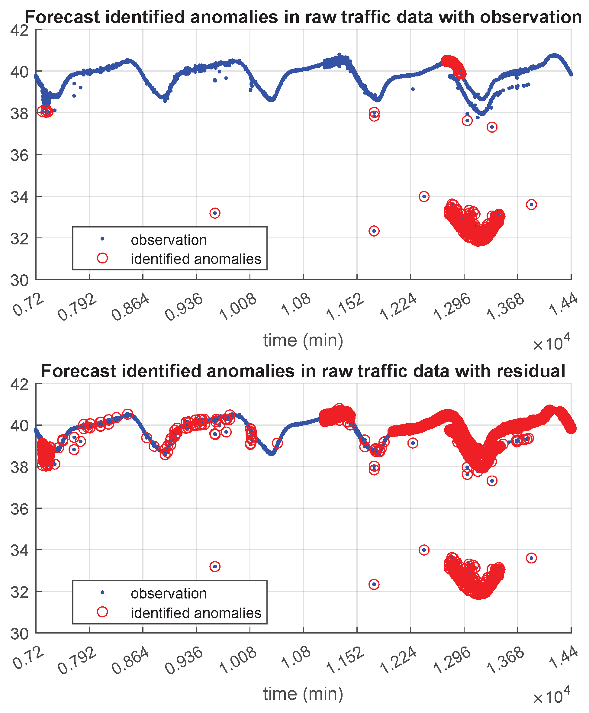
4.3. Real System Implementation
We also illustrate the performance of NARX-SCAPA on the original (i.e., not simulated) time series. Again, the model shows success at one-step ahead prediction in non-anomalous regions, and anomaly detection based on residuals. The NARX neural network was capable of handling the non-stationary time series and was adaptive to fluctuations within the normal range. Moreover, the model remained robust to the impact of severe anomalies, e.g., the regions around 7300, 11,000, and 13,000 min, where the observations were scattered, interfered, and split, respectively. The structures and the intensities of these anomalous regions were retained in the detrended residual series. However, it can also be seen in
Figure 5 that the prediction of the NARX-SCAPA-based model was distorted between 13,250 to 13,400 min, and this was due to the limitation of the NARX model and the long duration of strong anomalies. Yet, such distortions of the model prediction in the anomaly region were not able to compromise the detection of anomalies, as seen in
Figure 5. We see success in detecting point and collective anomalies, including those low-intensity anomalies which are hard to observe by eye alone.
4.4. Alternative Approaches
We compare the performance of NARX-SCAPA with two popular, existing alternatives from the R packages
Forecast and
HDoutlier. The
Forecast package, based on the model estimation method, is a commonly used tool for analysing large numbers of univariate time series in real time [
34]. It uses the
tsoutliers method to model univariate non-stationary time series via Multiple Seasonal-Trend decomposition using Loess (MSTL) and Friedman’s super smoother [
35]. Possible anomalies are identified within the two most extreme quartiles of the residual series. The
HDoutlier method allows probabilistic labelling of anomalies [
36]. The method partitions data into different exemplars according to the length of the series. It then computes nearest-neighbour distances between exemplars and fits the cumulative distribution function and labels data points in any exemplar that is far from the others as anomalies.
Table 2 and
Table 3 numerically compare the performance of these alternatives to NARX-SCAPA on the simulated data, both applied directly to the raw data and to the detrended residuals. We see that
Forecast was more suitable for the residual series, and
HDoutlier performed similarly in both cases. However, neither can achieve the same accuracy as NARX-SCAPA for detecting collective anomalies.
HDoutlier achieved high accuracy for point anomalies, but this was coupled with an extremely high false positive rate.
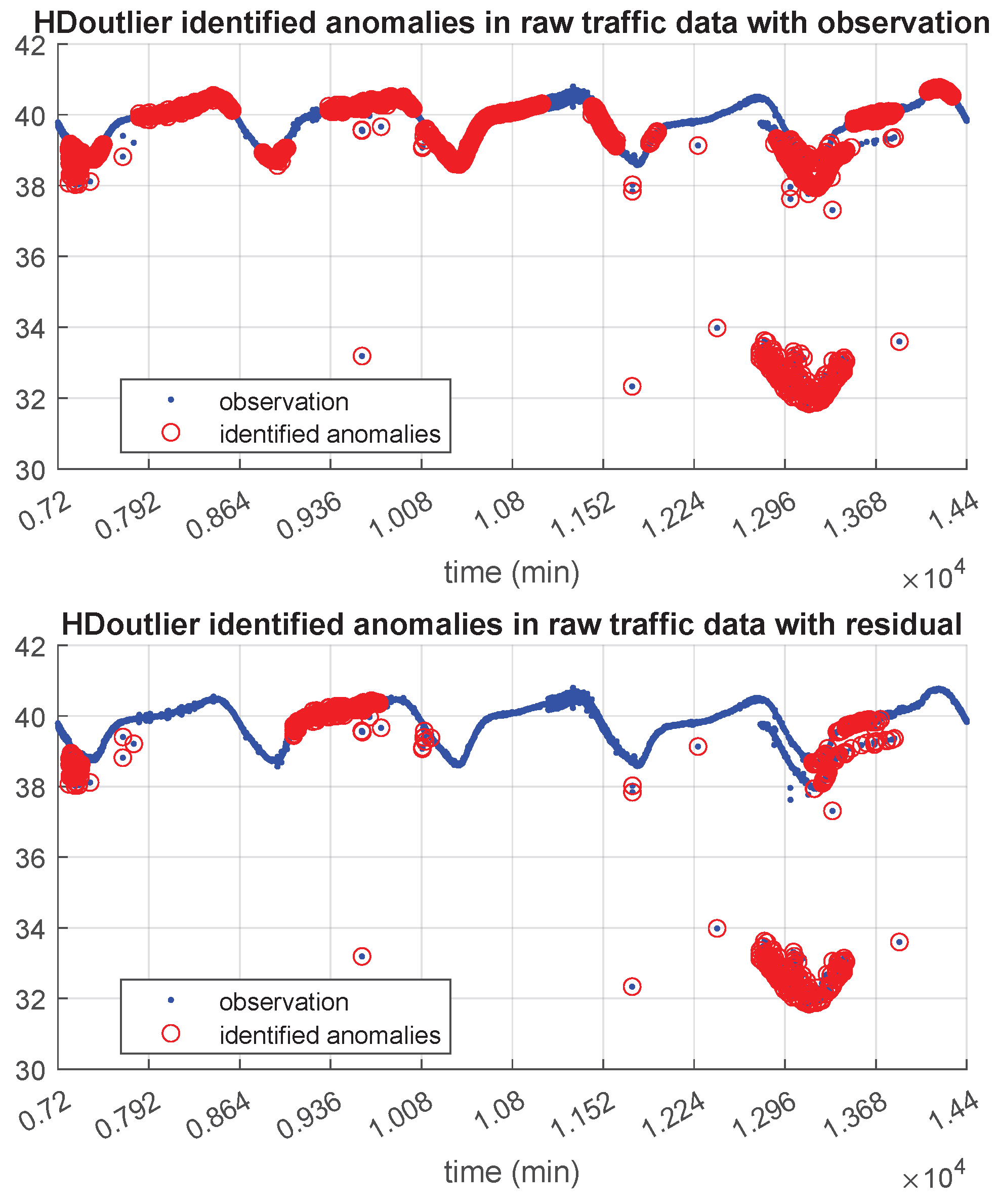
Figure A1 and
Figure A2 in
Appendix A provide a fuller visualisation and discussion of the results of implementing
Forecast and
HDoutlier approaches on the original BT network traffic data. We see that the
tsoutliers algorithm was overly sensitive in handling the residuals, and
HDoutliers was more conservative. It is worth noting that, for the BT traffic data, the probability of anomalies is low, yet their intensity is high. Therefore,
Forecast does not work well with a fixed strength of seasonality for the decomposition. Meanwhile, collective anomalies of the split Type remain a challenge for
HDoutliers as it either treats the outer data points as anomalies or labels entire regions as anomalies with a high false positive rate.
Overall, compared to the performance of
Forecast and
HDoutlier, the proposed NARX-SCAPA model has achieved the best anomaly detection results with minimal false positives and false negatives (see
Table 3).
5. Offline Anomaly Clustering
In this section, we consider the problem of clustering the detected collective anomalies based on the residuals. Clustering collective anomalies of different lengths based on their intensity and structure is a non-trivial task in itself, without an online approach. Therefore, we first normalise the original residual sequences with different distributional summaries (histogram and ECDF). Then, since the clustering usually depends on the distances between the targets, we explore two distance measures (Jensen–Shannon divergence and Euclidean distance), and finally, we compare various partitioning schemes (hierarchical clustering, k-means clustering, fuzzy c-means clustering, EPmeans and HMCluster).
5.1. Known Cluster Numbers
We deploy these combinations to cluster anomalies detected from running NARX-SCAPA on the simulated data, with the constraint that they should find 16 clusters. We compare performance across methods via the Rand index [
37] which counts the proportion of points allocated to the ‘correct’ cluster for their anomaly type. While the true anomaly type for each anomalous point is known to us, the clustering algorithms approach the problem as an unsupervised one and there are false positives among the anomalous points. Thus, to compute a performance measure, such as the Rand index, we must associate each cluster obtained with an anomaly type 1–16. This is achieved via a linear assignment algorithm [
38] which chooses an anomaly type to associate with each cluster, based on the proportions of each anomaly type therein.
The clustering algorithms take vectorised distribution summaries as their input, rather than the (variably sized) sets of residuals within each collective anomaly. We consider a histogram (or bin-wise frequency) summary and a discretised empirical cumulative distribution function (ECDF). Within the clustering algorithms, we compare two distance measures: the Jensen–Shannon divergence and the Euclidean distance. Under the hierarchical clustering, the histogram method achieves a Rand index of with the Jensen–Shannon divergence and with the Euclidean distance, and the ECDF method has a Rand index of with Jensen–Shannon divergence and with Euclidean distance.
We therefore argue that with hierarchical clustering, compared to Euclidean distance, Jensen–Shannon divergence is a more suitable measurement for the similarity of two probability distributions. We did however find that it was more sensitive to the granularity of the discretisation, with overly coarse choices leading to unreliable results, while the algorithm using Euclidean distance remained more robust. Furthermore, due to the complexity of differentiation within the expectation-maximisation iteration, Jensen–Shannon divergence cannot be directly combined with partitioning-based clustering algorithms, e.g., k-means clustering and fuzzy c-means clustering. Meanwhile, we see in
Table 4 that the ECDF works better than histogram with various clustering methods in distinguishing different types of collective anomalies in time series.
Next, we have compared the performances of three commonly used clustering algorithms with Euclidean distance: hierarchical clustering, k-means clustering and fuzzy c-means clustering. K-means clustering is a well-known spatial clustering algorithm that bases on the expectation-maximisation iteration to compute k clusters with all data points assigned to their nearest cluster centroids [
39]. Hierarchical clustering builds on the hierarchy of clusters that either merge or split data points with dendrograms [
40]. In addition, we have also applied two state-of-the-art clustering methods that were specifically designed for time series clustering: EPmeans and HMCluster. EPmeans is a non-parametric clustering approach that combines the Earth Mover’s Distance and k-means clustering for clustering probability distribution based on empirical cumulative distribution function (ECDF) [
41]. HMCluster is a spectral theory-based hierarchical method for identifying time series with total variation distance [
42]. The clustering performances using different distribution summaries and clustering methods are summarised with the Rand index in
Table 4.
The partitioning-based clustering methods—k-means clustering, fuzzy c-means clustering and EPmeans—have outperformed the tree-based clustering methods—hierarchical clustering and HMCluster. It is worth noting that hierarchical clustering is sensitive to noise and outliers. Meanwhile, for handling clusters with different sizes, hierarchical clustering tends to split large clusters and merge small clusters. Meanwhile, the results in
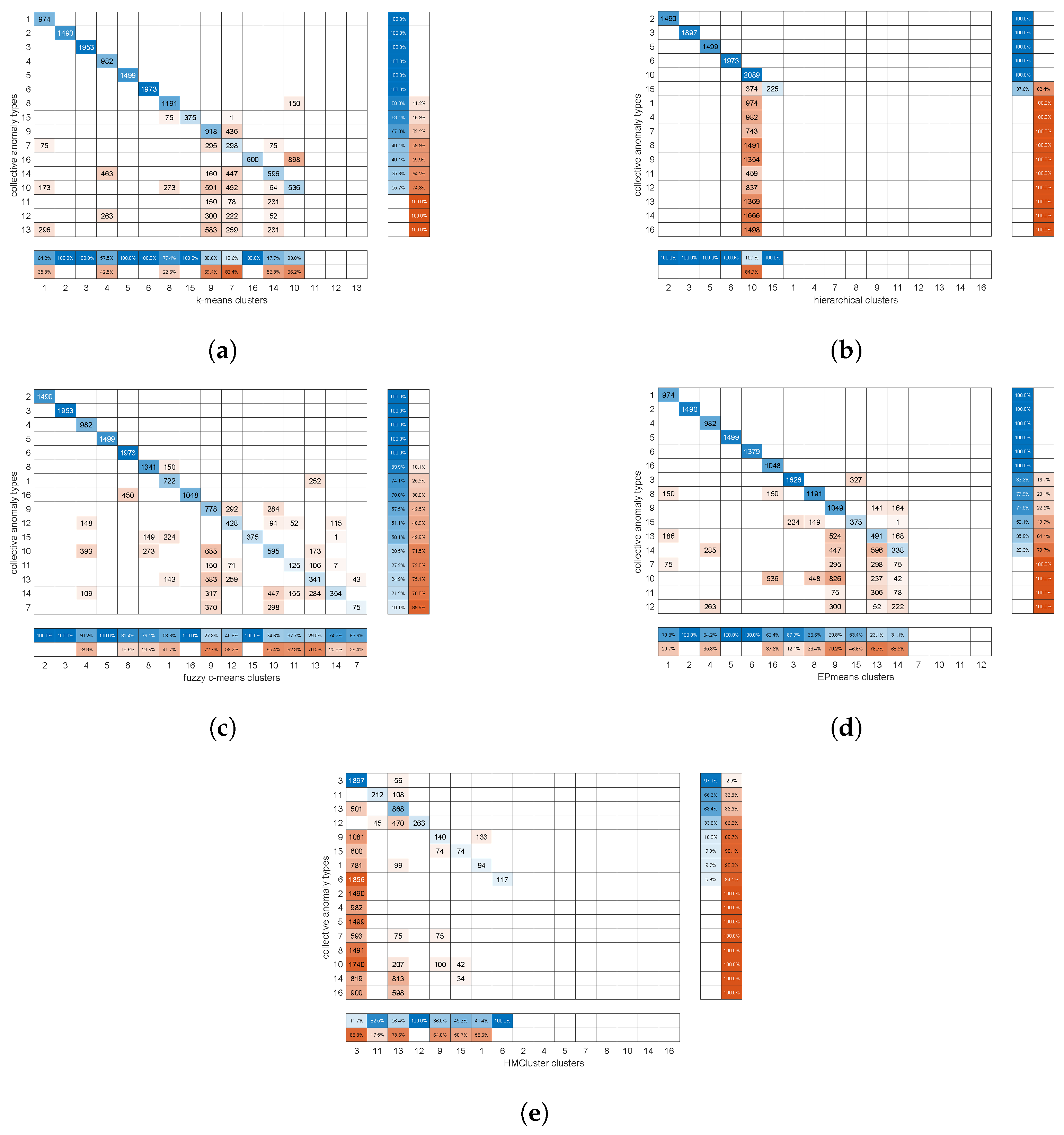
Table 4 show that, compared to the histogram, an ECDF can directly reflect the structures of time series segments without binning bias and be more robust to the outliers. Therefore, the ECDF appears to be a more suitable distribution summary for clustering collective anomalies. Compared to the other methods, the fuzzy c-means clustering with ECDF has achieved the best results for identifying all 16 types of anomalies with the least error rates. We summarise the clustering results using ECDF with confusion matrices in
Figure 6a–e, which allows for a more detailed comparison of different clustering methods.
Fuzzy c-means clustering with ECDF has outperformed other clustering methods, especially for differentiating shifts with small intensity from the interference (seeing
Figure 6c). EPmeans has achieved the second-best accuracy, only having some issues mixing the interference and the splits as in
Figure 6d. As shown in
Figure 6a, conventional k-means clustering shows reasonable clustering results, successfully dividing segments with different structures but still failing to differentiate the anomalies with varying intensity. Hierarchical-based clustering methods give the worst outcome as they could neither differentiate based on structure nor intensity of anomalies, as seen in
Figure 6b,e.
5.2. Sensitivity to Algorithm Parameters
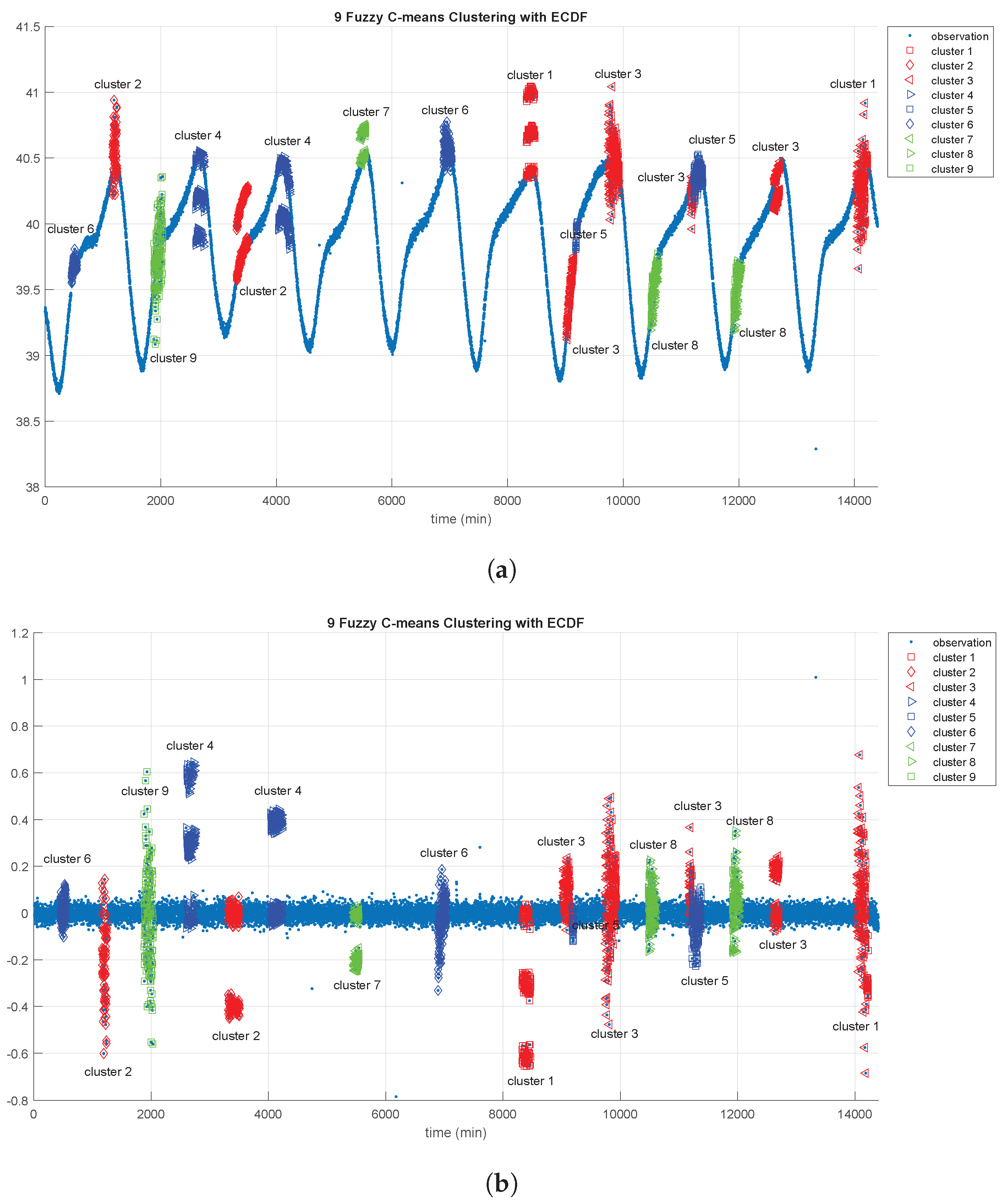
To assess the sensitivity of the ‘optimal’ clustering methodology—fuzzy c-means clustering with ECDF using Euclidean distance—we conduct further tests on the simulated time series with an assumption of nine clusters.
Figure 7 illustrates the results on 10 days of the series. We see that the three main categories of collective anomalies—split, interference, and shift—are appropriately distinguished. This suggests that the combination of fuzzy c-means clustering and ECDF is an effective way to cluster anomalous time series segments.
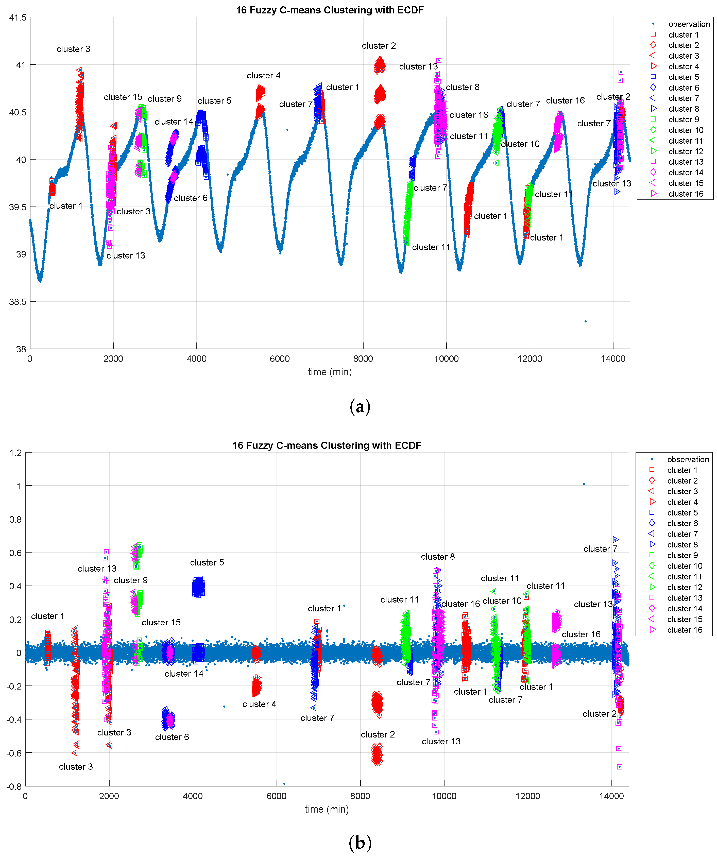
The maximum anomaly length of SCAPA is another key tunable parameter, so we experiment with it reduced to 60. This is less than the true maximum length and thus collective anomalies in the simulated time series may be sliced into multiple segments or shortened by SCAPA missing out the tails.
Figure 8 illustrates the results with the reduced maximum anomaly length and its resultant fragmented anomalies. We see a more pronounced detrimental effect as a result of the fragmentation. Principally, this is because tails of decaying anomalies were ignored or assigned to different anomaly segments by SCAPA, and points from the same anomaly type can seem to belong to very different patterns. Nevertheless, fuzzy c-means clustering with ECDF is able to cluster the most segments with similar structures together correctly, except for the region around 3250 min, where there is a change of nonlinear pattern for the time series.
Generally, we see that fuzzy c-means clustering and ECDF is an effective clustering method that can perform well with fragmented anomalous time series segments. It is more sensitive to the structural information rather than the general intensity of data distributions. Consequently, its performance was robust to some misspecification of the number of clusters but is slightly compromised with the misspecification of segment length.
6. Online Anomaly Clustering
In this section, we propose an integration of NARX-SCAPA and the ECDF-based fuzzy c-means clustering, so that anomalies can be clustered online. Such access to real-time clustering of anomalies can help decision-makers to diagnose and act on a system more effectively by making associations with previous anomalies.
We test the real-time clustering of collective anomalies with clusters from fuzzy c-means clustering using ECDF in a simple clustering/allocation scheme. First, we evenly divide the 20-day time series data into a training group and a testing group. Next, we detect the collective anomalies within the entire training group using the NARX-SCPA framework, and based on the results, we generate anomaly clusters with the ECDF-based fuzzy c-means clustering offline. Then, we implement the same anomaly detection method on the testing group in real time, and when a new anomaly sequence is fully detected, it is assigned to the nearest cluster in terms of the Euclidean distance.
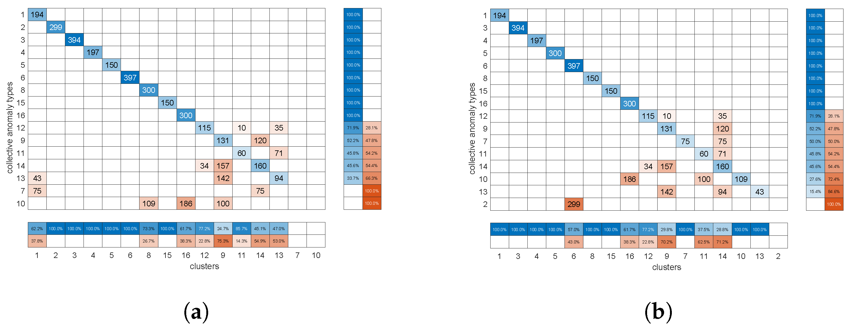
The results of such a clustering/allocation scheme are compared to the clustering results of fuzzy c-means clustering using ECDF with all anomalous time series segments from the 20-day simulated time series. It can be found in
Figure 9 that the performance of the clustering/allocation approach is similar to the clustering performance of fuzzy c-means clustering with ECDF, with Rand indices of
versus
. It suggests that such a clustering/allocation scheme is capable of online anomaly clustering with fuzzy c-means clustering, Euclidean distance, and ECDF. However, it is also worth noting that an increase in the amount of training data in the clustering stage can help the clustering with more generalised high-quality clusters that can accommodate more possible individual differences between the anomalies of the same type.
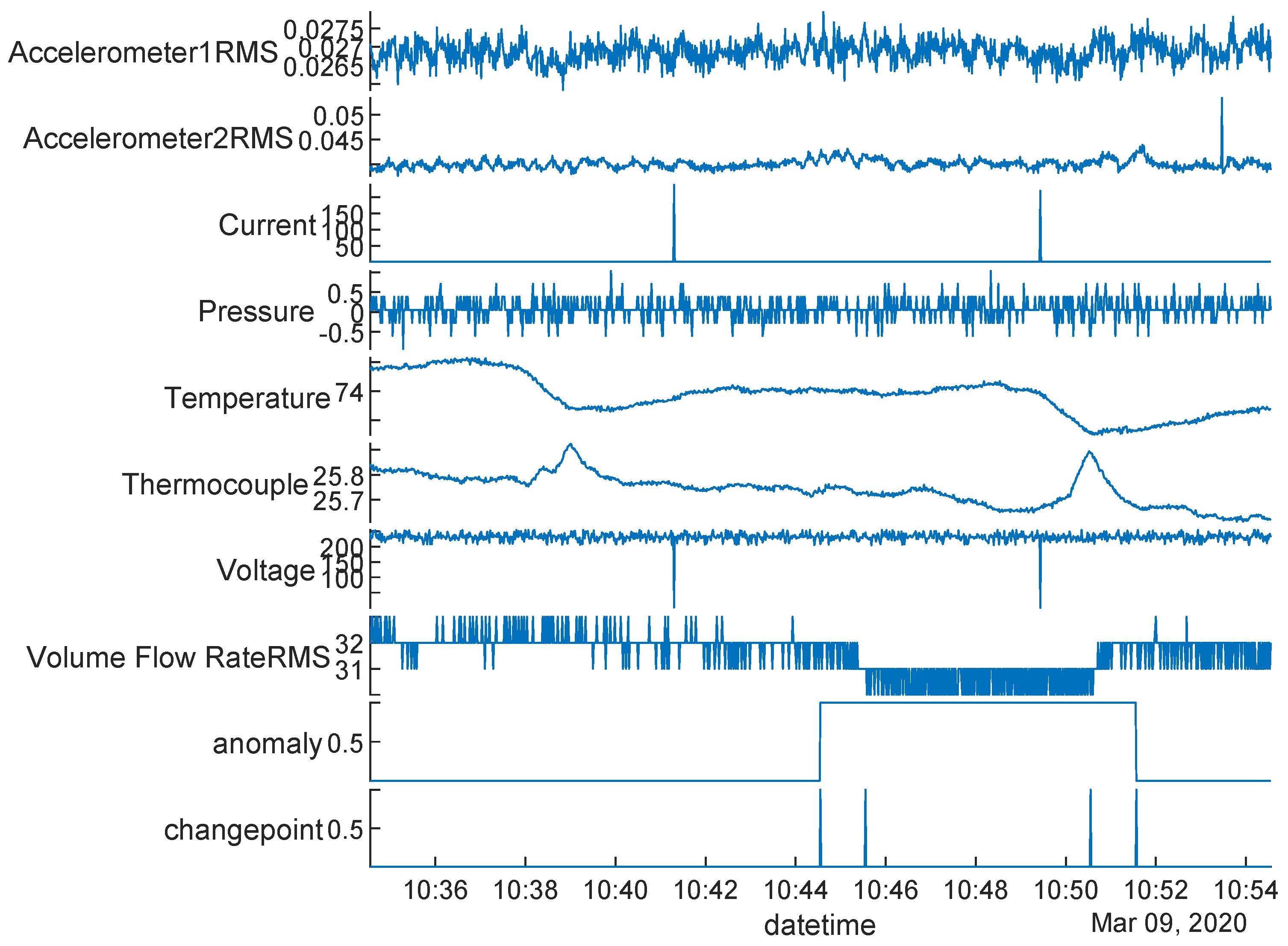
7. Multichannel Data
The Skoltech anomaly benchmark (SKAB) contains multichannel time series for evaluation of anomaly detection algorithms [
16]. It consists of multiple instances of multivariate series associated with eight sensors monitoring conditions on an IIot testbed and two additional series indicating the presence of anomalies and change points, as illustrated in the example in
Figure 10.
To model each channel of SKAB, we use the time series of other channels as the exogenous series to predict the target time series (also with the time delay
). Again, the model is optimised with Levenberg–Marquardt backpropagation. The anomaly-free instances in SKAB are used as training data for the modelling. Meanwhile, the minimum and maximum segment lengths of collective anomalies are
and
, respectively, and the penalties for collective and point anomalies to be
and
, respectively. The parameter settings are tuned to ensure no labelling of non-anomalous data as anomalous. To cluster, we use fuzzy c-means clustering with ECDF and optimise for three clusters. There are a total number of 7826 data points within collective anomalies across a total of 22,274 data points in SKAB. NARX-SCAPA identifies 5698 of these, achieving an accuracy of
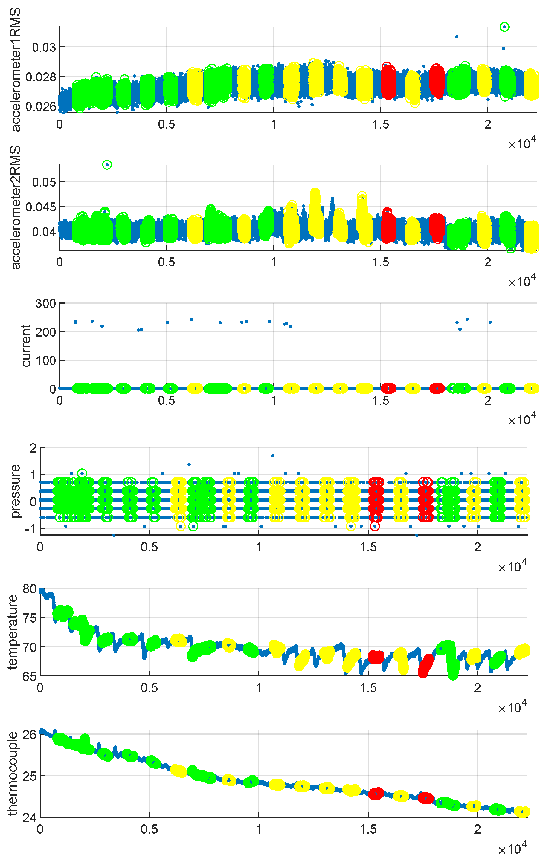
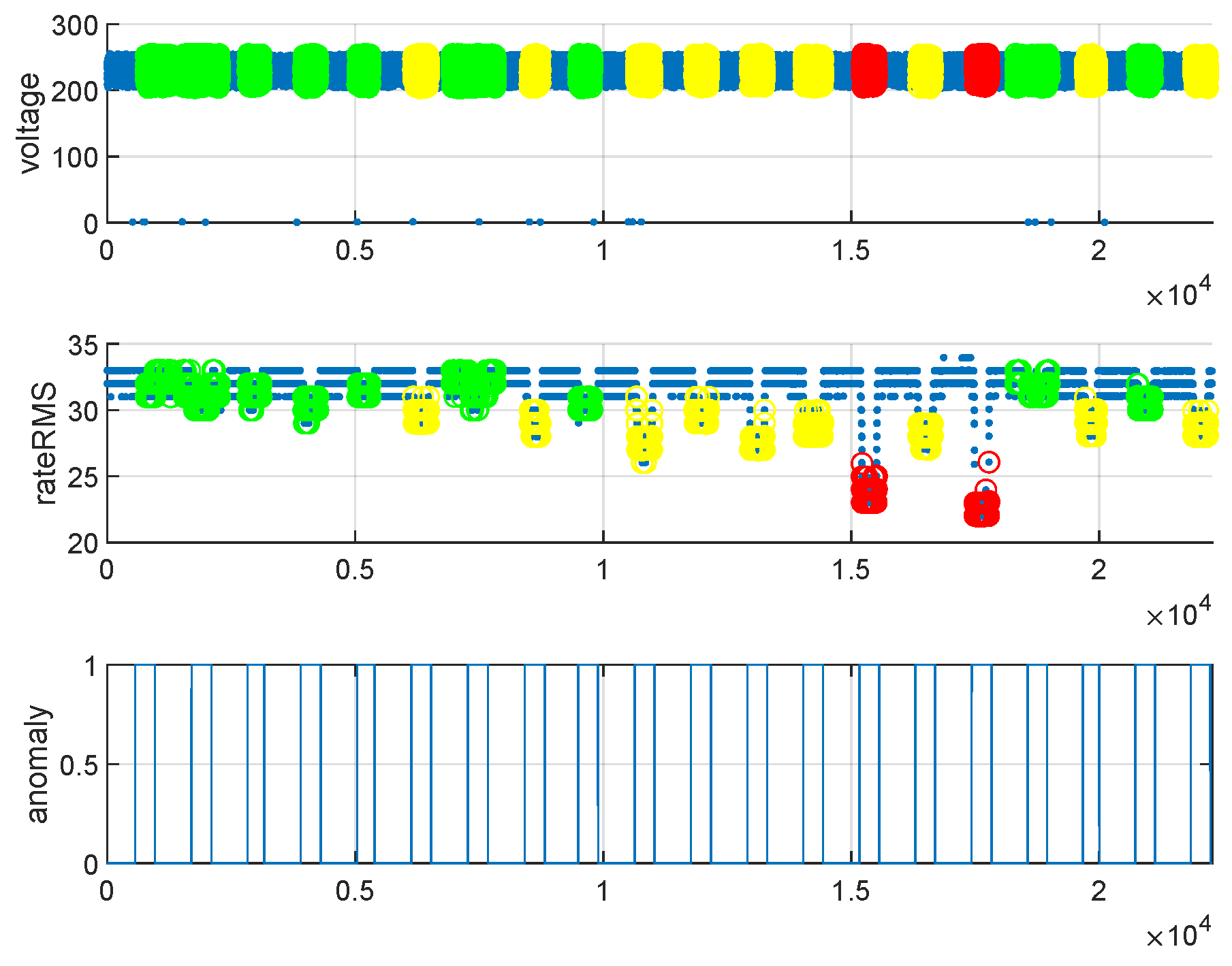
.
Figure 11 shows the results of anomaly detection and clustering on an excerpt of the SKAB data. According to the anomaly indicators in the bottom-right plot, all anomaly regions are correctly detected and clustered according to the severity (an increase from green to yellow to red). It is worth noting that the original datasets do not provide any additional information about the anomaly types. Therefore, our clustering is mainly based on the structures of detected anomalies, and the severity of anomalies depends on the distance between the detected sequence and the baseline.


