


Design of Adaptive Kalman Consensus Filters (a-KCF)

Department of Aerospace Information and Control, School of Aeronautics and Astronautics, Shanghai Jiao Tong University, Shanghai 200240, China
*
Authors to whom correspondence should be addressed.
Signals 2023, 4(3), 617-629; https://doi.org/10.3390/signals4030033
Submission received: 17 May 2023
/
Revised: 30 July 2023
/
Accepted: 25 August 2023
/
Published: 31 August 2023
(This article belongs to the Special Issue Wireless Communications and Signals)
Abstract
:This paper addresses the problem of designing an adaptive Kalman consensus filter (a-KCF) which embedded in multiple mobile agents that are distributed in a 2D domain. The role of such filters is to provide adaptive estimation of the states of a dynamic linear system through communication over a wireless sensor network. It is assumed that each sensing device (embedded in each agent) provides partial state measurements and transmits the information to its instant neighbors in the communication topology. An adaptive consensus algorithm is then adopted to enforce the agreement on the state estimates among all connected agents. The basis of a-KCF design is derived from the classic Kalman filtering theorem; the adaptation of the consensus gain for each local filter in the disagreement terms improves the convergence of the associated difference between the estimation and the actual states of the dynamic linear system, reducing it to zero with appropriate norms. Simulation results testing the performance of a-KCF confirm the validation of our design.
1. Introduction
The problem of distributed estimation for linear dynamic systems via the cooperation and coordination of multiple fixed/mobile agents has been extensively explored by numerous researchers [1,2,3,4,5]. Distributed Kalman filtering has been broadly utilized as a powerful and efficient tool to solve the aforementioned scenario [1,6,7,8,9,10]. An essential problem involving cooperation of multi-agent systems that has attracted much attention is the consensus problem. In order to reconstruct the states of the dynamic system, a network of sensing agents is adopted; these may form either a homogeneous or a heterogeneous network. Each agent transmits state estimates to its immediate neighbors based on the communication topology. Through the consensus strategy, all agents in use eventually agree with each other on a common estimation value regarding the states of the dynamic system.
The early formal study of consensus problems [11] formed the basis of distributed computing [12], which has found wide and popular utilization in sensor network applications [13,14]. The dynamic consensus problem appears frequently in the cooperation and coordination of multi-agent systems, including scenarios such as formation control [5,9,15], self-alignment, flocking [4,16], and distributed filtering [1,17]. The typical consensus protocol and its performance analysis were first introduced by Olfati-Saber and Murray in the continuous-time model (see [3,7]). In [7], the authors considered a cluster of first-order integrators working cooperatively under the average consensus control algorithm, in which each agent finally agrees on a common value that is the average of initial states of all agents as the individual ultimate state. In [1], a distributed Kalman filtering (DKF) algorithm was proposed in which data fusion was achieved through dynamic consensus protocols [18]. Later, in [17], the same author extended the results of [1] to use two identical consensus filters for sensor fusion with different observation matrices, then presented [1] an alternative distributed Kalman filtering algorithm which applies consensus to the state estimates. This idea forms the foundation of the present paper, in which we propose an adaptive Kalman consensus filtering algorithm. In [9], the authors presented a different view towards designing consensus protocols based on the Kalman filter structure. By adjusting the time-varying consensus gains, [9] proved that consensus can be achieved asymptotically under a no-noise condition. In addition, graph theory [7,19,20] has been adopted to construct the communication topology among distributed agents. In this paper, we assume a fixed topology; however, it is not necessarily relaxed to the point of all-to-all connection. This means that each agent is not constrained in communication with others, a consideration that would be more practical in real-world applications.
Recently, many extensions of consensus protocols have been explored to improve the convergence rate of dynamic systems among cooperative agents. This includes the study of communication topology design [21,22], optimal consensus-based estimation algorithms [2,23,24], and adaptive consensus algorithms [25,26,27] in both continuous-time and discrete-time scenarios. Other extensions for system control purposes have been studied to realize finite time consensus among agents, methods of which involves event-triggered and sliding mode control [28,29]. These research fruits have been considered and embedded in Kalman filtering algorithms [30,31], although the complexity of the algorithms makes practical implementation challenging, particularly when compared to the adaptive weight parameter method proposed in this paper.
The main contribution of this paper is to derive an adaptive Kalman consensus filtering (a-KCF) strategy in a continuous-time model and analyze its stability and convergence properties. Extensive simulation results aim to demonstrate better effectiveness of a-KCF compared with the previous work of Olfati-Saber[17] along with a faster convergence rate of the estimation error when the consensus gains change adaptively based on the disagreement of these filters.
The remainder of this paper is organized as follows. In Section 2, we provide preliminaries on algebraic graph theory [20], which is the basis of the consensus strategy. In Section 3, we provide a retrospective view of the previous work of Olfati-Saber on the Kalman consensus filtering algorithm, which our analysis relies upon. In Section 4, we illustrate the main results of this paper, namely, derivation of the adaptive Kalman consensus filtering algorithm. The purpose is to adaptively adjust the consensus gain as the weight applied to the disagreement terms in order to improve the convergence of the estimation error. Simulation results are presented in Section 5, then we conclude our work in Section 6.
The following notations are be used throughout this paper: and denote the n dimensional square matrices and the set of all matrices, respectively. denotes the identity matrix with dimension . For a given vector or matrix, represents the transpose of the matrix A. For a given square matrix A, denotes its trace and the norm of A is defined by . If , this indicates a random variable f that complies with a Gaussian distribution with mean a and variance .
2. Problem Statement
Consider a continuous-time dynamic system that has the following form:
with m states measured by n distributed agents via sensing devices and local filters. Here, denotes the states of this dynamic system, represents the dynamical matrix, represents the white Gaussian noise of the system, which is distributed by the matrix B with zero mean and covariance , is the initial guess for the states of the dynamic system with error covariance , and the sensing capability of each agent is determined by the following equation:
with the measurement matrix . The sensing devices are not able to measure all the states of the system; thus, only partial information is available to the local filters for the state estimation. Here, represents the white Gaussian noise of measurement for the ith agent, with zero mean and covariance matrix . Throughout this paper, we assume that there is no noise coupling effect among the agents; therefore, we can set both and as diagonal matrices. The main purpose of this paper is to design an adaptive state estimation structure for each agent such that the state estimation of individuals can be exchanged among their immediate neighbors through the communication topology .
2.1. Graph Theory Preliminaries
We consider n distributed agents working cooperatively through a communication network/topology characterized by a weighted graph with inconsistent information, where represents the set of agents, denotes the set of edges in , and represents the connected bridge of an ordered pair . For each , we mean that the ith agent can only receive information from the jth agent, not vice versa. In such cases, we call j the neighbor of i and denote as the set of neighbors of the ith agent. If , this means that there is no communication link between the jth and ith agents.
Let represent the adjacency matrix of , defined as and ; otherwise, .
We define the in-degree of the ith agent as and the out-degree of the ith agent as ; then, the graph Laplacian of can be defined as , where .
One important property of L (see [19] for more details) is that all eigenvalues of L are non-negative, and at least one of them is zero. If we denote as the ith eigenvalue of L, then we have the following valid relation for any graph : [32].
In a special case, if the in-degree of the ith agent or , then we call the graph , as an all-to-all connected topology. In such cases, the graph Laplacian L is a symmetric and positive-semidefinite matrix with only one zero eigenvalue.
2.2. Consensus Protocols
Several types of consensus protocols have been explored, and these have been utilized in many different scenarios over the years. In this paper, we mainly adopt the “consensus in network” strategy mentioned in [17].
Using the background information provided in Section 2.1 and assuming that there are n integrator agents working cooperatively with dynamics , the “consensus in network” strategy forces those agents to reach an agreement on their states by .
This distributed dynamic structure demonstrates that the ith agent updates its state by penalizing the state disagreement between its immediate neighbor and itself in order to ensure that all of those n agents finally agree on a common value as their ultimate state. Via this protocol, which [17] proved to be stable and convergent, we can say consensus is achieved through the communication and cooperation among the agents.
Furthermore, we can explore the collective dynamics of individual agents in the graph , which can be expressed as , where L is the aforementioned graph Laplacian in Section 2.1.
3. Kalman Consensus Filtering Algorithm
In this section, we provide a retrospective view of the previous work of Olfati-Saber [17], in which the author presented the continuous-time distributed Kalman filtering strategy without adopting the consensus filtering algorithm, instead forcing consensus through state estimates. We treat this work as the fundamental background for designing our adaptive Kalman consensus filters.
In [17], the author considered n distributed agents working cooperatively to complete a common task for estimating the state of a linear system, defined in Equation (1), with the sensing capability defined as in Equation (2). Each agent shares its instant state estimates with its immediate neighbors through the communication topology . Olfati-Saber [17] proposed individual agents applying the following distributed estimation algorithm:
with initial conditions and .
Through this distributed algorithm, it was claimed that the collective dynamics of the estimation errors are (in the absence of noise, this assumption is made to ease the computation complexity of the proof; later work showed that even if process and measurement noise are present, the stability and convergence properties of the adaptive Kalman consensus filtering algorithm remain valid). The errors converge to zero through analysis of the Lyapunov function . Furthermore, all agents with the estimator structure in Equation (3) asymptotically agree with each other on their state estimates, which match the value of the true states of the linear system in Equation (1), such as . See the proof in [17] for more detail.
4. Adaptive Kalman Consensus Filtering
In this section, we show our main contribution to this paper, in which we consider adding an adaptation mechanism to the Kalman consensus filtering algorithm shown in Section 3. We name this adaptive Kalman consensus filtering, or a-KCF. The proposed ith agent estimation structure with adaptive gain on the consensus term is as follows:
where represents the state estimates of the ith agent and is the scalar adaptive gain of the estimation differences between the ith agent and its neighbors. The consensus weighting matrix is designed based on Lyapunov stability analysis, as detailed in the following part.
If we consider a scenario in which no noise affects the error dynamics, as proposed in [17], in a similar fashion, we can derive the local error dynamic of the ith agent using the fact that , as shown below:
The basic idea for seeking the adaptive gain involves consideration of two aspects:
- The proposed adaptive Kalman consensus filter has stable performance.
- The associated error dynamic asymptotically converges to zero.
Lemma 1.
The proposed distributed estimator structure of the ith agent with adaptive gains for each disagreement term is provided by Equation (4). By means of analyzing a Lyapunov function , where is a symmetric positive definite matrix, the local adaptation law can be derived by satisfying the system stability conditions for both and , which turns out to be .
Proof.
We consider the following local Lyapunov function for the ith agent based on Lyapunov redesign methods
where is a symmetric positive definite solution of the following Lyapunov equation:
with the assumption that is a symmetric positive definite matrix and all eigenvalues of the matrix have negative real parts.
Because , there exist many ways to design in order to satisfy the aforementioned assumption. One possible way is to use the pole placement method to design the value for such that generates an exponentially stable local system.
Now, the derivative of is provided by . By substituting from Equation (5) into Equation (6), we obtain the following expression:
In order to further simplify Equation (8), we can assume the weighted consensus matrix . Thus, the expression of is
Therefore, by setting the sum of the last two terms in Equation (9) to equal zero, we can derive the adaptation law shown below:
Therefore, the local adaptation law is now provided by
□
Remark 1.
The choice of the structure of is not necessarily unique; it is only necessary for it to be possible to cancel out the term in Equation (8), along with the arbitrary matrix , which has an appropriate dimension such that and are available signals for the estimation process. Here, we choose for simplification.
Furthermore, if we examine the derivative of , then we find that
However, we can only argue that
This means we need additional arguments to guarantee that the convergence of reaches zero, as is only negative semi-definite. Thus, in order to show that each individual error dynamic asymptotically converges to zero, we need to examine the collective error dynamics for all agents.
Let us denote as the collective error vector; now, we can write the collective error dynamics in the following form (without noise):
where and
Remark 2.
The row sum of Γ is zero; furthermore, the sum of the off-diagonal entries in each row is equal to the negative value of the corresponding diagonal entry. The operator ⊗ denotes the Kronecker product, while denotes a identity matrix.
Theorem 1.
Consider a wireless sensor network consisting of n agents which form a communication topology . Each agent adaptively estimates the states of a linear dynamic system with the structure governed by Equation (4) using the local adaptation law in Equation (11). Each satisfies the Lyapunov equation as in Equation (7). Then, the collective dynamics of the estimation errors in Equation (14) (without noise) represent a stable system. Furthermore, the adaptive Kalman consensus filter (a-KCF) and the adaptation law law can be implemented through Algorithm 1, which generates a stable estimation system.
Proof.
We now can write the collective Lyapunov function as follows:
We denote , where each entry in is a symmetric positive definite solution of Equation (7) with respect to a different index i.
Then, we take the derivative of V and combine it with the adaptation law in Equation (11), resulting in the following expression:
where and each entry of must satisfy Equation (7) for the corresponding ith index.
Therefore, we can argue that the collective error dynamics and from Equation (20) are bounded; thus, we can say that . From Equation (16), it can be concluded that is bounded as well, that is, . Therefore, using Barbalat’s Lemma, we can write as ; in other words, the error dynamics of each agent asymptotically converge to zero. □
| Algorithm 1 Adaptive Kalman Consensus Filter |
|
Special case: when the adaptive gain
If we assume that the adaptive gains for all neighbors of the ith agent are identical, such that . Then, we can take the term out of the summation in Equation (4); in this manner, we can further simplify the structure of in Equation (15) to . Therefore, the error dynamics in Equation (16) change to
where L is the graph Laplacian of the communication topology .
Therefore, we can rewrite the adaptation law in this special case as follows:
Remark 3.
By carefully examining the above analysis, we find that there is vagueness when observing the agreement evolution of our adaptive Kalman consensus filters. Thus, it is necessary to show that the convergence of individual a-KCF to a common value, which implies that each agent agrees with the others on their estimates. To this end, it is necessary to define a quantity to measure the disagreement level of the proposed a-KCF.
Lemma 2.
In a similar manner as [17], we define the measure of disagreement of n a-KCFs as follows:
where is the mean estimate of n a-KCFs. Therefore, represents the deviation of each agent’s estimate from the mean estimate. Furthermore, by examining the disagreement dynamics of Equation (23), it is proved to converge to zero in finite time.
Proof.
The measurement of disagreement can be transformed into the following expression:
Then, we can write the collective dynamics of as follows:
It can instantly be recognized that the convergence of is related to the convergence of . We have proved that converges to zero in finite time; however, due to the zero eigenvalue of the matrix , Equation (24) does not simply imply that converges to zero in finite time. Therefore, we need to find an alternate approach to prove this lemma.
Let us define as the estimate difference between the ith and the jth agents and denote as the estimation error difference between the ith and the jth agents. It is immediately clear that . Now, we can rewrite Equation (23) into the following form:
From Equation (26), it can be argued that if we are able to prove the convergence of the dynamics of or to zero in finite time, we can conclude that converges to zero, as .
For simplification, consider the special case when . According to Equation (5), we can find the dynamics of as follows:
In Section 4, we showed that generates an exponentially stable linear dynamic system for the ith agent, while both and , along with , are bounded quantities. In the proof of Theorem 1, we concluded that ; hence, . To complete this proof, we need to prove that both and are bounded.
We now proceed to study the norm of , which is denoted as ; then,
From above, it can be proved that ; therefore, we can conclude that converges to zero, as . Furthermore, in Equation (26) converges to zero in finite time. □
5. An Example
Consider a linear dynamic system in Equation (1) with ; assume that there are three agents distributed in a 2D domain. Each agent embeds a sensing device with measurement capability , such as .
It is clear while that the system itself is not observable by individual agents, it is observable through all of them. In this simulation, we carry out a comparison between the Kalman consensus filtering algorithm proposed by Olfati-Saber in [17] and our adaptive Kalman consensus filtering algorithm from Theorem 1 on their performance and effectiveness.
We set up our simulation with the following parameter configuration:
- Kalman Consensus FilterThe process noise distribution matrix is , and the covariance matrix of the process noise and measurement noise are and , respectively. We assume the initial conditions for the error covariance matrices of the agents to beWe set the initial value of as 1. Furthermore, we assume that each agent can receive and transmit its own information to the other two; we call this type of communication a full-connectivity topology. Therefore, the associated graph Laplacian has the following expression:
- Adaptive Kalman Consensus Filter
In both cases above, we assume the same initial conditions for the error dynamics, such as ; and . In order to construct a fair comparison between the KCF and a-KCF algorithms, we assume that the dynamics of the error covariance matrix in Equation (3) comply with the algebraic Riccati equation, and use the same filter gains in both cases.
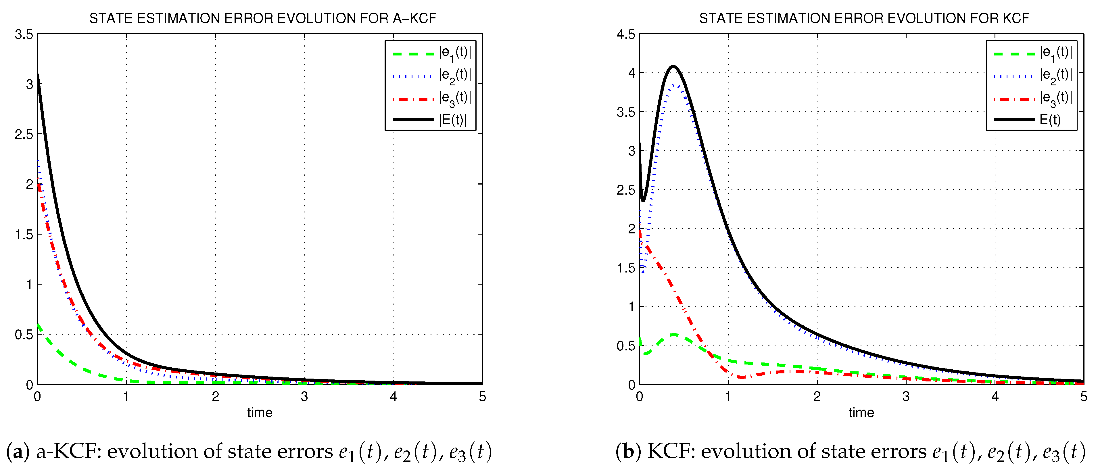
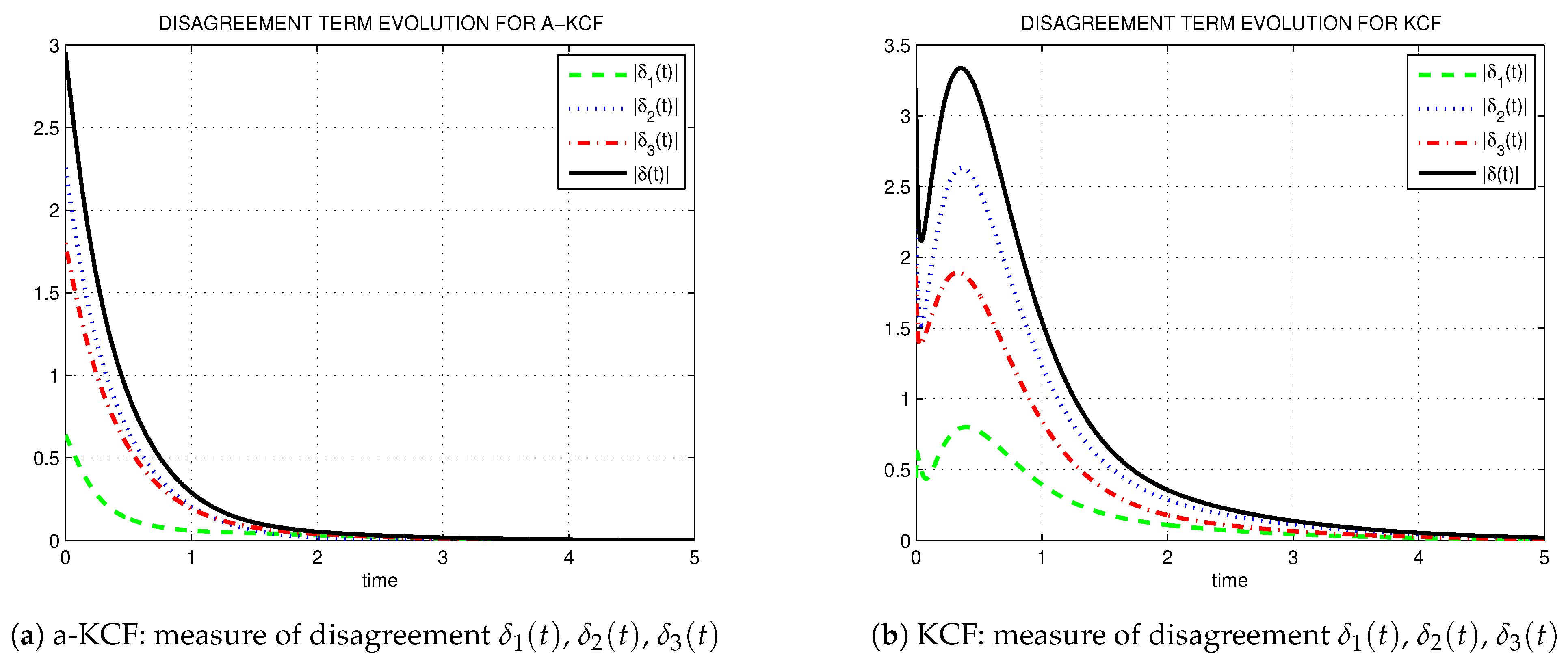
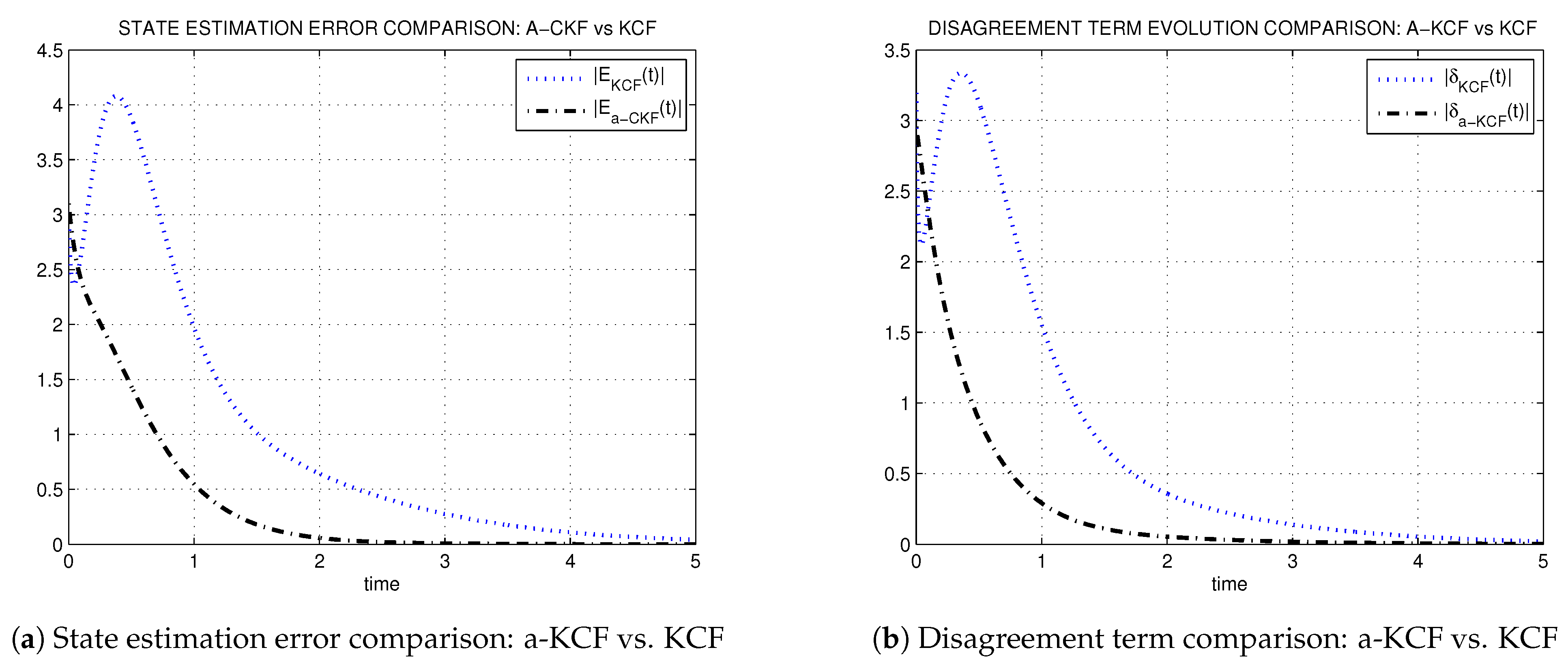
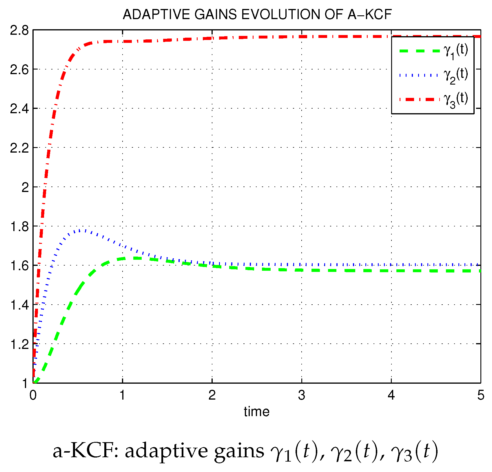
The simulation results are shown in Figure 1, Figure 2, Figure 3 and Figure 4. From a comparison of Figure 1a,b, we can conclude that a-KCF has better performance regarding the error convergence rate than the KCF in [17]. Figure 2a,b illustrates the evolution of the disagreement term in both the KCF and the a-KCF algorithms. According to the simulation results in Figure 3a,b, both the state estimation error and the disagreement term converge faster in the a-KCF case. Figure 4 demonstrates the dynamics of the adaptive gain.
6. Conclusions
In this paper, the problem of n distributed agents working cooperatively through a communication network to estimate the true state of a linear dynamic system has been considered for both the non-adaptive DKF algorithm proposed by Olfati-Saber [17] and our proposed adaptive Kalman consensus filtering (a-KCF) algorithm. Stability and performance analyses are demonstrated for the a-KCF algorithm, showing that our adaptive extension of Olfati-Saber’s work in [17] has better convergence performance for the collective dynamics of the estimation errors. The simulation results in Section 5 match our theoretical analysis. Moreover, the a-KCF algorithm turns out to be a suboptimal one which neglects the coupling effect among the agents’ cooperation. For simplification, we only consider the no-noise scenario. However, we recognize the benefit of the a-KCF algorithm in that it lowers the communication complexity from to and has better scalability when more agents join the network.
Author Contributions
S.Y. was responsible for the conceptualization of the research study, carried out the formal analysis, and contributed to the original draft of the manuscript. He also conducted the simulation experiments and took the lead in the final writing of the paper. S.W. guided the direction of research through the development of the methodology and was responsible for the validation of the analysis and simulation results. Additionally, S.W. secured the funding for the project and oversaw its administration. All authors have read and agreed to the published version of the manuscript.
Funding
This research was funded by National Natural Science Foundation of China OF FUNDER grant number U20B2054.
Data Availability Statement
All data generated or analyzed during this study are included in this published article.
Conflicts of Interest
The funders had no role in the design of the study; in the collection, analyses, or interpretation of data; in the writing of the manuscript, or in the decision to publish the results.
References
- Olfati-Saber, R. Distributed Kalman filter with embedded consensus filters. In Proceedings of the 44th IEEE Conference on Decision and Control, Seville, Spain, 12–15 December 2005; pp. 6698–6703. [Google Scholar]
- Olfati-Saber, R. Kalman-Consensus Filter: Optimality, Stability, and Performance. In Proceedings of the 48th IEEE Conference on Decision and Control and 28th Chinese Control Conference, Shanghai, China, 16–18 December 2009; pp. 7036–7042. [Google Scholar]
- Olfati-Saber, R.; Shamma, J.S. Consensus filters for sensor networks and distributed sensor fusion. In Proceedings of the 44th IEEE Conference on Decision and Control, Seville, Spain, 12–15 December 2005; pp. 6698–6703. [Google Scholar]
- Olfati-Saber, R. Flocking for multi-agent dynamic systems: Theory and algorithms. IEEE Trans. Autom. Control 2006, 51, 401–420. [Google Scholar] [CrossRef]
- Olfati-Saber, R.; Murray, R.M. Agreement problems in networks with directed graphs and switching topology. In Proceedings of the 42nd IEEE Conference on Decision and Control, Maui, HI, USA, 9–12 December 2003; pp. 4126–4132. [Google Scholar]
- Olfati-Saber, R.; Fax, J.A.; Murray, R. Consensus and cooperation in networked multi-agent systems. In Proceedings of the 46th IEEE Conference on Decision and Control, New Orleans, LA, USA, 12–14 December 2007; pp. 215–233. [Google Scholar]
- Olfati-Saber, R.; Murray, R.M. Consensus problem in networks of agents with switching topology and time-delays. IEEE Trans. Autom. Control 2004, 49, 1520–1533. [Google Scholar] [CrossRef]
- Xiao, F.; Wang, L.; Jia, Y. Fast information sharing in networks of autonomous agents. In Proceedings of the 2008 American Control Conf, Seattle, WA, USA, 11–13 June 2008; pp. 4388–4393. [Google Scholar]
- Ren, W.; Beard, R.W.; Kingston, D.B. Multi-agent Kalman consensus with relative uncertainty. In Proceedings of the 2005 American Control Conference, Portland, OR, USA, 8–10 June 2005; pp. 1865–1870. [Google Scholar]
- Crassidis, J.L.; Junkins, J.L. Optimal Estimation of Dynamic Systems; Applied Mathematics and Nonliear Science Series; Chapman & Hall: Boca Raton, FL, USA, 2004. [Google Scholar]
- DeGroot, M.H. Reaching a Consensus. J. Appl. Probab. Available online: https://pages.ucsd.edu/~aronatas/project/academic/degroot%20consensus.pdf (accessed on 30 July 2023).
- Lynch, N.A. Distributed Algorithms; Morgan Kauffman: Burlington, MA, USA, 1997. [Google Scholar]
- Ren, W.; Beard, R.W. Consensus seeking in multiagent systems under dynamically changing interaction topologies. IEEE Trans. Autom. Control 2005, 50, 655–661. [Google Scholar] [CrossRef]
- Ren, W.; Beard, R.W.; Atkins, E.M. A survey of consensus problems in multi-agent coordination. In Proceedings of the 2005 American Control Conf, Portland, OR, USA, 8–10 June 2005; pp. 1859–1864. [Google Scholar]
- Carli, R.; Chiuso, A.; Schenato, L.; Zampieri, S. Distributed Kalman filtering based on consensus strategies. IEEE J. Sel. Areas Commun. 2008, 26, 622–633. [Google Scholar] [CrossRef]
- Jadbabaie, A.; Lin, J.; Morse, A.S. Coordination of groups of mobile autonomous agents using nearest neighbor rules. IEEE Trans. Autom. Control 2003, 48, 988–1001. [Google Scholar] [CrossRef]
- Olfati-Saber, R. Distributed Kalman filter for sensor networks. In Proceedings of the 46th IEEE Conference on Decision and Control, New Orleans, LA, USA, 12–14 December 2007; pp. 5492–5498. [Google Scholar]
- Olfati-Saber, R.; Murray, R. Consensus protocols for networks of dynamic agents. In Proceedings of the 2003 American Control Conference, Denver, CO, USA, 4–6 June 2003; pp. 951–956. [Google Scholar]
- Godsil, C.; Roylea, G. Algebraic Graph Theory; Springer: New York, NY, USA, 2001. [Google Scholar]
- Ren, W.; Beard, R.W. Consensus of information under dynamically changing interaction topologies. In Proceedings of the 2004 American Control Conference, Boston, MA, USA, 10–12 June 2004; pp. 4939–4944. [Google Scholar]
- Cao, M.; Wu, C.W. Topology design for fast convergence of network consensus algorithms. In Proceedings of the IEEE International Symposium on Circuits and Systems, New Orleans, LA, USA, 27–30 May 2007; pp. 1029–1032. [Google Scholar]
- Zhou, J.; Wang, Q. Convergence speed in distributed consensus over dynamically switching random networks. J. Autom. 2009, 45, 1455–1461. [Google Scholar] [CrossRef]
- Yang, P.; Freeman, R.A.; Lynch, K.M. Optimal information propagation in sensor networks. In Proceedings of the 2006 IEEE International Conference on Robotics and Automation, Orlando, FL, USA, 15–19 May 2006; pp. 3122–3127. [Google Scholar]
- Hui, Q.; Zhang, H. Optimal linear iterations for distributed agreement. In Proceedings of the 2010 American Control Conference, Baltimore, MD, USA, 30 June–13 July 2010; pp. 81–86. [Google Scholar]
- Taleb, M.S.; Kefayati, M.; Khalaj, B.H.; Rabiee, H.R. Adaptive consensus averaging for information fusion over sensor networks. In Proceedings of the 2006 IEEE International Conference on Mobile Adhoc and Sensor System, Vancouver, BC, Canada, 9–12 October 2006; pp. 562–565. [Google Scholar]
- Wang, L.; Zhang, Q.; Zhu, H.; Shen, L. Adaptive consensus fusion estimation for MSN with communication delays and switching network topologies. In Proceedings of the 49th IEEE Conference on Decision and Control, Atlanta, GA, USA, 15–17 December 2010; pp. 2087–2092. [Google Scholar]
- Sumizaki, K.; Liu, L.; Hara, S. Adaptive consensus on a class of nonlinear multi-agent dynamical systems. In Proceedings of the SICE Annual Conference, Taipei, Taiwan, 18–21 August 2010; pp. 1141–1145. [Google Scholar]
- Li, Z.; Liu, Y.; Hu, X.; Dai, W. Event-triggered optimal Kalman consensus filter with upper bound of error covariance. J. Signal Process. 2021, 188, 108175. [Google Scholar] [CrossRef]
- Zuo, Z.; Han, Q.; Ning, B.; Ge, X.; Zhang, X. An overview of recent advances in fixed-time cooperative control of multiagent systems. IEEE Trans. Ind. Inf. 2018, 14, 2322–2334. [Google Scholar] [CrossRef]
- Li, W.; Jia, Y.; Du, J. Distributed Kalman consensus filter with intermittent observations. J. Frankl. Inst. 2015, 352, 3764–3781. [Google Scholar] [CrossRef]
- Liu, C.; Sun, S. Event-triggered optimal and suboptimal distributed Kalman consensus filters for sensor networks. J. Frankl. Inst. 2021, 358, 5163–5183. [Google Scholar] [CrossRef]
- Olfati-Saber, R. Algebraic connectivity ratio of Ramanujan graphs. In Proceedings of the 2007 American Control Conference, New York, NY, USA, 9–13 July 2007; pp. 4619–4624. [Google Scholar]
Figure 1.
Evolution of state errors vs. time.

Figure 2.
Evolution of disagreement term vs. time.

Figure 3.
Performance comparison examining state estimation error and disagreement term evolution vs. time.
Figure 3.
Performance comparison examining state estimation error and disagreement term evolution vs. time.

Figure 4.
Adaptive gains evolution vs. time.

Disclaimer/Publisher’s Note: The statements, opinions and data contained in all publications are solely those of the individual author(s) and contributor(s) and not of MDPI and/or the editor(s). MDPI and/or the editor(s) disclaim responsibility for any injury to people or property resulting from any ideas, methods, instructions or products referred to in the content. |
© 2023 by the authors. Licensee MDPI, Basel, Switzerland. This article is an open access article distributed under the terms and conditions of the Creative Commons Attribution (CC BY) license (https://creativecommons.org/licenses/by/4.0/).
Share and Cite
MDPI and ACS Style
Ye, S.; Wu, S. Design of Adaptive Kalman Consensus Filters (a-KCF). Signals 2023, 4, 617-629. https://doi.org/10.3390/signals4030033
AMA Style
Ye S, Wu S. Design of Adaptive Kalman Consensus Filters (a-KCF). Signals. 2023; 4(3):617-629. https://doi.org/10.3390/signals4030033
Chicago/Turabian StyleYe, Shalin, and Shufan Wu. 2023. "Design of Adaptive Kalman Consensus Filters (a-KCF)" Signals 4, no. 3: 617-629. https://doi.org/10.3390/signals4030033