Article

DXN: Dynamic AI-Based Analysis and Optimisation of IoT Networks’ Connectivity and Sensor Nodes’ Performance

School of Computing, The University of Buckingham, Buckingham MK18 1EG, UK
*
Authors to whom correspondence should be addressed.
Signals 2021, 2(3), 570-585; https://doi.org/10.3390/signals2030035
Submission received: 14 May 2021 / Revised: 9 August 2021 / Accepted: 31 August 2021 / Published: 3 September 2021
(This article belongs to the Special Issue Wireless Communications and Signals)

Abstract

:
Most IoT networks implement one-way messages from the sensor nodes to the “application host server” via a gateway. Messages from any sensor node in the network are sent when its sensor is triggered or at regular intervals as dictated by the application, such as a Smart-City deployment of LoRaWAN traps/sensors for rat detection. However, these traps can, due to the nature of this application, be moved out of signal range from their original location, or obstructed by objects, resulting in under 69% of the messages reaching the gateway. Therefore, applications of this type would benefit from control messages from the “application host server” back to the sensor nodes for enhancing their performance/connectivity. This paper has implemented a cloud-based AI engine, as part of the “application host server”, that dynamically analyses all received messages from the sensor nodes and exchanges data/enhancement back and forth with them, when necessary. Hundreds of sensor nodes in various blocked/obstructed IoT network connectivity scenarios are used to test our DXN solution. We achieved 100% reporting success if access to any blocked sensor node was possible via a neighbouring node. DXN is based on DNN and Time Series models.

Graphical Abstract

1. Introduction

Artificial Intelligence (AI) provides the ability to make decisions without the interaction of humans which makes it attractive for “network traffic monitoring and management”. AI engines are used for IoT applications for predicting, amongst others, the changes in the collected application data (e.g., temperature and humidity readings). Another use is for predicting the behaviour of the IoT Sensor Nodes (SN) (e.g., signal strength and power levels). Therefore, AI can be the best QoS tool for IoT networks by forcing certain SNs to behave in a certain way to mitigate certain networking issues (e.g., re-routing) [1].
Deployment of some LPWAN (Low Power WAN) technologies such as LoRaWAN (Long Range WAN) demonstrates that there are real-time implementational issues, depending on the application and the SN deployment method, such as: (1) limited connectivity time for any one SN as more and more SNs added to the network due to the duty-cycle restriction [2], (2) SN signals can be blocked by obstacles especially for indoor connectivity scenarios [3], and (3) SNs can be moved around to a different location where it becomes out of range of the Gateway (GW) [4]. Feedback from actual deployments, such as the rat trap application example mentioned earlier, reveals some serious issues of this nature that need intelligent addressing.
Therefore, we believe that IoT networks would greatly benefit from an AI controller that studies all the received messages data of the network to mitigate/overcome these challenges in real-time. For the above three issues, the AI controller can put some non-active SNs to sleep to ease the duty-cycle restriction. Moreover, to overcome the “out of range” issue (i.e., an SN becomes too far away from the gateway) and/or when an “obstacle presents itself in the SN signal path”, the AI system can mitigate these issues by arranging for a neighbouring SN to temporarily act as a bridge node for reaching the blocked SN message to the GW. Furthermore, this AI controller will make sure, independent of human help, that the nodes carrying out the bridging will maintain connectivity without running out battery power and that load-balance with other neighbouring SNs is achieved before the situation is rectified.
The proposed DXN AI-based engine detailed in this paper performs real-time analysis/monitoring of the collected data from all messages of the network and then make live decisions to change the behaviour of certain SNs as necessary to overcome any of the connectivity issues noted above.
The remaining of the paper is organised as follows: Section 2 summarises the most recent literature that we have chosen to review here; Section 3 details the DXN implementation with the test case scenarios/experiments and the obtained results; and finally, this work is concluded in Section 4.

2. Literature Review

The current expansion of the IoT SN devices and the communication technologies to support them necessitates the emergence of more scalable IoT networks. Current IoT networks/applications are limited because the “things”/SN devices have to be low-power and cheap. Moreover, the LPWAN technologies suffer from a limited data bandwidth due to duty cycle restrictions. Furthermore, most IoT networks are deployed as a star network (in a one-way communication). This is limiting, in that they lack the feedback mechanism that is used for application data purposes and can be used for enhancing the networking QoS.
We found that the literature contains attempts of researchers in LPWAN to improve IoT networks by inserting relay/repeater nodes in the network to improve their connectivity. Much of the literature focuses on the limitations of the LPWAN in general and LoRaWAN in particular. When in some deployment scenarios, certain SNs fall out of the GW’s reach due to reasons such as communication range and/or signal blockage due to obstacles or interference. The following is of a subset of the papers that we reviewed which have contributed to the design of our DXN solution.
Utilising the communication between the SNs and the host server was addressed by proposing a clustering technique for Machine-to-Machine (M2M) devices in an IoT network [5]. The technique was based on forming the clusters and selecting the Cluster Heads (CH) based on three factors: the node’s energy availability, interest ties (the relation strength between the M2M devices), and physical ties (the physical proximity and the communication link quality of the M2M devices). Once the cluster and the CH are formed and selected, these factors and sensor readings will be transmitted to the network host server via the CH. The host server (User) can use this information to make new decisions if necessary. This idea is similar to our DXN solution in the sense of creating a two-way relationship between the network and the host server where the collected information can be used to generate feedback to the network.
Proposing a relay mechanism is not something new; many proposals [6] have suggested using special devices such as repeaters (mostly are mains powered) in a fixed architecture deployment scenario. Others suggest deploying extra GWs. This makes it challenging to implement such solutions efficiently using regular LoRa SNs (small battery-powered expected to last for many years). Because these SNs have limited resources, there is no synchronisation between them, and they are sending/receiving at different times using different channels that are selected randomly. However, there was an attempt to facilitate a regular relay node dedicated to helping other SNs (end SNs) that are struggling to reach the GW [7]. These relay SNs are responsible for synchronising and forwarding messages from end SNs when they fail to reach the GW directly. To achieve this, two channels will be defined for every SN in the network. The relay SNs will be scanning these two channels every 500 ms separately. Before an end SN sends its packet, it will send a “wake-up sequence” (WS) message transmitted in an implicit header mode (no PHY header to minimise the overhead) on one of these channels. The WS message includes the randomly selected channel and data rate that the end SN will be using for the upcoming packet transmission, plus the time of the transmission. Once this WS message is received by a relay node, it can go back to sleep mode and later wakes up to the right channel/data rate just before the arrival of the end SN packet. When that packet arrives, the relay SN will acknowledge it first and then will encapsulate and forward it to the GW. The end SN will go back to sleep mode as well and open a receive window after 17 s to receive the acknowledgement (Ack) from the GW through the relay SN. The authors claim that the relay SN’s Ack message will include timing correction information to sync the end SN clock. This proposed method claims that with the relay SN sensing the two channels every 500 milliseconds, then the battery capacity for 5 years of operation will be 2.88 Amp.hour (A.h). Furthermore, for an end SN that transmit every 30 min, the battery capacity will be 0.16 A.h, which can be reduced to 0.08 A.h in case it transmits every 6 h. Although the method is based on using relay SNs with regular resources just as a typical LoRa SN, it is still fully dependent on these dedicated relay SN devices. That means that these relay SNs need to be strategically deployed in order to be useful. Therefore, it is less suitable for dynamic SN deployments, or the environment of the application changes the SN positions. Furthermore, this method suggests dedicating two channels for the handshake, and once these channels are used, they will be unavailable to use again for a certain amount of time, due to the duty cycle restrictions. Therefore, in the case of more than two end SNs available, they will be unable to use these channels. However, this work has inspired us to focus on enhancing regular SNs that can be adjusted as needed, on the go, to perform the bridging instead of a dedicated relay SN.
The first inspiration for DXN came from an AI-based project to enhance the security of IoT devices against malware attacks [8]. This is because SNs are very vulnerable to all forms of breach as, by design, they are simple with minimum resources and so include minimum protection in pursuit of maximum battery life. This paper proposes a scheme that continuously analyses the information received from the IoT network SNs. The AI engine tries to detect anomalies in the SN’s code behaviour in comparison with its neighbouring SNs, in case the SN’s code has been tampered with by a hacker. This AI engine is based on a CNN model and is located at the host server in the cloud. This scheme claims to work irrespective of the connectivity technology/protocol of the IoT network. This scheme is achieved by first inserting debugging code, which runs on the assembly language code, in each of the SNs in the network. This debugging code helps to identify the code flow of the received messages from these SNs. Once the messages are received at the server, the process will extract features from the received code of every SN, including features such as its memory used, network type, system calls, etc., into a CSV file. The process then converts these extracted SN features into vectors represented as unique images (similar to creating QR images that have embedded information to be interpreted by the reader). The process concludes by AI analysis by the ZFNet, a CNN based model [9], to determine if an attack has been carried out. Therefore, once the scheme detects a suspicious code from any SN, it will prevent the data from being used by the application, and so prevent an attack from taking place. This scheme is dynamic in terms of processing and analysing the data received from the SNs continuously in real time. Thus, it claims to achieve a malware detection accuracy of 99.28%. In addition, the use of an AI engine helped to identify not only the attacks that have been trained with but also identifying new evolving attacks. This has inspired us to think about implementing an AI engine based in the cloud to conduct a continuous live analysis of the IoT network messages for our solution.
In pursuit of reducing battery energy spent by SNs communicating localised messages about whatever they sensing to the GW of an IoT network, the following article has implemented a smart clustering algorithm that balances the connectivity load of the SNs [10]. This will keep the various SNs in the network alive longer as they proved in their testing. The authors have proposed a dynamic Cluster Head Sensor Node (CHSN) allocation based on the cluster network activity and traffic based on a set criterion. This means that no one CHSN will drain down its energy handling the communication for its cluster SNs. This has also improved the message slots allowance, eliminating any unnecessary communications within the cluster. The load balancing algorithm used for the clusters is considered as an improvement to the existing LEACH clustering algorithm [11] (a technique based on selecting new CHSN each round within the cluster based on their energy levels). This implementation categorises the SNs based on their energy level, location and neighbouring SNs. This information is obtained from the accumulated database (located in the cloud and updated by CHSNs each round) by a fuzzy logic-based controller (a model that has the ability to recognise, represent, and utilise data that is vague). The actual SN data collected by its CHSN include the SN’s identifier, location, remaining energy level, average distance to neighbours and distance to the GW. Therefore, their proposed controller will, for each of the clusters in the network, generate a queue of all the potential CHSNs in descending order from the most capable to the least. Based on that, a new CHSN will be selected, and in its turn, it will broadcast a join request to the rest of the SNs in its cluster. Finally, and based on the available clusters and their sizes, this controller will create a scheduling table for message transmission for all SNs in every cluster. This schedule is sent to all SNs and is designed to control the SNs random transmission, by syncing messages of any cluster’s SNs at specific time slots. Therefore, the CHSN and its associated SNs will have less wake-up time than before. The results of their test scenarios claim an improvement in the SNs’ battery lifetime of up to 200% when compared to other conventional clustering techniques (LEACH-PSO [12] and LEACH). This work has inspired us that clustering techniques are the way to go in our DXN. We believe that clustering coupled with an AI engine analysis would be a powerful implementation to reduce the unnecessary communication traffic and preserve the power consumption of SNs.
Another study of clustered networks was conducted and claimed that 60–80% of the total power consumption of the whole network is consumed by the CHSN nodes themselves [13]. This next work solves this issue. It is interesting to us because it uses two wireless connectivity technologies (LoRa and Zigbee) to cluster SNs before reaching the GW. This is mainly to increase the range of the IoT network coverage to a larger network as well as making its management scalable (and so to reduce CHSN power wasting). LoRa SNs are used to connect tail-end clusters of ZigBee SNs network to transmit their data to a remote GW using the long-range capability of LoRa. Furthermore, the authors deployed an AI model to help analyse the deployment to propose a better network control for the active/sleep periods of the LoRa SNs in the network. This AI engine predicts the fluctuation in the collected data to identify the periods when each SN needs to be active or sleep. Their proposed AI model was trained on a dataset generated by collecting data from various similar IoT networks. Using this dataset in an Interrupted Poisson Process (IPP) (a discrete probability distribution that calculates the probability of occurrence of a number of given events in a fixed period of time) will help in describing the traffic requirement for each SN (i.e., searching for the optimal transmission threshold and transmission rate). This information is indexed at the GW and then sent to each corresponding SN. Therefore, the GW will be able to adapt to any changes, for instance, if any SN’s packet generation rate decreases, then based on the IPP outputs, the GW needs to apply a smaller redundancy threshold to that SN to reduce the power consumption. The GW also holds records of the active periods for each SN, so to be analysed by a shallow (a single layer) Recurrent Neural Network (RNN) to predict the trend of that SN’s activity. This way, the GW will be able to adjust the sleeping/active strategy for each SN over time regardless of any sudden changes. Therefore, CHSNs will only be active at peak times. The paper quoted that, by using this model, LoRa SNs are saving one half of their energy compared to staying active all the time. This is an interesting approach that showed how AI-based network traffic analysis can impact battery power consumption which is very important for IoT devices. Therefore, this inspired us to include SNs’ activity in relation to the environment where each SN is placed in our clustering technique design.
A level of intelligence can be implemented onboard SNs that will lead to balancing the load on the supporting GW (in terms of the number of SNs connecting/transmitting data through a GW at any one point in time). In LoRa, the duty cycle function inside SNs allows a GW to accommodate thousands of SNs at the same time. Moreover, this capability of connecting lots of SNs to a GW can be achieved either randomly or fixed. However, when using different types of SNs (including different types of sensors or transmitting at different intervals), it can create an imbalance in the load at the supporting GW level (traffic issue rather than SN numbers). A Game Theory (GT)-based intelligent engine was proposed to be implemented onboard the SNs to help each SN to select suitable GW among multiple available GWs for relaying its messages [14]. This approach uses a reputation model (rating GWs based on the transmission rate and time). This is based on feedback from SNs to evaluate the connectivity between the SN and the network server for the used GW. This approach will determine how successful a GW is in relaying data between the connected SNs and the network host server. By using Bayesian Game (BG) strategy (a strategy where participating players (the SNs) do not have information about other participating players, but they depend on their beliefs to make a decision to maximise their rewards), SNs will estimate the time required for transmitting their uplinks with the used power transmission. Then, based on how good the GW performs against this time estimation, SNs will give feedback to the GW that will be reconsidered in the reputation model. The network server will keep/update a record of all the GWs’ reputations, and whenever it receives an uplink from any SN, it will reply to it with a reward. High rewards are given for SNs that use GWs with low reputation, and low rewards are given for SNs that use GWs with high reputation, so to balance the load among GWs to transmit their data through it. The goal of each SN is to collect as many rewards as possible while maintaining a good connection to the server. This will maintain a load balance across all the available GWs. This approach was compared with both random and fixed SNs allocation in terms of Packet Delivery Ratio (PDR) and Packet Delivery Delay (PDD). The results claim that the reputation scoring model has achieved best with a PDR of 98% and a PDD of 15%. We believe that it is useful to include a load balancing model in our DXN solution to prevent the load imbalance at any bridging SN available within the range of more than one blocked SN.
The following section describes the compound features of DXN that we have adopted to ensure it delivers performance enhancement most suited to IoT networks, focusing on LoRaWAN deployments.

3. Design, Implementation and Test of the DXN Engine
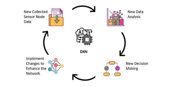
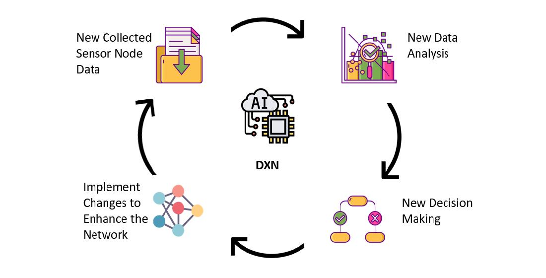
Since this project is focused on the wireless connectivity of sensor nodes in an LPWAN IoT networking, our original idea behind DXN is to introduce a dynamic SNs QoS management inside the host-server to feed the SNs with control messages to make new networking (connectivity/traffic/routing) decisions for the SNs’ messages. The implemented DXN is an AI-based engine that constantly collects data, analyses them, creates relations and statistics, forwards them to the network controller to then feedback control messages to SNs, and so on.

3.1. Why DXN

Note that some of the scenarios to the issues raised here are illustrated in detail in Section 3.4.1, Section 3.4.2 and Section 3.4.3.
Figure 1 shows a screenshot of SNs’ generated/sent data received by the host server in our deployed LoRaWAN IoT network (for example, the first column in the screenshot contains the SN address to communicate with the relevant SN, the second column contains the address of the end node in case the message is being forwarded, plus other information such as energy level to estimate its remaining battery life, RSSI, location, etc.). If these kinds of data are fed to an AI-based engine, there is potential to enhance the QoS of the network by continuously analysing the collected data. An AI engine will be able to make decisions that can be fed back to the SNs to adapt/change their behaviour according to the connectivity status of the network at that time. This will overcome certain networking QoS issues, such as:
  • When more than one middle/bridging SN is available nearby in the vicinity of an SN that is either blocked or out of GW reach, DXN will decide which of these middle/bridging SNs is used to forward through the messages of the blocked node. This will balance the connectivity amongst middle/bridging nodes without overusing certain bridging SNs more than others.
  • By analysing the transmission configurations used by each SN (for example, the used Spreading Factor (SF) or the used LoRaWAN frequency channel), DXN can change these configurations or update the frequency channels list for any SN that is affected by a harsh signal environment to prevent jitter or packet loss.
  • To maintain a healthy IoT network with minimum duty cycle restrictions, DXN can adjust the sleep/active times for each SN in the network based on its current transmission/relevance status, or the environment status. The rhythm of SN activity may change in some networks from time/environment to another, especially in agricultural applications, for example.
  • Furthermore, to point (3) above, by analysing the trend of the collected data, the activity of SNs could be predicted, and then “activity” will become an effective factor in SNs clustering for better network management, and load-balancing on any chosen middle/bridging node.
  • The AI engine productivity could be increased further by including simple extra information data within the SNs packets as inputs that will have a huge impact. However, including such extra information, data should be based on a considerate study to balance between the effort of the SNs and the improvement impact on the connectivity of the whole network. Examples of such data are:
    • Security, adding security details to help detecting/preventing certain attacks.
    • Priority, including priority details to help deciding the response/process time compared to others.
    • Type, including the SN type in the hybrid deployments, to help utilise each SN type efficiently.
    • Location, including location details to help make decisions that suit certain areas, such as deploying extra or fewer SNs.

3.2. The Problem Statement

We believe that to conduct any project implementation, it is best to have a real-time actual deployment to evaluate the results, and the implemented software and hardware features. For this project, we chose a partner company’s LoRaWAN IoT deployed network to solve two main issues they have: (1) range, where SNs might either be deployed out of the GW’s range, or maybe moved its position after the deployment, and (2) access, where any SN is unable to reach the GW due to its signal being obstructed by something (tall building/trees) or medium interference.
Once the situation is analysed, we decided to implement the features listed in Section 3.2.1 so as to be able to solve most of the issues listed in Section 3.1.

3.2.1. DXN Features

Based on the AI-based engine’s potentials, studying the reviewed literature, along with the issues defined in the problem statement Section 3.2, we decided on the following features that will be implemented and tested for the focus of this paper:
  • Bridging optimisation: balance the network usage by dynamically identifying new routes (MNs) for any blocked SN if available.
  • Activity optimisation: balance the activity of the network by adjusting the SNs’ Tx Intervals based on their activity in the geographical region.
  • Transmission Scheduling: schedule the transmission time for each blocked SN in the network to reduce its listening (wake-up) time (save battery) to the minimum.

3.2.2. Bridging Algorithm

The fundamental protocol for DXN is the addition of features to each SN LoRaWAN protocol:
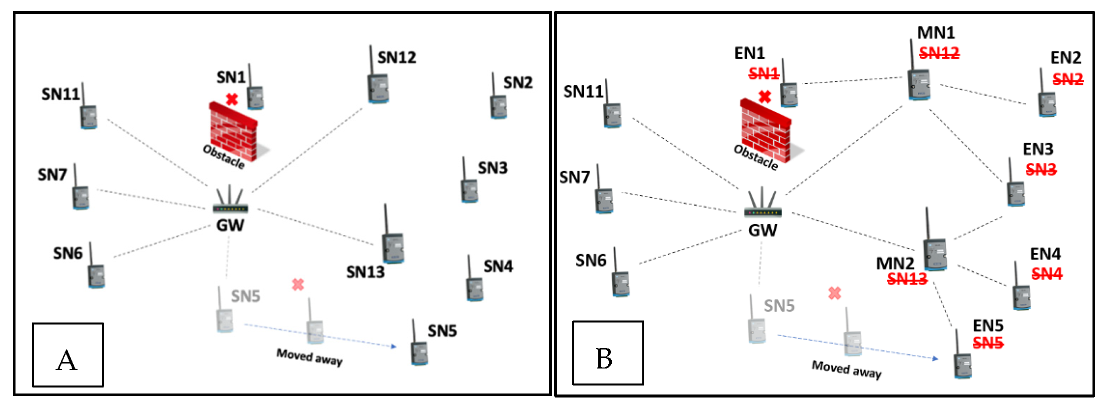
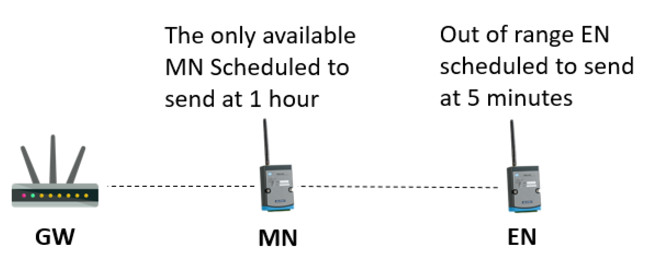
  • Every SN will wake up as intended/scheduled to try sending its message to the GW in normal Class A mode (maintaining normal Class A frequencies and duty cycle restrictions). If unsuccessful after three tries (no Acknowledgment message received), it will switch itself to a Class C mode (listening mode frequency). We label such blocked SN node as an EN.
  • If any SN is successful in reaching the GW, then (after transmitting its own message on Class A mode and receiving the corresponding successful Acknowledgement message from the GW) it will transmit a “rescue message” in the Class C frequency, in the hope that a nearby EN would receive it and reply within its normal Class C single receive window. We label such a node as an MN. This rescue message will include a chosen Class A frequency that an EN is expected to transmit its message on, and which this MN will be listening to during the “receive window”.
  • If steps 1 and then 2 are complete, and if an EN does receive a rescue message on the Class C frequency, it will transmit its message immediately within the normal “receive window” timing on the frequency stated in the rescue message. It will then stay in listening mode at this frequency until it receives an acknowledgement message via MN. Otherwise, if nothing is received within the user-defined timer (depending on the network transmission intervals), or if the MN is permanently removed from the network, the EN will start fresh again from step 1 (i.e., go back being SN, being in Class A, etc.) as this MN will be considered as an unreliable bridge.
  • If the MN does receive an EN message within the “receive window”, it will forward it to the GW as a normal Class A message and later it will also forward the Acknowledgment message back to the EN once received, using the pre-agreed frequency stated in the rescue message.
  • Both MN and EN nodes will go back to sleep and will wake up in Class A for the next scheduled time as in step 1.

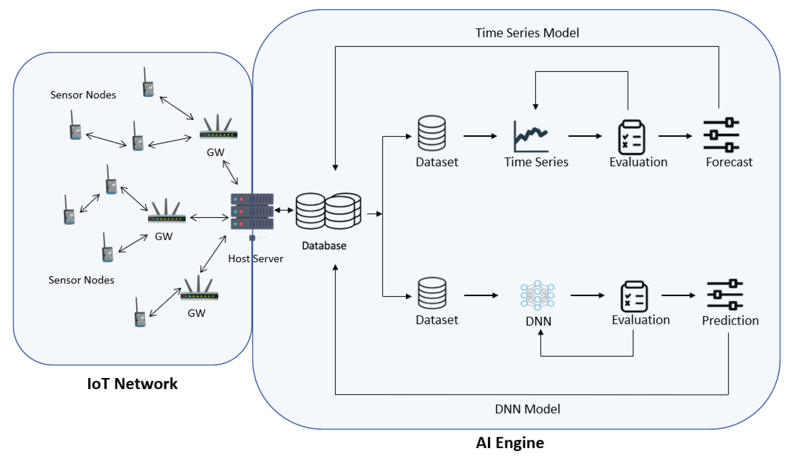
3.3. DXN Algorithms and Suitable AI Engine Implementation

We decided on implementing the following deployment scenario that reflects the issues mentioned in the problem statement in Section 3.2. As shown in Figure 2A, and as described in Section 3.2.2, this is a typical IoT network scenario that illustrates some SNs unable to reach the GW using LoRa. Specifically, SN2–SN4 are shown to be out of the GW range, therefore, they will switch to listening mode waiting for rescue messages. SN6–SN11 are directly communicating with the GW as they are within its range, and they are operating as regular LoRaWAN SNs. On the other hand, SN12 and SN13 are likely to become bridging SNs (MN1 and MN2) for SN2–SN4 as they are within their reach. Furthermore, SN1 was connected directly to the GW, but when an obstacle was introduced, it will become EN1 and will start communicating through its neighbour SN12 (MN1). As SN5 was moved away from the GW, it also becomes EN5 and started forwarding through SN13 (MN2). Figure 2B illustrates the deployment after the bridging algorithm took effect.
In consideration for the design of DXN, this scenario suffers from the following issues due to the geographical location and the transmission timing of the network nodes (see Section 3.2): (1) lack of MN selection mechanism, which cause an imbalance of the network load (power consumption eventually) due to the randomness of selecting the MN out of the available ones (if any); (2) lack of synchronisation mechanism (as it is costly to implement) and that will cause miscommunications; (3) high power consumption, due to the inconsistency in the transmission intervals which leads to long waiting time ENs spent in many cases waiting for a rescue message to be received. Therefore, we implemented our DXN engine to overcome these issues by using a Deep Neural Network (DNN) model [15] to predict the status/resources of each available MN. Then, based on that, it will assign a score for each MN; the better the resource, the higher the score will be for each MN. These scores will influence the MN selection in case more than one is available. DXN will keep monitoring the received messages and updating the scores as the MNs’ status changes so to choose the next MN for any new blocked SN (Figure 3).
The same DNN model is used to predict the time required for any chosen MN to forward a message for any specific EN and its corresponding reply/Ack message. This is to minimise the waiting (listening) time spent by the ENs (based on the connection status and the number of ENs available). The model will feedback the predicted timer for each bridged EN.
DXN also uses a Time Series model [16] in combination with its DNN to predict the SNs’ activity by forecasting the trend of their collected connectivity data to unify the transmission intervals for each chosen MN and its connected ENs (Figure 3).
For testing (see Section 3.4), DXN’s AI engine is trained using a dataset of the relevant data collected from all SNs messages in the IoT Network. This dataset contains around 6300 entries; each entry contains information about a packet received by the server from a specific SN (EN/MN). The dataset contains two types of information, first is the information provided by each node (such as node address, battery level, location, the role (EN, MN or just SN) and Tx interval), and the second is information calculated upon receiving the packet at the host server (receiving time, RSSI, SNR and time since the last packet). Each dataset was split into 80% for training and 20% for testing as it was the best effective use setup. Again, as illustrated in Figure 4, DXN is continuously making new decisions to improve the network performance. It follows a continuous cycle of analysing the collected data (the current network status), making new changes and then implementing them, and will start over by analysing the newly collected data (new network status) and so on.

3.4. DXN Tests Scenarios and Experiments

The following three test scenarios are designed to test the following three algorithms we implemented inside DXN: (a) Network Load-Based Optimisation Algorithm, (b) Network Activity-Based Optimisation Algorithm and (c) Nodes Transmission Scheduling Optimisation Algorithm. Furthermore, for our testing, we used the following hardware equipment: a single GW, MultiConnect Conduit gateway (MTCDT-LEU1), and SNs, MultiConnect mDots (MTDOT-868) (Figure 4). LoRaWAN 1.1 was the LoRa protocol version used in all of our tests. The maximum number of nodes used in our latest test was 13 SNs as they were enough to be deployed as regular LoRa SNs, ENs, and MNs. Each node was set to send a packet at 5 min interval, and the bridging algorithm will take effect when a node fails to reach the GW after three attempts. The time intervals are chosen to reduce the months run time of the actual scenario to obtain the results within a short time. For implementing the AI models, we used BigML, an online AI platform [17]. The DNN model was implemented with the following configurations: three hidden layers (64 neurons each), Adam algorithm, ReLU activation function and the weights were set automatically by BigML. Finally, for the Time Series model, a separated dataset was used that is arranged sequentially. BigML models time series data as a combination of components: level, trend, seasonality and error. For each component, it will be modelled additively, multiplicatively or not included at all. The training time was set to 6 h (eligible to end earlier if no further improvements can be achieved).

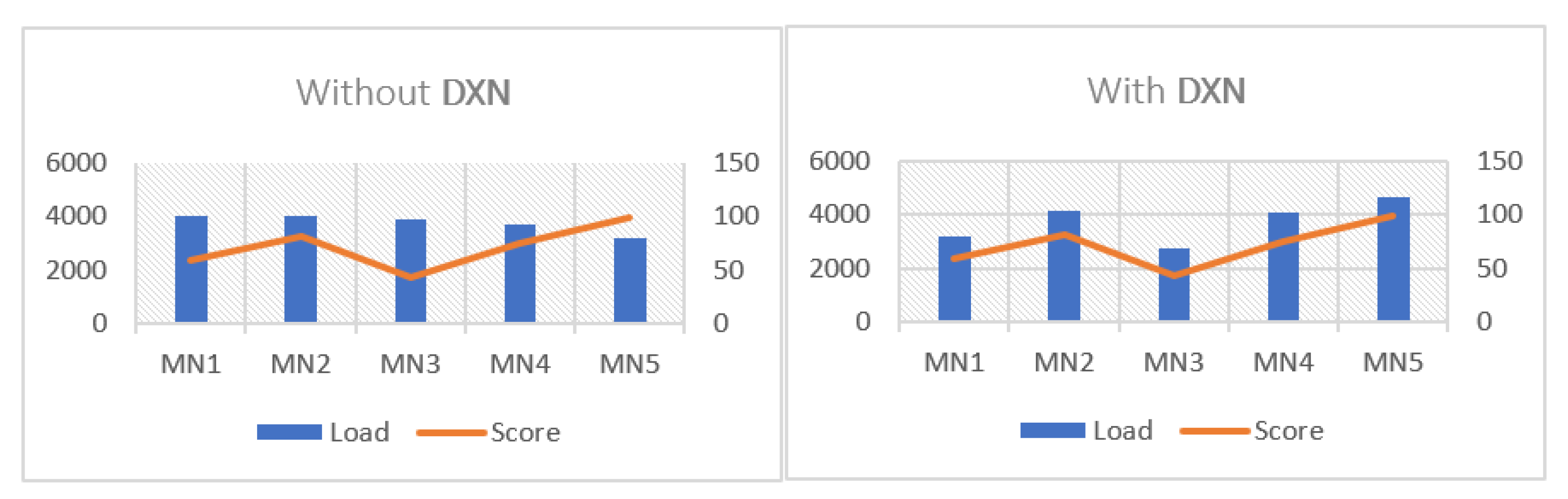
3.4.1. Network Load-Based Optimisation Algorithm

Using the DNN model, this algorithm is responsible for balancing the network load by selecting the best available MN at the time. This will take effect when an EN is within the range of more than one MN. In this case, DXN will select the MN with the higher score (better resources), and this helps balance the traffic in the network. In this case, all the heavy computations and analysis are performed at the host server leaving the node with minimum tasks. The selected MN’s address will be included in the downlink (Ack message from the GW to the EN); the EN will then only respond to that MN and will ignore any other MNs within its range.
To test this, we used a scenario that we have tested previously for better results comparison. The scenario, as shown in Figure 5, consists of two MNs (MN1 and MN2) and five ENs (EN1, EN2, …, N5). The nodes’ position is chosen so that MN1 is within EN1, EN2 and EN3′s range and MN2 is within EN3, EN4 and EN5′s range. This scenario was implemented to test the ability to create a bridge to link the GW to what was unreachable EN. However, this randomness will create an imbalance in the network, especially when MN1 and MN2 are transmitting at different intervals, leading to one of them having a higher chance of being selected by the EN. Since EN3 is within both MNs’ range, the selection is random based on which MN is discovered first (meaning, each time EN3 has something to send it will listen until the first rescue message from either MN1 or MN2 is received, and it will respond to that message).
In summary, with the use of DXN, each MN will now be given a score based on its current status, and EN3 will be instructed to respond to the one with the higher score (better resources) and will ignore messages received from others. Table 1 shows the difference in the EN3 behaviour between the two scenarios (with/without DXN).
From Table 1, it is clear that without DXN, EN3 is almost equally selecting between MN1 and MN2 (as both send at equal intervals) which, on paper, looks better balanced. However, by examining the MNs’ statistics, it shows otherwise (see Table 2). It shows that with the use of DXN, the forwarding capacity is spread between MN1 and MN2 unevenly, but according to the score, MN2 clearly has better resources and thus the added capacity.
To test the dynamic aspect of DXN, EN1 and EN2 (connecting through MN1) were removed during the test. This affected the MN1 score, since it had no ENs connecting through it, making its score higher than MN2′s score. EN3 then changed its behaviour and started to forward through MN1 since it had better recourses.
Another scenario was implemented to highlight the effect of the DXN engine on a larger network, where a total of five MNs and 11 ENs were deployed. The nodes were deployed in an arranged setup where almost every EN is within the range of more than one MN. The MNs’ scores were somewhat different. Figure 6 illustrates the difference between the scenario in Figure 5 with and without the DXN engine by showing the load (number of packets being forwarded) and the score for each MN. In addition, DXN creates a more balanced network when forcing MNs that have a higher score to forward more packets.

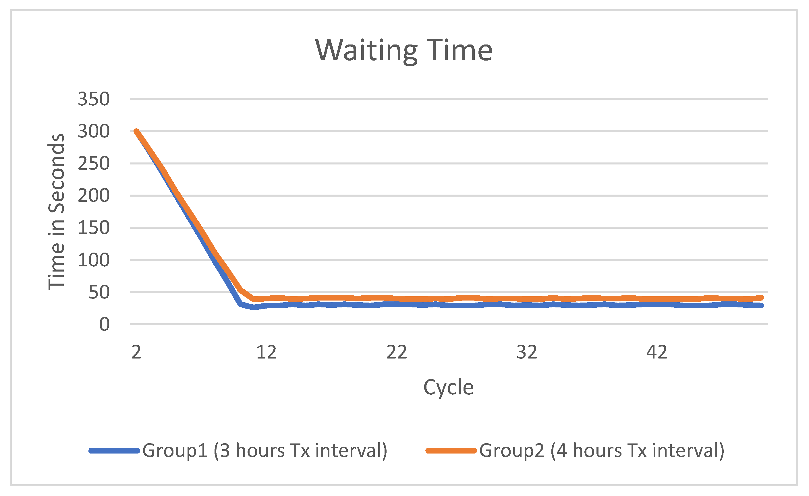
3.4.2. Network Activity-Based Optimisation Algorithm

As shown in Figure 7, EN was blocked but it is supposed to send a message every 5 min. The only available MN node is scheduled to send a message every 1 h. As it stands, EN will be waiting until MN wakes up every hour to forward its messages. DXN can see this situation from the host server data.
Therefore, the second part of DXN is performing two tasks. First, it will set a new Tx interval for both EN and MN in this scenario (using the DNN model). This Tx will force both to be active at similar times to reduce the listening time of EN and also the traffic generated from it. Second, it will study the collected data and continuously forecast new Tx intervals to both MN and EN based on the predicted trend of the received data (using the Time Series model). This is useful in seasonal applications where the collected data might matter more during specific periods of time. The new Tx interval of the MN will be reconsidered when load balancing, as well (change of the MN score). This might be applied to several groups of nodes based on their activity.
To test this part, the arrangement of Figure 5 is used. The transmitting intervals were set differently from SN to another and were set in specific different patterns. In addition, a delay was created manually to simulate the clock time drift at the SNs for rapid results obtaining and short experiment time. As shown in Figure 4, there are two MNs and five ENs with each nodes’ Tx intervals. The collected data at the host server that DXN saw for each group and the new adjustments are as shown in Table 3.
As shown in Table 3, the new Tx interval for group 1 is set to 8 h, meaning each node will transmit its message every 8 h including MN1, and for group 2, the new Tx interval is now 6 h. It is also noticeable that MN1′s score was 59, and now that it is sending more often (every 8 h instead of previously every 12 h), that will affect its power consumption and thus its score, which dropped to 55. Meanwhile, the score of MN2 remained the same because the new Tx interval of its group (group 2) was set to 6 h (meaning, nothing is going to change in the MN2 status). Figure 8 shows the results of this normalisation process by DXN.

3.4.3. Nodes Transmission Scheduling Optimisation Algorithm

To enhance the communication of any IoT network further is to make all its SNs work in a synchronised schedule. DXN is designed to achieve this by including synchronisation data in the downlink messages from the host server to all the SNs. Effectively, DXN is overriding the duty cycle restriction in LoRaWAN networks (implemented on the 868 MHz band). This way, no “intelligent SNs” are needed.
DXN set up “continuously updated timers” that will be included at each rescue message to be used by the SNs to schedule their waking up and sleeping behaviour as follows. DXN will decide on the rescue message intervals in an optimum way by balancing between increasing the interval for as long as possible and ensure the minimum wake-up time by the ENs. MNs will repeat sending the rescue message to all blocked nodes it is serving (meaning, when an EN replies to a rescue message and failed to receive an Ack, it will try again after this timer is finished. DXN predicts this timer based on analysing the communication information). This is to overcome the duty cycle limitations (predicting when the channel will be available again).
The scenario in Figure 5 is also used to test this scheduling mechanism. To ensure successful communication between the SNs in each group, MNs were set to a five-minute rescue message interval. The GW Ack message will include this timer which will keep being updated by DXN and the new rescue message repeat timer. ENs, on the other hand, at the first cycle, was set to the maximum timer (5 min) to ensure the reception of the rescue message. Once they receive a rescue message and their packet is acknowledged by the GW, the Ack will include the new rescue message interval as per the previous step. Further, on the following cycles, each EN will report its waiting time, and DXN will ensure the minimum waiting time while maintaining a successful connection. The goal is to reduce the waiting time of EN to the minimum, and so for this test, we chose the waiting time for each EN to be 30 s (the time from waking up until receiving the rescue message is 30 s). To ensure a successful packet delivery, the change is set to be gradual rather than immediate. Figure 9 details the waiting time at each of the two groups in Figure 5. Note that group1 and group2 were set to 3 h and 4 h uplink intervals, respectively. In this case, DXN changes group2 timers more gradually than group1 since each node in group2 has more sleeping time, leading to a higher chance of miscommunicating.
As shown in the figure above, after around 10 cycles of scheduling by DXN, the ENs in each group were settled on the waiting time goal of around 30–40 s based on the groups’ Tx interval, with a staggering reduction of around 86% in group2 and 90% in group1, compared to the first cycle with the initial rescue message interval of 5 min.

3.4.4. Overall Evaluation of DXN

DXN has shown that it is possible to enhance the network performance by implementing a dynamic AI-based engine that is constantly analysing the collected data from the actual deployed SNs and giving live feedback to adjust the SNs’ behaviour. This was achieved by using the DNN model with 98% accuracy in predicting. As for the Time Series model, it achieved a Mean Squared Error (MSE) of 0.11.
By using the network server resources located in the cloud (assumed to be unlimited in terms of power source, computational capabilities, storage, etc.), DXN was able to perform all the heavy calculations, leaving the SNs with minimum tasks and eliminating any additional overhead when compared to solutions such as [14] and [18] that are proposing the implementation of AI algorithms onboard the deployed SNs. Furthermore, no additional hardware equipment/capabilities were required other than the typical LoRaWAN compatible network. Therefore, we envisage that more enhancement is achievable by including extra (simple) information within the SNs’ data messages.

4. Conclusions

DXN has shown better performance in terms of (1) node availability due to load balancing, and (2) better node longevity (reduced battery consumption by sending nodes to sleep) by reducing the waiting time for each node and by grouping the nodes based on their activity. These aspects are often difficult to maintain even in well-designed and planned IoT networks due to unexpected challenges that might take place after the network deployment. DXN is achieved by using an AI-based engine that is based on simple Time Series and DNN models capable of analysing the collected data from the nodes and predicts changes to the behaviour of the nodes, something that can be added to enhance all IoT networks.
By reviewing the AI literature in LPWAN IoT networks, we noticed that AI is mostly implemented in a fixed way, yet, as DXN demonstrated, it has the potential to be utilised dynamically for powerful prediction capabilities. We believe that the future of IoT lies with utilising the LPWAN networking capabilities combined with AI self-learning benefiting from the cloud resources.

Author Contributions

Data curation, A.A.; Investigation, A.A.; Methodology, A.A.; Supervision, I.L.; Validation, A.A.; Writing—original draft, A.A.; Writing—review & editing, I.L. All authors have read and agreed to the published version of the manuscript.

Funding

This research received no external funding.

Institutional Review Board Statement

Not applicable.

Informed Consent Statement

Not applicable.

Data Availability Statement

The datasets generated during the current study are available from the corresponding author upon reasonable request.

Acknowledgments

Special thanks to the University of Basra, the Iraqi Ministry of Higher Education and Scientific Research (MO-HESR) for sponsoring this Ph.D. study and to Russell IPM Ltd. for their cooperation, providing data and testing equipment.

Conflicts of Interest

The authors declare no conflict of interest.

References

  1. Atlam, F.H.; Walters, R.J.; Wills, G.B. Intelligence of things: Opportunities challenges. In Proceedings of the 2018 3rd Cloudification of the Internet of Things (CIoT), Paris, France, 2–4 July 2018. [Google Scholar] [CrossRef] [Green Version]
  2. Mikhaylov, K.; Petäjäjärvi, J.; Haenninen, T. Analysis of the Capacity and Scalability of the LoRa Wide Area Network Technology. In Proceedings of the European Wireless 2016, 22th European Wireless Conference, Oulu, Finland, 18–20 May 2016. [Google Scholar]
  3. Petajajarvi, J.; Mikhaylov, K.; Hamalainen, M.; Iinatti, J. Evaluation of LoRa LPWAN technology for remote health and wellbeing monitoring. In Proceedings of the International Symposium on Medical Information and Communication Technology, ISMICT, Worcester, MA, USA, 20–23 March 2016. [Google Scholar] [CrossRef]
  4. Petäjäjärvi, J.; Mikhaylov, K.; Roivainen, A.; Hänninen, T.; Pettissalo, M. On the coverage of LPWANs: Range evaluation and channel attenuation model for LoRa technology. In Proceedings of the 2015 14th International Conference on ITS Telecommunications, ITST 2015, Copenhagen, Denmark, 2–4 December 2015; pp. 55–59. [Google Scholar] [CrossRef]
  5. Tsiropoulou, E.E.; Paruchuri, S.T.; Baras, J.S. Interest, energy and physical-aware coalition formation and resource allocation in smart IoT applications. In Proceedings of the 2017 51st Annual Conference on Information Sciences and Systems, CISS 2017, Baltimore, MD, USA, 22–24 March 2017. [Google Scholar] [CrossRef]
  6. Zhou, W.; Tong, Z.; Dong, Z.Y.; Wang, Y. Lora-hybrid: A LoRaWAN based multihop solution for regional microgrid. In Proceedings of the 2019 IEEE 4th International Conference on Computer and Communication Systems, ICCCS 2019, Singapore, 23–25 February 2019; pp. 650–654. [Google Scholar] [CrossRef]
  7. Holin, N.; Sornin, F. LoRaWAN Relay Workshop. In Proceedings of the Thing Network Conference, Amsterdam, The Netherlands, 31 January–1 February 2019. [Google Scholar]
  8. Jeon, J.; Park, J.H.; Jeong, Y.S. Dynamic Analysis for IoT Malware Detection with Convolution Neural Network Model. IEEE Access 2020, 8, 96899–96911. [Google Scholar] [CrossRef]
  9. Zeiler, M.D.; Fergus, R. Visualizing and understanding convolutional networks. In Lecture Notes in Computer Science (including subseries Lecture Notes in Artificial Intelligence and Lecture Notes in Bioinformatics); Springer: Cham, Switzerland, 2014; Volume 8689, pp. 818–833. [Google Scholar] [CrossRef] [Green Version]
  10. Rahimi, P.; Chrysostomou, C. Improving the Network Lifetime and Performance of Wireless Sensor Networks for IoT Applications Based on Fuzzy Logic. In Proceedings of the 15th Annual International Conference on Distributed Computing in Sensor Systems, DCOSS 2019, Santorini, Greece, 29–31 May 2019; pp. 667–674. [Google Scholar] [CrossRef]
  11. Heinzelman, W.R.; Chandrakasan, A.; Balakrishnan, H. Energy-efficient communication protocol for wireless microsensor networks. In Proceedings of the 33rd Annual Hawaii International Conference on System Sciences, Maui, HI, USA, 7 January 2000; p. 223. [Google Scholar] [CrossRef]
  12. Puschmann, D.; Barnaghi, P.; Tafazolli, R. Adaptive Clustering for Dynamic IoT Data Streams. IEEE Internet of Things J. 2017, 4, 64–74. [Google Scholar] [CrossRef] [Green Version]
  13. Zhang, C.; Dong, M.; Ota, K. Enabling Computational Intelligence for Green Internet of Things: Data-Driven Adaptation in LPWA Networking. IEEE Comput. Intell. Mag. 2020, 15, 32–43. [Google Scholar] [CrossRef]
  14. Kumari, P.; Gupta, H.P.; Dutta, T. A Bayesian Game Based Approach for Associating the Nodes to the Gateway in LoRa Network. IEEE Trans. Intell. Transp. Syst. 2021. [Google Scholar] [CrossRef]
  15. Deep Neural Network—An Overview|ScienceDirect Topics. Available online: https://www.sciencedirect.com/topics/computer-science/deep-neural-network (accessed on 9 April 2021).
  16. Time Series Models—An Overview|ScienceDirect Topics. Available online: https://www.sciencedirect.com/topics/neuroscience/time-series-models (accessed on 9 April 2021).
  17. BigML. Available online: https://bigml.com/ (accessed on 6 May 2021).
  18. Kwon, M.; Lee, J.; Park, H. Intelligent IoT Connectivity: Deep Reinforcement Learning Approach. IEEE Sens. J. 2020, 20, 2782–2791. [Google Scholar] [CrossRef]
Figure 1. Screenshot of the database used by DXN at the host server.
Signals 02 00035 g001
Figure 2. (A) The implemented IoT network deployment, (B) The same deployment with the bridging algorithm.
Signals 02 00035 g002
Figure 3. Overall DXN showing the “AI Engine” and the “IoT Network” blocks.
Signals 02 00035 g003
Figure 4. Network hardware.
Signals 02 00035 g004
Figure 5. Load balance scenario.
Signals 02 00035 g005
Figure 6. DXN load balance with 5 MNs scenario.
Signals 02 00035 g006
Figure 7. Different Tx intervals scenario.
Signals 02 00035 g007
Figure 8. Tx interval adjustment for messages by DXN.
Signals 02 00035 g008
Figure 9. Waiting time reduction using DXN.
Signals 02 00035 g009
Table 1. The effect of DXN on EN3 behaviour.
EN#Total Tx PacketsWithout DXNWith DXN
Packets through MN1Packets through MN2Successful Delivered PacketsPDRAvg. Overall Tx Time (sec)Packets through MN1Packets through MN2Successful Delivered PacketsPDRAvg. Overall Tx Time (s)
EN311525695831152100%4.1-1152115199.9%4.8
Table 2. DXN load balance based on the score.
MN#Without DXNWith DXNScore
Packets Sent to GWPackets Forwarded to GWTotal Packets SentCapacity PercentagePackets Sent to GWPackets Forwarded to GWTotal Packets SentCapacity Percentage
MN1115228734025349%115223043456300%59
MN2115228874039350%115234564608400%82
Table 3. Tx interval adjustment by DXN.
Group#NodesTx Interval (Hours)MN ScoreNew Tx Interval (Hours)New MN Score
Group1MN11259855
EN13
EN210
Group2MN2682682
EN311
EN45
EN54
Publisher’s Note: MDPI stays neutral with regard to jurisdictional claims in published maps and institutional affiliations.

