1. Introduction
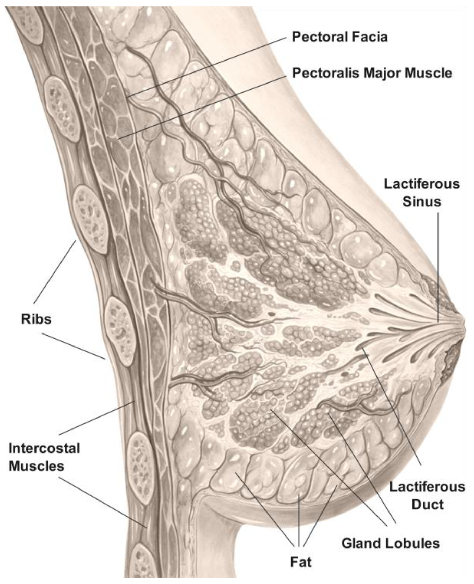
Breast density is considered to be a measure of fibrous and glandular tissue existence (also known as fibroglandular tissue) in the whole breast when compared to the fat tissue. It has no direct relation to the breast size or its firmness. There are three basic components of a breast: connective tissue, ducts, and lobules. The connective tissue, which is formed of fatty and fibrous tissue, envelops and holds everything in place. Lobules are the small glands that produce milk, while ducts are the tiny transport tubes that carry milk from the lobules to the nipple. Together, lobules and ducts are known as glandular tissue (
Figure 1). Fibrous tissue and fat give breasts their size and shape while they also hold the rest of the breast components in place. Most breast cancers begin in the ducts or lobules. Breast density as a measurement is important mainly for two reasons: Women who have dense breast tissue, present a higher risk of developing breast cancer compared to women with less dense tissue. It is unclear until now why high density is associated with higher breast cancer risk. This may be attributed to the fact that dense breast tissue is formed by a bigger proportion of cells that could be evolved into abnormal under some conditions. The absolute relationship between the risk factor of breast cancer development in women with increasing breast mammographic density has already been reported in many relevant studies [
1].
The second reason is that dense breast tissue (fibrous and glandular) makes it harder for radiologists to detect cancerous regions in mammograms because it looks white or opaque on an MRI. Breast masses and cancerous regions also share the same dominant white characteristics as the rest of the healthy tissue, so density makes it harder for the abnormalities to be traced by radiologists or computer assisted diagnosis (CAD) systems. In contrast, a fatty tissue looks almost black, so it is easier to see abnormalities that have large intensity values in a low intensity background. In screening mammography, according to the American College of Radiology Breast Imaging Reporting and Data System (ACR BI-RADS), there exist four different levels of density [
2]. Almost entirely fatty indicates that breasts are almost entirely composed of fat (ACR-A). Scattered areas of fibroglandular density indicate there are some scattered areas of density, but most of the breast tissue is non-dense (ACR-B). Heterogeneously dense indicates that there are some areas of non-dense tissue, but most of the tissue is dense (ACR-C). Finally, extremely dense indicates that nearly all breast tissue is dense (ACR-D).
Breast density cannot be detected through physical examination but only through mammography, and it is an important variable that affects the sensitivity of mammography [
3,
4,
5,
6]. Over 40% of women with dense breast tissue are characterized as heterogeneously dense (ACR-C) or extremely dense (ACR-D). Dense breast tissue is an independent risk factor for the development of abnormalities and decreases the likelihood of breast cancer being detected successfully on screening mammography, leading potentially to delayed diagnosis, which can have detrimental results.
In order to automatically identify and categorize breast lesions in mammograms using traditional machine learning models and to bring these results to doctors’ attention, computer-aided detection systems (CAD) were developed in the 1990s [
7,
8,
9]. Yet, due to their low specificity, current conventional CAD systems are unable to considerably increase screening performance. The success of these algorithms to identify and categorize abnormalities in mammograms is related to specificity. This differs from diagnosis, which draws conclusions about the cause of an aberration. It is crucial to find irregularities in mammograms, which could be caused by mistakes or tired observers. Convolutional neural networks (CNNs) have gained popularity in recent years for a variety of image processing classification tasks. CNN-based CAD systems have proven to be quite effective, with high rates of breast cancer diagnosis. However, there are still some open issues in the automatic breast cancer detection problem, one of the most important being the breast density as already described earlier.
In the literature, the use of generative adversarial networks (GANs) for numerous medical challenges, including data synthesis and augmentation, is constantly growing. However, these models may experience numerous artifacts (i.e., checkerboard artifacts), which may affect the quality of the final synthesized images, especially when working with full-size mammograms. GANs can help in the synthesis of a variety of plausible-looking mammography images either in full size [
10,
11,
12,
13] or in ROI-based approaches [
14,
15].
Due to its impact on the accurate detection of cancer in mammograms, the problem of automatic breast tissue recognition has been extensively studied over the last decade, with a large number of papers published in this area proposing systems that use either traditional machine learning techniques or, more recently, deep learning networks and architectures [
4,
5,
6,
7,
13,
15,
16]. However, to our knowledge, none of them proposes a method to “transform” breast density to lower density levels and thus enhance the diagnostic accuracy of CAD systems.
Motivated by the crucial role that breast tissue density plays in the detection of breast cancer, as it makes it more challenging for radiologists to accurately detect cancerous regions in mammograms, we sought to investigate to what extent computer-assisted diagnosis systems are affected by this challenge, using different types of mammograms ranging from scanned film to fully digital images in our experiments. To address this, we propose a novel breast tissue transformation using CycleGAN network topology that can be applied to any region of interest (ROI) to adjust its density to match the characteristics of an ACR-A class tissue, which is easier to diagnose successfully. CycleGAN was chosen due to its widespread applications and accomplishments in the field of cancer imaging [
16]. A crucial methodological characteristic of CycleGAN is that it can train on unpaired data without the need for matching image pairings in the source and target domains. As our datasets lack image pairings and the same patient’s breast cannot belong to both the high and low breast density domains, using unpaired training data confirmed that CycleGAN would work with our datasets. The main contribution of our system is taking breast density into account, and by using a CycleGAN model, transforming the density of the ROI’s tissue to match the characteristics of an ACR-A class tissue. This process significantly improves recognition accuracy while reducing the number of undetected ROIs due to their dense breast tissue.
The structure of the paper is as follows: In
Section 2, we give a detailed description of the proposed CAD system. We present the different modules that it consists of and the different datasets that were used to test the efficacy of the system. In
Section 3, we present the experimental setup and results, which are further discussed and commented in
Section 4. Finally, in
Section 5, some conclusions and remarks are given concerning the limitations and further research.
2. The Proposed System Overview
The main objectives of this work are summarized as follows:
Development of a novel approach/method to detect hidden suspicious abnormalities in ROIs that are partially or completely masked by surrounding tissue by taking into account the local breast density as recognized by a CNN classifier that marks the tissue ACR into four levels (A, B, C, D).
Elimination of the masking effect due to the surrounding tissue on the examined ROI by transforming the ROI’s ACR level into the A category. This procedure is achieved using a GAN/CycleGAN topology that cycles through the ACR levels.
Improvement of the overall abnormal region detection performance using a CNN network architecture based on a fine-tuned VGG16 network and extended tests on five of the most well-known datasets in the field.
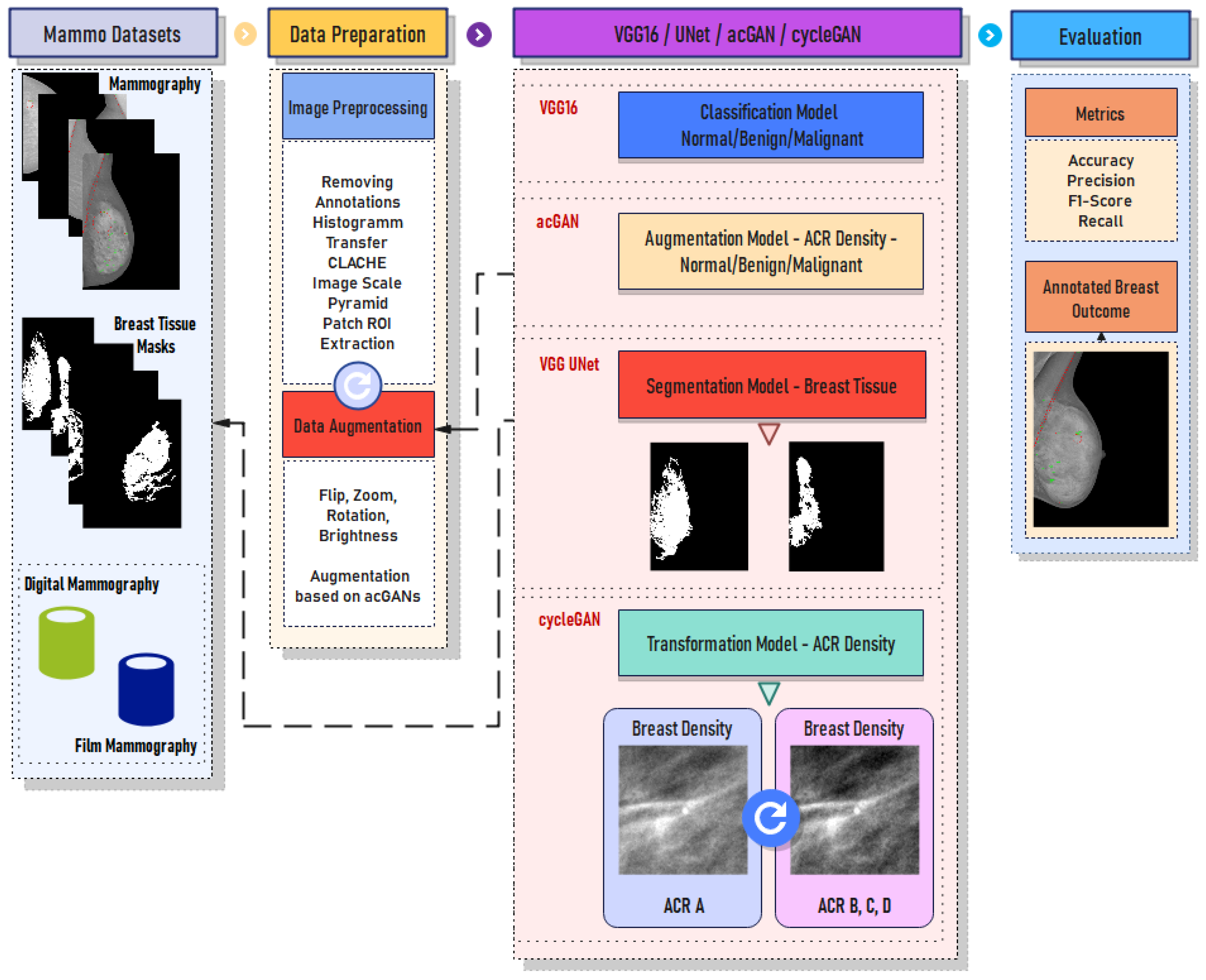
The proposed CAD system used in this work is illustrated in
Figure 2. It consists of three main modules: (a) the data preparation module where image preprocessing and data augmentation take place, (b) the deep learning module where breast tissue segmentation, breast density transformation, and suspicious region detection are performed, and finally, (c) the evaluation module where annotation of abnormal regions on the given mammogram under examination is performed. To make our system more robust and to consider the different types of mammograms acquired during examination (fully digital, as well as scanned X-ray film), we thoroughly tested our system using five different datasets containing digital and film-scanned mammograms.
- A.
The VinDR-Mammo dataset (digital)
The VinDr-Mammo [
17] dataset is a large-scale dataset of full-field digital mammograms consisting of 5000 four-view examinations accompanied by breast-level assessments and findings annotations. To the best of our knowledge, VinDr-Mammo is currently the largest public dataset (containing approximately 20,000 scans) of full-field digital mammograms that also provides breast-level BI-RADS assessment categorization together with suspicious or possible benign findings that require follow-up examination as well as ACR breast tissue/finding level annotations.
- B.
The SuReMaPP dataset (digital)
The SuReMaPP [
18], published recently, consists of 343 mammograms that have been hand-labeled by expert radiologists to identify suspicious regions, such as abnormalities (benign and malignant) and calcifications. SuReMaPP contains mammograms with ACR keyword descriptions that are corresponding to the ACR BI-RADS specification.
- C.
The MIAS dataset (film)
The Mammographic Image Analysis Society (MIAS) [
19] dataset consists of 322 film mammograms (106 fatty and 216 dense images). Annotations are given in a separate file containing the background tissue type, the class and the severity of the abnormality, x and y coordinates of the center of the irregularities, and the approximate radius of a circle enclosing the abnormal region in pixels. For this dataset, there is no annotation for ACR breast tissue level.
- D.
The DDSM dataset (film)
The digital database for screening mammography (DDSM) [
20,
21,
22] is provided by the University of South Florida. It contains film mammograms, which are digitized using four different types of digitizers. The database contains approximately 2500 studies. Each study includes two images (views) of each breast, as well as some associated patient information (age at time of study, ACR breast density rating, subtlety rating for abnormalities, and ACR keyword description of abnormalities) and image information (scanner used for the digitization, scanner spatial resolution, etc.). The ACR keyword description of the database was matched to the ACR BI-RADS categorization.
- E.
The INbreast dataset (digital)
The INbreast dataset [
23] was used in the training phase of our CNN-based CAD system (patch extraction-based approach) and as a golden standard in all our experiments. The other datasets were used to evaluate the performance of the proposed system under different types of acquired mammograms.
2.1. Data Preparation
2.1.1. Input Image Normalization
To eliminate the differences in the intensity levels of the mammograms used in the databases, the histogram transfer method was applied from the INbreast dataset to all other images. This normalization preprocessing step in CAD systems is crucial as it can account for large intensity variations that are typically attributed to the use of different scanners with varying parameters in the image-capturing process. These intensity variations can also severely affect the performance of processing and analysis steps, such as image registration, segmentation, and tissue volume estimation. To ensure objective image comparison between different mammograms, a normalization algorithm is performed in advance to modify the distribution of intensity values of each scan and match the selected baseline image. This preprocessing step was adopted from [
24].
In order to help radiologists detect abnormalities, the adaptive histogram enhancement (AHE) [
25,
26] method is typically applied as a preprocessing step in CAD systems. The AHE method is a contrast-boosting technique that enhances local contrast and image details. Medical images can benefit greatly from this preprocessing step, but it can also generate a lot of noise as a side effect. To increase the image contrast and eliminate the noise enhancement, a variation known as the contrast-limited adaptive histogram equalization (CLAHE) technique [
27,
28,
29] is used, as proposed in the literature.
2.1.2. Image/Breast Tissue Segmentation
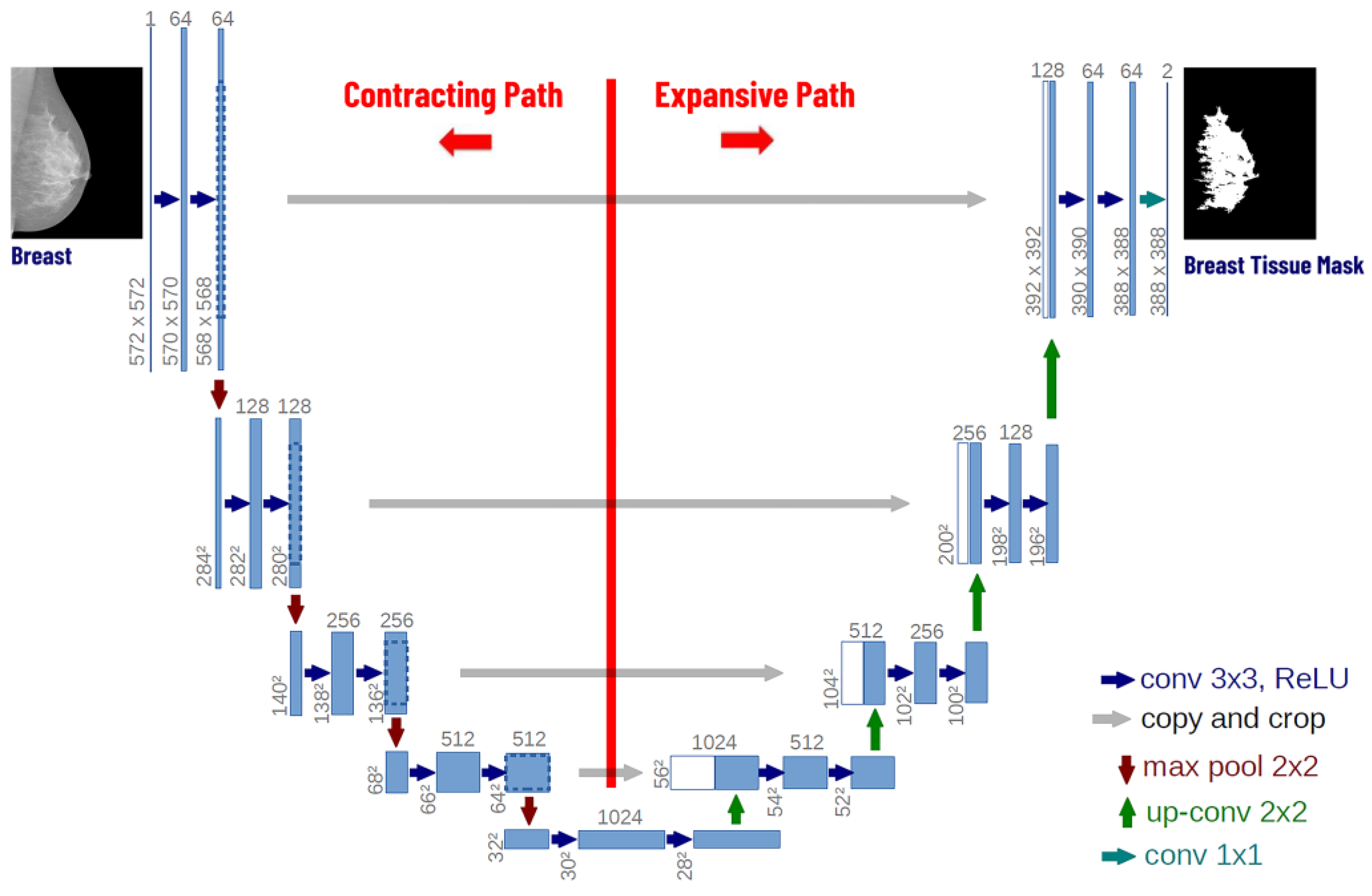
To perform breast tissue segmentation, we estimate the tissue masks using a VGG-UNET network. The UNET architecture was initially proposed by Ronneberger et al. [
30] for biomedical image data segmentation. We trained the VGG-UNET network using the images from the INbreast dataset and then applied the learned model to images from other datasets. For the segmentation step, we replaced the UNET encoder with a pre-trained VGG16 encoder, as depicted in
Figure 3. The reason for this is that the VGG16 is already pretrained on the ImageNet dataset, whereas the UNET encoder would have to be trained from scratch to learn the features and the breast tissue area characteristics with significantly lower performance. Finally, the VGG16 encoder is converted into a symmetrical UNET architecture. We applied the constructed model to all datasets (except INbreast), to extract the tissue regions that will be used in the following analysis steps (
Figure 3).
2.2. The Deep Learning Module
2.2.1. Feature Extraction/Classification
In the literature, many techniques for feature extraction have been proposed. In recent years, deep convolutional neural networks (DCNNs) have attracted great attention due to their outstanding performance. In image classification issues, including image analysis as in [
31,
32], CNNs have been proven to be successful. A convolutional neural network (CNN) is made up of a series of trainable stages stacked on top of one another, a supervised classifier, and feature maps [
33].
Transfer learning is used on our first model, which is based on the VGG16 architecture. The model was pre-trained on ImageNet, and the first four blocks of residual layers were kept frozen, except for the batch normalization (BN) layers, which required retraining to achieve better convergence. By applying transfer learning, a model can be trained using smaller sets of training data while still being capable of accurate predictions, mostly due to the learned parameters from the source model (in our case the pretrained ImageNet). An additional fully connected (FC) layer with a size of 1024 is added to the overall architecture, followed by a dropout regularization layer to ensure generalization performance. For the output layer, a final FC layer is added. Our model has three output classes: normal, benign, and malignant. This model, which we will refer to as VGG16-NBM, is used to categorize each image patch from the entire breast MRI as either normal, benign, or malignant.
A similar VGG16 model was also constructed with four outputs corresponding to the four different categories of breast density: ACR-A, ACR-B, ACR-C, and ACR-D. Similar approaches have also been reported in the literature that perform very well [
34]. We will refer to this model as VGG16-ACR, and its task is to recognize the density class for each image patch.
For the training of the two VGG16-based models (VGG16-NBM and VGG16-ACR), the INbreast database was used. The input to the VGG16 models is patches the size of 256 × 256 pixels. To augment our training set, we exploited the capability of GAN topologies to produce artificial samples of a specific domain as presented in the following section.
2.2.2. Generative Adversarial Networks (GANs)
Recently, the idea of adversarial training has gained popularity, and deep learning research has advanced significantly. Since their initial presentation, generative adversarial networks (GANs) have attracted attention worldwide, and every year, even more studies are published and presented in different research areas, especially in medical image analysis. GANs have been used for data augmentation in several recent works [
35,
36,
37,
38,
39], including medical image analysis.
Generally, training on a set with a large number of samples, performs well and gives high accuracy rates. However, biomedical datasets usually contain only a relatively small number of samples due to the limited number of patients that can be involved in different studies. To solve this problem, data augmentation can be used to increase the size of the input data by generating new data from the original input data. Given the rapid progress of generative models in synthesizing realistic images and the known effectiveness of simple data augmentation techniques (e.g., horizontal flipping, rotation, shifting, brightness adjustments), we have integrated two GAN models in our CAD system to synthetically augment the extracted patches from the training database. In this way, we can balance the class ratio of normal, benign, and malignant samples in the training set.
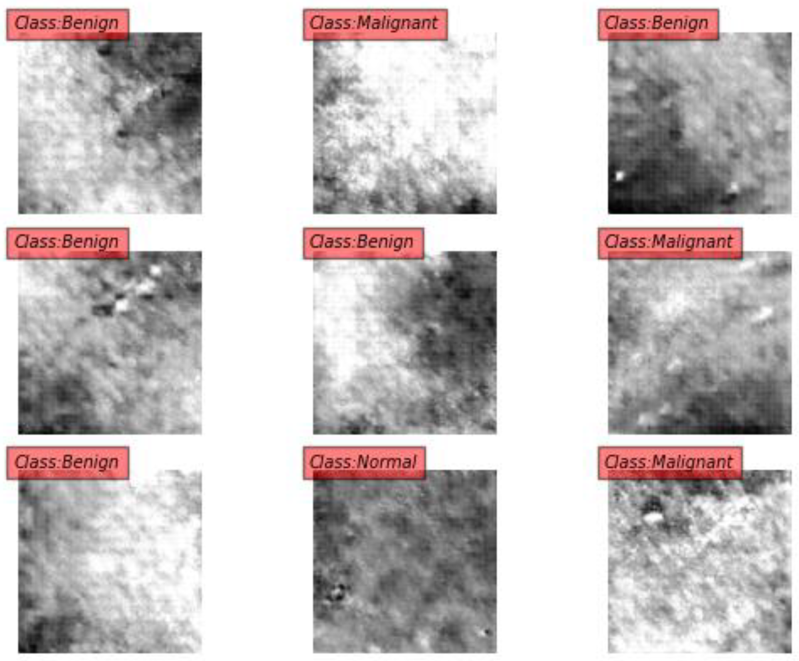
The first GAN (GAN-NBM) was used to produce synthetic patches from normal/benign/malignant classes to ensure the robustness of the CNN-based classifier and variability of the samples. The second one (GAN-ACR) was implemented to produce synthetically augmented patches belonging to the four different tissue ACR categories.
Figure 4 and
Figure 5 depict patches generated by the GAN model that belong to the specified classes. In
Figure 4, the GAN-NBM produces ROI patches from the normal, benign, and malignant classes. In
Figure 5, ROI patches representing the ACR breast density class are generated. The role of both GANs is to augment the training dataset in an unsupervised manner. For both cases, the INbreast annotation, which refers to the annotation of masses and microcalcifications in mammograms, was used, imposing at least an 85% ratio of overlap with the breast tissue mask that was estimated from the previous image segmentation step, especially for the patches of classes ACR-A, -B, -C, and -D.
2.2.3. CycleGANs
CycleGANs are used to train an image-to-image translation model, which does not depend on paired datasets to learn the mapping between the input and the output images [
40]. The key to CycleGAN’s success is the idea of an adversarial loss that forces the generated images to be, in principle, indistinguishable from real images. In our work, we adopt the architecture of CycleGAN as proposed by Johnson et al. [
41], which has shown impressive results for neural-style transfer and super-resolution. Formally, given a source domain X and a target domain Y, CycleGAN aims to learn the mapping of G: X → Y between input and output images such that the G(X) is the translation of the image from domain X to domain Y. Additionally, it also aims to learn a reverse mapping of F: Y → X such that F(Y) is the translation of the image from domain Y to domain X.
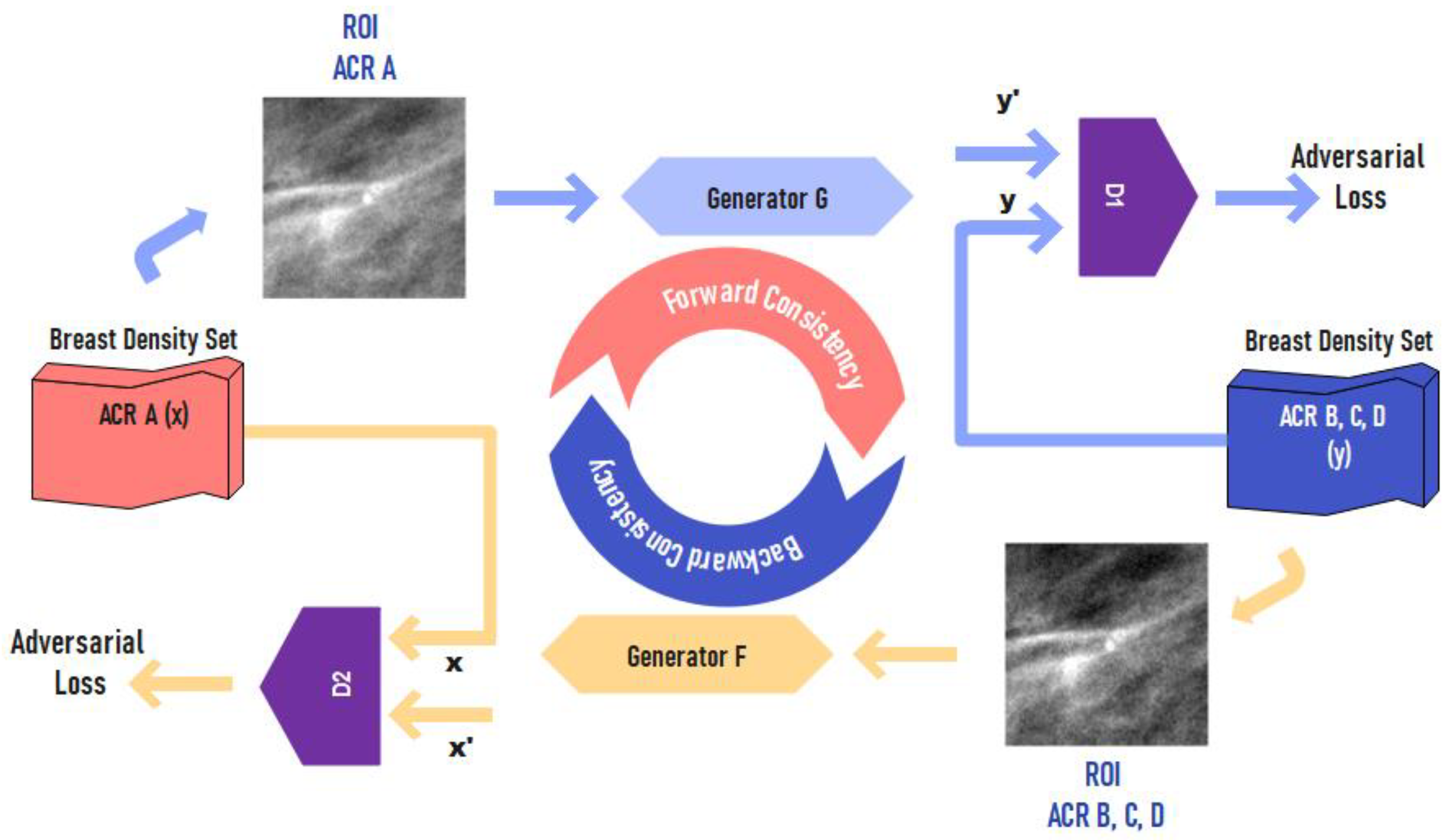
In our work, the CycleGAN model is used to transform patches from classes (domain) ACR-B, -C, and -D to class ACR-A. The main purpose of this model is to subtract the effect of tissue masking from the breast patches and transform their tissue into class ACR-A. The training of the CycleGAN was performed after creating data belonging to two categories: one containing image patches from class ACR-A and the other constructed by considering all the remaining patches from classes ACR-B, ACR-C, and ACR-D (
Figure 6).
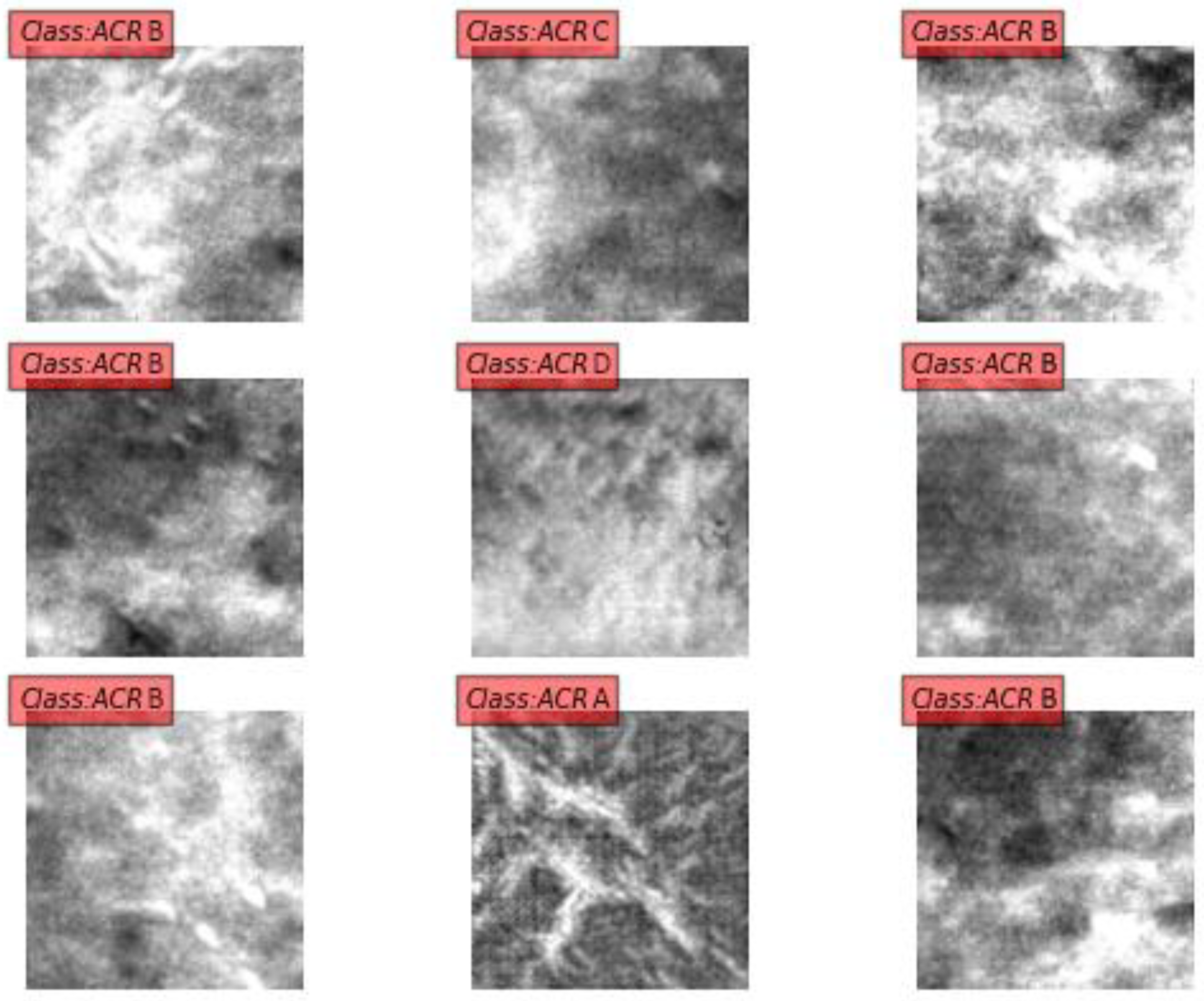
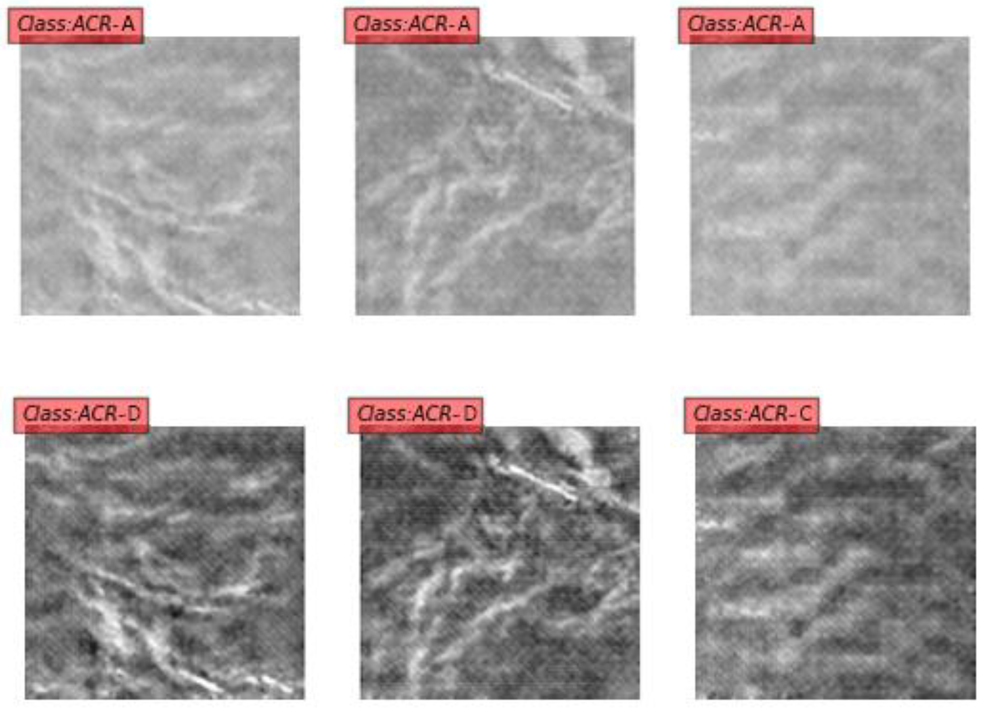
In
Figure 7 and
Figure 8, patches from the unpaired categories ACR-A, ACR-B, -C, and -D are shown. The ROI patches in the first row of
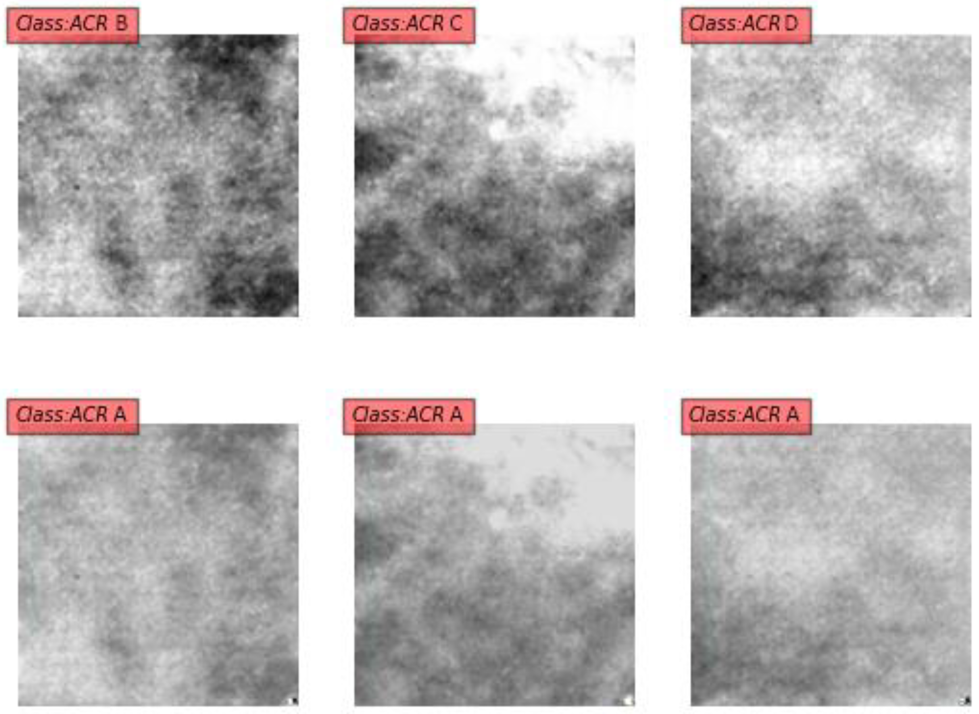
Figure 7 (belonging to classes ACR-B, ACR-C, and ACR-D) are transformed to the corresponding class ACR-A patches in the second row using the CycleGAN model. In
Figure 8, the opposite transformation is depicted. Due to the cycle consistency characteristic of CycleGAN, we can also transform ACR-A patches back to the ACR-A class, thereby examining the convergence of the model (
Figure 9).
Since data from this categorization are highly unbalanced, the GAN-ACR model described in the previous section was used to produce synthetic data up to a total of 10 million patch images. The CycleGAN was left for several epochs to run (in each epoch the network uses a pair of 10 million image patches, which are randomly shuffled at the end of each epoch).
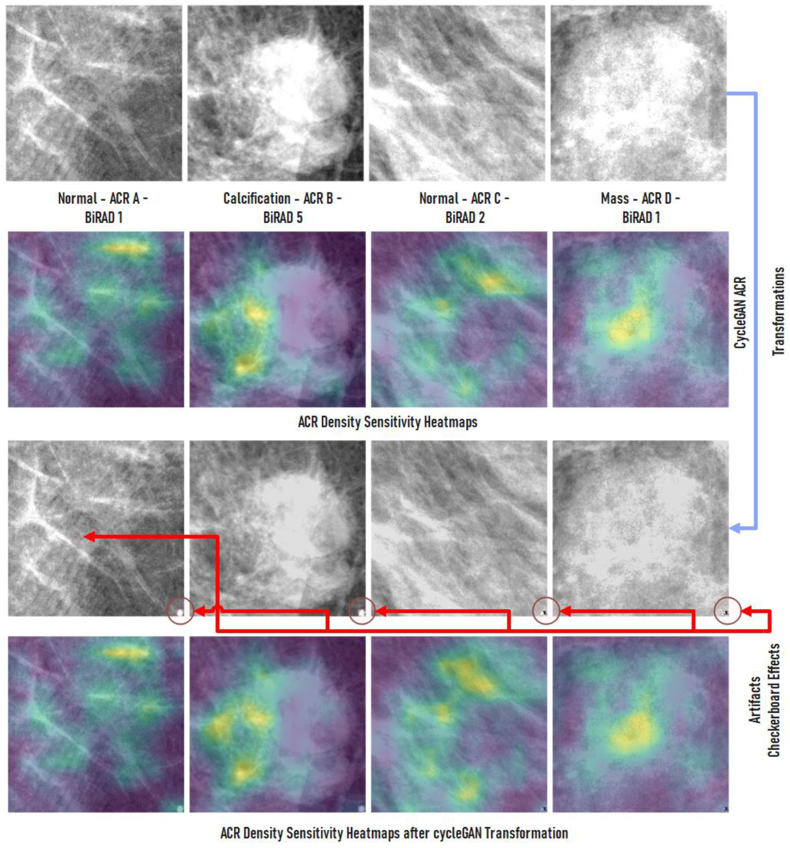
In
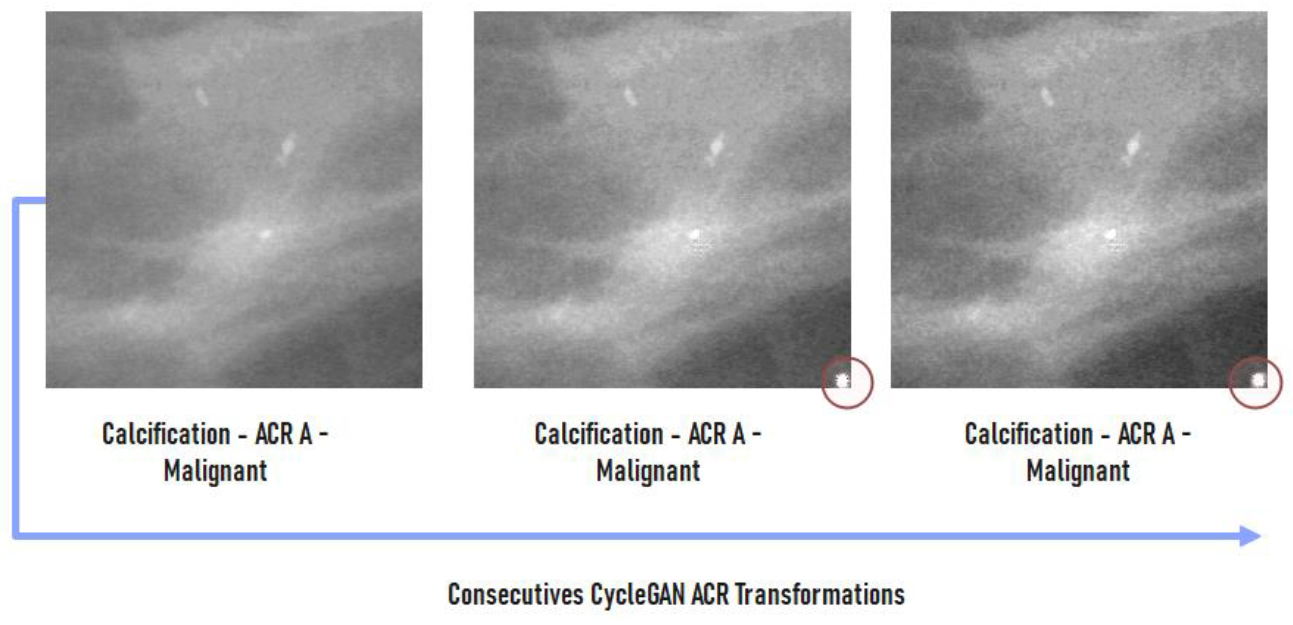
Figure 10, we present some examples of ROI patch transformations to ACR-A density class with the CycleGAN topology along with the changes in the heatmap between the density transformations. For these cases, even after their change in density, the classification of the patch remains unaltered. We have also noted that in a small number of cases, some artifacts appeared in the lower right corner of the resulted patches, but they do not affect the system’s performance in any significant way.
An advantage of the utilized translation model is that consecutive applications of density transformations of the input patches do not alter the ACR classification when the input patch falls in the ACR-A category. In
Figure 10, we depict the results of two successive density transformations of a malignant ACR-A ROI to the ACR-A class via the CycleGAN. It can be seen that the ROI’s density is not altered visually, while the network classifies it again as malignant.
All experiments in this work were carried out on a Linux workstation equipped with an NVIDIA RTX 3090 24 GB, GDDR6X. The deep learning models were all implemented in Python 3.8, in Ubuntu 20.04, with TensorFlow 2.8 and Keras 2.8 API. The CycleGAN model used comes from the original implementations [
41]. Training time for CycleGAN was 25,500 min/epoch for the initially constructed dataset. The model was on average trained for 10 epochs, and the training set was gradually increased via artificially generated images produced by the acGAN model. The augmentation of the datasets was performed via the albumentations library.
3. Experimental Results
To evaluate the performance of the proposed CAD system for each of the previously presented mammographic databases, we have used the precision, recall, accuracy and F1-score metrics as follows:
True positive (TP) represents the number of positive cases that have been correctly classified as positive. True negative (TN) is the number of negative classes that have been correctly classified as negative. False positive (FP) represents the number of negative classes that have been misclassified as the positive class. False negative (FN) represents the number of positive classes that have been misclassified as negative. Typically for each experiment, a confusion matrix was also generated reporting the following cases.
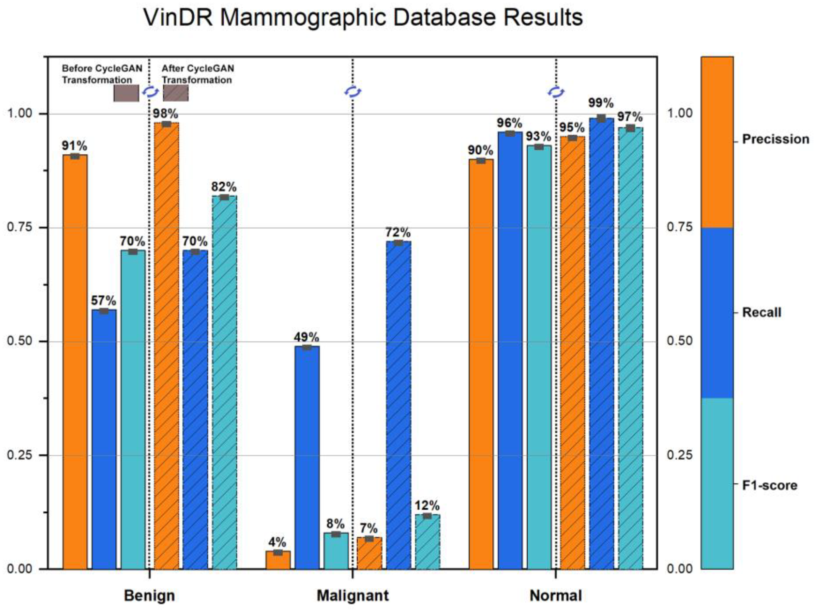
The VinDR-Mammo dataset contains 20,000 total images, of which 988 (4.94%) are malignant, and 5606 (28.03%) are benign. The ACR density distribution is 0.5%, 9.54%, 76.46%, and 13.5% for the four ACR classes, respectively. To compare the overall improvement of the proposed CAD system, all ROI patches are classified before and after changing their density to ACR-A using the CycleGAN network. The performance of the CNN model based on VGG16 before and after utilizing the CycleGAN transformations is depicted in
Figure 11, which shows a significant improvement in the metrics. The recognition results on the left of each dotted line correspond to the initial CNN performance, while the results on the right correspond to the performance after the application of the CycleGAN density transformations. The overall accuracy is dramatically increased from 85% to 91%.
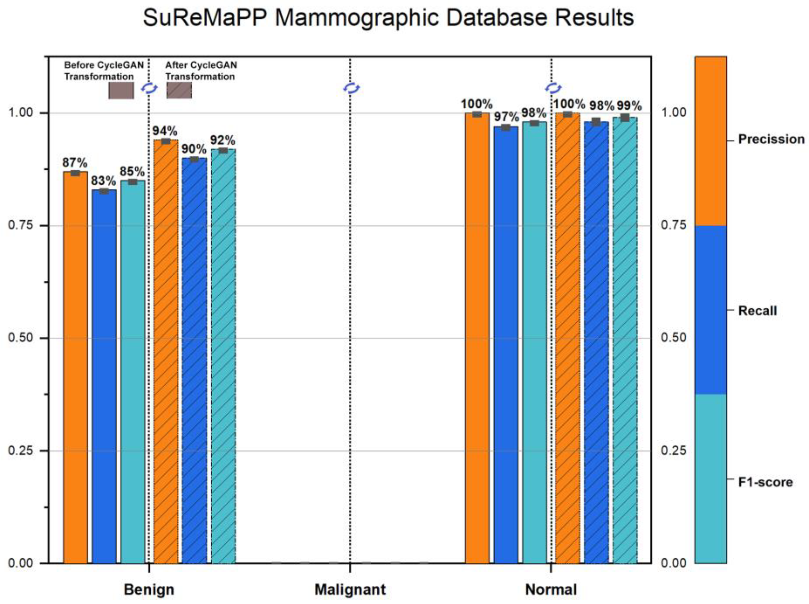
The SuReMaPP dataset contains 343 images, with 0 (0%) malignant and 132 (38.48%) benign cases. The results for the SuReMaPP dataset are shown in
Figure 12. The overall accuracy is further improved from 96% to 98%.
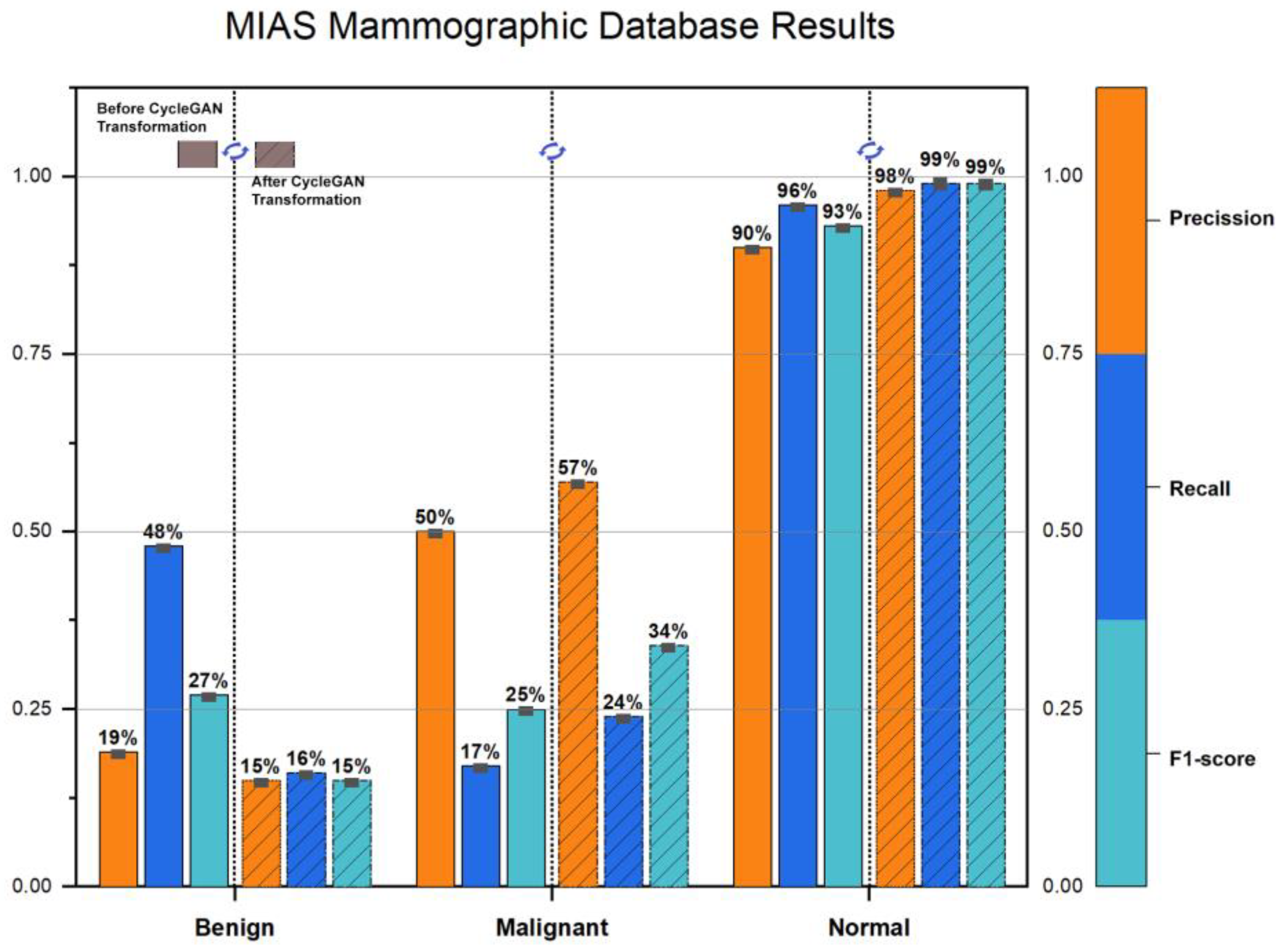
The MIAS dataset contains 322 total images, with 54 (16.77%) malignant and 69 (21.43%) benign cases. The results for the MIAS dataset are shown in
Figure 13. The overall accuracy is increased from 96% to 97%.
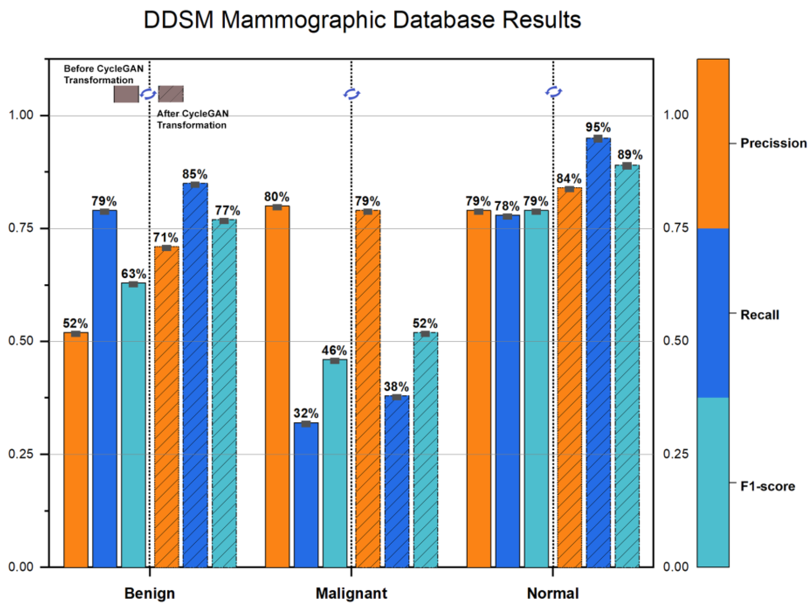
The DDSM (digital database for screening mammography) dataset contains 10,480 images, with 1936 (18.7%) malignant and 2628 (25.4%) benign cases. The results for the DDSM dataset are shown in
Figure 14. The overall accuracy is dramatically improved from 67% to 79%.
For comparison reasons, we report the proposed system’s performance when using the INbreast dataset, which was used in all the relevant CNN/GAN-based topologies for training. The INbreast dataset contains 410 images, with 100 (24.39%) malignant, 243 (59.27%) benign, and 67 (16.34%) normal cases. The percentage of images in each ACR category is 36%, 35%, 22%, and 7%, respectively. In
Table 1, we present the evaluation of the VGG16 classification model (normal–benign–malignant)
For the incorrectly classified ROI patches, after exploiting the CycleGAN model to transform their density to ACR-A class, the classification results are shown in
Table 2.
From the above table, we see an F1-Score of 60%. Only the patches falsely classified as normal–benign–malignant in
Table 1 are processed by the CycleGAN model, which transforms their ACR densities to ACR-A and recalculates the classification outcome. The combination of the data in
Table 1 and
Table 2 give a total classification accuracy for the INbreast dataset of 99.77%.
4. Discussion
Breast tissue density is a known risk factor for cancer development, as women with denser breasts have a higher likelihood of developing cancerous regions compared to women with less dense tissue. However, abnormalities in the breast, whether malignant or benign, can often be concealed by the glandular and connective tissue, making it difficult for both radiologists and computer-assisted diagnosis systems to identify them early or during follow-up screening. Because connective tissue, glandular tissue, and malignancies all appear as white regions on a mammogram, cancerous regions may be hidden by healthy tissue. Our approach considers the density of the examined region of interest (ROI) by attempting to “uncover” and reveal what is masked by the tissue effect.
In this study, we used two types of public screening mammography datasets, film and digital, to demonstrate the effectiveness of our proposed method. It is important to note that our proposed reverse transformation process based on CycleGANs only operates within the breast density mask and applies solely to those ROI patches that are incorrectly classified by classical CNN-based CAD systems as normal, benign, or malignant. Consistent with our experimental findings, the CycleGAN model successfully learned to translate ROI breast density from low to high (and vice versa) while preserving all domain features necessary for accurate type classification.
In the film mammography datasets (MIAS, DDSM), the accuracy improvement is up to 12%, which can be attributed to the CycleGAN model’s ACR reverse transformation process acting as an image enhancement step. However, the image quality of these datasets is inferior to that of fully digital ones (VinDR, SuReMaPP, INbreast), where the accuracy improvement is up to 6% at most, as these mammograms have better quality with no extreme intensity variations. When dealing with datasets acquired with equipment variations in hardware and time, the histogram transfer technique produces a good common reference and makes film mammography usable in mixed CNN-based solutions.
Although CycleGANs often introduce artifacts in the output images (as seen in the lower right corner of patches in
Figure 7 and
Figure 10), this behavior is expected and does not affect the validity of the artificial patches. These artifacts can be resolved with longer training epochs and more unpaired patch samples. In this work, we used 18K total unpaired ACR class patches (9K from class ACR-A, and 9K from classes ACR-B, -C, and -D, both real and artificial ones produced by the acGAN model), which took approximately six months on an RTX 3090/24 GB-based system for producing valid ACR class patches. The ACR heatmaps demonstrate that the transformed patches’ density changes do not affect the patch’s classification into the appropriate ACR class, providing macroscopic evidence of the process’s ground truth.
We did not optimize the CNNs/GAN topologies in terms of hyperparameters, but we attempted to keep our system’s design relatively simple while enhancing its accuracy performance. More sophisticated and precise models can be deployed. Furthermore, our task, which involves transforming the ACR density of the examined ROI to reveal underlying findings, works particularly well for ACR density classes B and C, which account for 80% of all female breast cancer cases. For ACR-A, the density transformation back to the same class A contributes very little, as expected. Similarly, findings in class D density ROIs are much harder to identify, and the density transformation process should be augmented by extra information (such as BI-RAD characterization) for better diagnostic outcomes.
5. Conclusions
Our study presents a new computer-aided diagnosis (CAD) system for breast cancer that can classify suspicious regions of mammograms into three categories: normal, benign, and malignant. Our aim is to improve the accuracy of this classification by taking into account the density of the patient’s breast tissue. Dense breasts are more likely to have invasive ductal carcinoma due to the increased amount of glandular tissue, which can make it harder to detect abnormalities. Our proposed CAD system solves the problem of “masking” in mammograms, where dense breast tissue can hide abnormalities. We achieve this by using a process that reverses the effects of breast density on mammograms.
As we hypothesized, the CycleGAN models not only learned how to translate from low-to-high breast density but also preserved the domain characteristics during translation. However, the present study is not without limitations. One limitation of our work involves the availability of healthy ACR-D mammograms to train the generative models. There are not many annotated datasets publicly available that are fully digital, so one must resort to a closed set of mammograms. Another limitation is the imbalanced nature of the problem; the ratio between the different ACR classes is by no means equally distributed. In our approach, this was partially resolved by using image manipulation methods (i.e., GANs) that produced artificially patched images via domain adaptation. However, it is known that this process does not extend the feature space of the problem but rather produces structurally similar images, which, in many cases, result in overfitting. Although the sophisticated mathematics underlying deep learning training algorithms is conceptually understandable, their architectures are more of a “black box” paradigm. In the case of the breast density CycleGAN, one must comprehend the learned mapping via post hoc explainability [
42]. The post hoc explanation is a task that will be performed in future work. We also plan to conduct further testing of our proposed system using real clinical images and interpret the transformations performed by the CycleGAN with the assistance of a team of radiologists.
Although more data are needed to fully examine the extent of this reverse process, in all datasets that we tested, the overall percentage of successful recognition for normal/benign/malignant ROIs was improved significantly. In future work, we plan to expand this method to the whole breast region, by using more advanced GANs and CNNs that can analyze the relationships between neighboring areas. Our approach could help doctors and radiologists identify suspicious regions and plan treatments at an early stage, potentially avoiding consequences and treatment difficulties.
Author Contributions
Conceptualization, D.A., G.A. and A.K.; methodology, A.K.; software, D.A., G.A. and I.C.; validation, G.A. and I.C.; formal analysis, D.A. and A.K.; investigation, D.A., G.A. and I.C.; resources, G.A. and I.C.; data curation, D.A. and G.A.; writing—original draft preparation, D.A. and A.K.; writing—review and editing, D.A. and A.K.; visualization, G.A. and I.C.; supervision, A.K. All authors have read and agreed to the published version of the manuscript.
Funding
This research received no external funding.
Institutional Review Board Statement
There are no ethical implications on public dataset.
Informed Consent Statement
There are no ethical implications on the public dataset.
Data Availability Statement
All the datasets used are publicly available.
Conflicts of Interest
The authors declare no conflict of interest.
References
- Ali, E.A.; Raafat, M. Relationship of mammographic densities to breast cancer risk. Egypt. J. Radiol. Nucl. Med. 2021, 52, 129. [Google Scholar] [CrossRef]
- Ciritsis, A.; Rossi, C.; De Martini, I.; Eberhard, M.; Marcon, M.; Becker, A.S.; Berger, N.; Boss, A. Determination of mammographic breast density using a deep convolutional neural network. Br. J. Radiol. 2018, 92, 20180691. [Google Scholar] [CrossRef] [PubMed]
- Gemici, A.A.; Bayram, E.; Hocaoglu, E.; Inci, E. Comparison of breast density assessments according to BI-RADS 4th and 5th editions and experience level. Acta Radiol. Open 2020, 9, 2058460120937381. [Google Scholar] [CrossRef]
- Weigel, S.; Heindel, W.; Heidrich, J.; Hense, H.-W.; Heidinger, O. Digital mammography screening: Sensitivity of the programme dependent on breast density. Eur. Radiol. 2016, 27, 2744–2751. [Google Scholar] [CrossRef] [PubMed]
- Wanders, J.O.P.; Holland, K.; Veldhuis, W.B.; Mann, R.M.; Pijnappel, R.M.; Peeters, P.H.M.; van Gils, C.H.; Karssemeijer, N. Volumetric breast density affects performance of digital screening mammography. Breast Cancer Res. Treat. 2016, 162, 95–103. [Google Scholar] [CrossRef]
- Sexauer, R.; Hejduk, P.; Borkowski, K.; Ruppert, C.; Weikert, T.; Dellas, S.; Schmidt, N. Diagnostic accuracy of automated ACR BI-RADS breast density classification using deep convolutional neural networks. Eur. Radiol. 2023, 1–8. [Google Scholar] [CrossRef]
- Rao, V.M.; Levin, D.C.; Parker, L.; Cavanaugh, B.; Frangos, A.J.; Sunshine, J.H. How Widely Is Computer-Aided Detection Used in Screening and Diagnostic Mammography? J. Am. Coll. Radiol. 2010, 7, 802–805. [Google Scholar] [CrossRef]
- Chan, H.-P.; Samala, R.K.; Hadjiiski, L.M. CAD and AI for breast cancer—Recent development and challenges. Br. J. Radiol. 2020, 93, 20190580. [Google Scholar] [CrossRef]
- Hassan, N.M.; Hamad, S.; Mahar, K. Mammogram breast cancer CAD systems for mass detection and classification: A review. Multimed. Tools Appl. 2022, 81, 20043–20075. [Google Scholar] [CrossRef]
- Lee, J.; Nishikawa, R.M. Analyzing GAN artifacts for simulating mammograms: Application towards finding mammographically-occult cancer. In Proceedings of the Medical Imaging 2022: Computer-Aided Diagnosis, San Diego, CA, USA, 20 February–28 March 2022; Volume 120330. [Google Scholar] [CrossRef]
- Korkinof, D.; Rijken, T.; O’Neill, M.; Yearsley, J.; Harvey, H.; Glocker, B. High-resolution mammogram synthesis using progressive generative adversarial networks. arXiv 2019, arXiv:1807.03401. [Google Scholar]
- Yamazaki, A.; Ishida, T. Two-View Mammogram Synthesis from Single-View Data Using Generative Adversarial Networks. Appl. Sci. 2022, 12, 12206. [Google Scholar] [CrossRef]
- Desai, S.D.; Giraddi, S.; Verma, N.; Gupta, P.; Ramya, S. Breast Cancer Detection Using GAN for Limited Labeled Dataset. In Proceedings of the 12th International Conference on Computational Intelligence and Communication Networks (CICN), Bhimtal, India, 25–26 September 2020; pp. 34–39. [Google Scholar] [CrossRef]
- Oyelade, O.N.; Ezugwu, A.E.; Almutairi, M.S.; Saha, A.K.; Abualigah, L.; Chiroma, H. A generative adversarial network for synthetization of regions of interest based on digital mammograms. Sci. Rep. 2022, 12, 6166. [Google Scholar] [CrossRef] [PubMed]
- El-Ghoussani, A.; Rodríguez-Salas, D.; Seuret, M.; Maier, A. GAN-based Augmentation of Mammograms to Improve Breast Lesion Detection. In Bildverarbeitung für die Medizin 2022; Maier-Hein, K., Deserno, T.M., Handels, H., Maier, A., Palm, C., Tolxdorff, T., Eds.; Informatik aktuell; Springer: Wiesbaden, Germany, 2022. [Google Scholar] [CrossRef]
- Osuala, R.; Kushibar, K.; Garrucho, L.; Linardos, A.; Szafranowska, Z.; Klein, S.; Glocker, B.; Diaz, O.; Lekadir, K. Data synthesis and adversarial networks: A review and meta-analysis in cancer imaging. Med. Image Anal. 2023, 84, 1–64. [Google Scholar] [CrossRef]
- Pham, H.H.; Trung, H.N.; Nguyen, H.Q. VinDr-Mammo: A large-scale benchmark dataset for computer-aided detection and diagnosis in full-field digital mammography. PhysioNet 2022. [Google Scholar] [CrossRef]
- Bruno, A.; Ardizzone, E.; Vitabile, S.; Midiri, M. A Novel Solution Based on Scale Invariant Feature Transform Descriptors and Deep Learning for the Detection of Suspicious Regions in Mammogram Images. J. Med. Signals Sens. 2020, 10, 158–173. [Google Scholar] [CrossRef]
- Suckling, J.; Parker, J.; Dance, D.; Astley, S.; Hutt, I.; Boggis, C.; Ricketts, I.; Stamatakis, E.; Cerneaz, N.; Kok, S.; et al. Mammographic Image Analysis Society; Apollo—University of Cambridge: Cambridge, UK, 2015. [Google Scholar]
- Heath, M.; Bowyer, K.; Kopans, D.; Kegelmeyer, P.; Moore, R.; Chang, K.; Munishkumaran, S. Current Status of the Digital Database for Screening Mammography. In Digital Mammography; Karssemeijer, N., Thijssen, M., Hendriks, J., van Erning, L., Eds.; Springer: Dordrecht, The Netherlands, 1998; pp. 457–460. [Google Scholar] [CrossRef]
- Archive, C.I. Curated Breast Imaging Digital Database for Screening Mammography (DDSM). 2021. Available online: https://wiki.cancerimagingarchive.net/display/Public/CBIS-DDSM (accessed on 31 March 2023).
- University of South Florida. Digital Database for Screening Mammography (DDSM). 2021. Available online: http://www.eng.usf.edu/cvprg/Mammography/Database.html (accessed on 31 March 2023).
- Moreira, I.C.; Amaral, I.; Domingues, I.; Cardoso, A.; Cardoso, M.J.; Cardoso, J.S. INbreast: Toward a Full-field Digital Mammographic Database. Acad. Radiol. 2012, 19, 236–248. [Google Scholar] [CrossRef] [PubMed]
- Erkan, U.; Gökrem, L.; Enginoğlu, S. Different applied median filter in salt and pepper noise. Comput. Electr. Eng. 2018, 70, 789–798. [Google Scholar] [CrossRef]
- Sun, X.; Shi, L.; Luo, Y.; Yang, W.; Li, H.; Liang, P.; Li, K.; Mok, V.C.T.; Chu, W.C.W.; Wang, D. Histogram-based normalization technique on human brain magnetic resonance images from different acquisitions. Biomed. Eng. Online 2015, 14, 73. [Google Scholar] [CrossRef] [PubMed]
- Qiao, T.; Ren, J.; Wang, Z.; Zabalza, J.; Sun, M.; Zhao, H.; Li, S.; Benediktsson, J.A.; Dai, Q.; Marshall, S. Effective Denoising and Classification of Hyperspectral Images Using Curvelet Transform and Singular Spectrum Analysis. IEEE Trans. Geosci. Remote. Sens. 2016, 55, 119–133. [Google Scholar] [CrossRef]
- Pizer, S.M.; Amburn, E.P.; Austin, J.D.; Cromartie, R.; Geselowitz, A.; Greer, T.; ter Haar Romeny, B.; Zimmerman, J.B.; Zuiderveld, K. Adaptive histogram equalization and its variations. Comput. Vis. Graph. Image Process. 1987, 39, 355–368. [Google Scholar] [CrossRef]
- Pisano, E.D.; Zong, S.; Hemminger, B.M.; DeLuca, M.; Johnston, R.E.; Muller, K.; Braeuning, M.P.; Pizer, S.M. Contrast limited adaptive histogram equalization image processing to improve the detection of simulated spiculations in dense mammograms. J. Digit. Imaging 1998, 11, 193–200. [Google Scholar] [CrossRef] [PubMed]
- Sahakyan, A.; Sarukhanyan, H. Segmentation of the breast region in digital mammograms and detection of masses. Int. J. Adv. Comput. Sci. Appl. 2012, 3, 102–105. [Google Scholar] [CrossRef]
- Ronneberger, O.; Fischer, P.; Brox, T. U-Net: Convolutional networks for biomedical image segmentation. In Medical Image Computing and Computer-Assisted Intervention 2015; Navab, N., Hornegger, J., Wells, W.M., Frangi, A.F., Eds.; Springer: Cham, Switzerland, 2015; pp. 234–241. [Google Scholar] [CrossRef]
- Han, J.; Zhang, D.; Hu, X.; Guo, L.; Ren, J.; Wu, F. Background Prior-Based Salient Object Detection via Deep Reconstruction Residual. IEEE Trans. Circuits Syst. Video Technol. 2014, 25, 1309–1321. [Google Scholar] [CrossRef]
- Zabalza, J.; Ren, J.; Zheng, J.; Zhao, H.; Qing, C.; Yang, Z.; Du, P.; Marshall, S. Corrigendum to ‘Novel segmented stacked autoencoder for effective dimensionality reduction and feature extraction in hyperspectral imaging’. Neurocomputing 2016, 214, 1062. [Google Scholar] [CrossRef]
- LeCun, Y.; Kavukcuoglu, K.; Farabet, C. Convolutional networks and applications in vision. In Proceedings of the 2010 IEEE International Symposium on Circuits and Systems: Nano-Bio Circuit Fabrics and Systems, Paris, France, 30 May–2 June 2010; pp. 253–256. [Google Scholar]
- Mohamed, A.A.; Luo, Y.; Peng, H.; Jankowitz, R.C.; Wu, S. Understanding Clinical Mammographic Breast Density Assessment: A Deep Learning Perspective. J. Digit. Imaging 2017, 31, 387–392. [Google Scholar] [CrossRef] [PubMed]
- Peng, X.; Tang, Z.; Yang, F.; Feris, R.S.; Metaxas, D. Jointly optimize data augmentation and network training: Adversarial data augmentation in human pose estimation. In Proceedings of the IEEE Conference on Computer Vision and Pattern Recognition (CVPR), Salt Lake City, UT, USA, 18–23 June 2018. [Google Scholar]
- Yu, A.; Grauman, K. Semantic Jitter: Dense Supervision for Visual Comparisons via Synthetic Images. In Proceedings of the IEEE International Conference on Computer Vision (ICCV), Venice, Italy, 22–29 October 2017. [Google Scholar]
- Wang, X.; Shrivastava, A.; Gupta, A. A-Fast-RCNN: Hard Positive Generation via Adversary for Object Detection. arXiv 2017, arXiv:1704.03414. [Google Scholar]
- Wang, Y.X.; Girshick, R.; Hebert, M.; Hariharan, B. Hariharan, Low-shot learning from imaginary data. arXiv 2018, arXiv:1801.05401. [Google Scholar]
- Antoniou, A.; Storkey, A.; Edwards, H. Augmenting Image Classifiers Using Data Augmentation Generative Adversarial Networks. In Proceedings of the International Conference on Artificial Neural Networks, Bratislava, Slovakia, 15–18 September 2018; pp. 594–603. [Google Scholar] [CrossRef]
- Zhu, J.; Park, T.; Isola, P.; Efros, A. Unpaired Image-to-Image Translation Using Cycle-Consistent Adversarial Networks. In Proceedings of the IEEE International Conference on Computer Vision (ICCV), Venice, Italy, 22–29 October 2017; pp. 2242–2251. [Google Scholar]
- Johnson, J.; Alahi, A.; Fei-Fei, L. Perceptual losses for real-time style transfer and super-resolution. In Proceedings of the European Conference on Computer Vision, Amsterdam, The Netherland, 8–16 October 2016; Springer: Berlin/Heidelberg, Germany, 2016; pp. 694–711. [Google Scholar]
- Dhar, T.; Dey, N.; Borra, S.; Sherratt, R.S. Challenges of Deep Learning in Medical Image Analysis—Improving Explainability and Trust. IEEE Trans. Technol. Soc. 2023, 4, 68–75. [Google Scholar] [CrossRef]
Figure 1.
Overview of a typical breast. (Adapted from here. Original image by Patrick J. Lynch, medical illustrator; C. Carl Jaffe, MD, cardiologist, is licensed under the Creative Commons Attribution 2.5 Generic license).
Figure 1.
Overview of a typical breast. (Adapted from here. Original image by Patrick J. Lynch, medical illustrator; C. Carl Jaffe, MD, cardiologist, is licensed under the Creative Commons Attribution 2.5 Generic license).
Figure 2.
CAD system pipeline.
Figure 2.
CAD system pipeline.
Figure 3.
The architecture of the U-NET model with an input sample size of 572 × 572 pixels as input. The training procedure was conducted using the INbreast database.
Figure 3.
The architecture of the U-NET model with an input sample size of 572 × 572 pixels as input. The training procedure was conducted using the INbreast database.
Figure 4.
Examples of artificially generated images of the normal, malignant and benign classes using the GAN-NMB network. (Note that checkerboard effects and artifacts are present.)
Figure 4.
Examples of artificially generated images of the normal, malignant and benign classes using the GAN-NMB network. (Note that checkerboard effects and artifacts are present.)
Figure 5.
Examples of artificially generated images of ACR-A, ACR-B, ACR-C, and ACR-D classes using the GAN-ACR network. (Note that checkerboard effects and artifacts are present.)
Figure 5.
Examples of artificially generated images of ACR-A, ACR-B, ACR-C, and ACR-D classes using the GAN-ACR network. (Note that checkerboard effects and artifacts are present.)
Figure 6.
The CycleGAN Overview: Domain-A has patches with ACR-A density, and Domain-B has patches with ACR-B, -C and -D density.
Figure 6.
The CycleGAN Overview: Domain-A has patches with ACR-A density, and Domain-B has patches with ACR-B, -C and -D density.
Figure 7.
Transformation of ACR-B, -C, and -D to the ACR-A category.
Figure 7.
Transformation of ACR-B, -C, and -D to the ACR-A category.
Figure 8.
Transformation of ACR-A to ACR-D and ACR-C category.
Figure 8.
Transformation of ACR-A to ACR-D and ACR-C category.
Figure 9.
Consecutive ACR density transformations via CycleGAN (two times transformations of an ACR-A ROI).
Figure 9.
Consecutive ACR density transformations via CycleGAN (two times transformations of an ACR-A ROI).
Figure 10.
Illustration of ACR heatmaps before and after CycleGAN transformations. ACR density sensitivity remains almost the same.
Figure 10.
Illustration of ACR heatmaps before and after CycleGAN transformations. ACR density sensitivity remains almost the same.
Figure 11.
CNN performance before and after CycleGAN transformations—VinDR—Mammographic Database.
Figure 11.
CNN performance before and after CycleGAN transformations—VinDR—Mammographic Database.
Figure 12.
CNN performance before and after CycleGAN transformations—SuReMaPP—Mammographic Database.
Figure 12.
CNN performance before and after CycleGAN transformations—SuReMaPP—Mammographic Database.
Figure 13.
CNN performance before and after CycleGAN transformations—MIAS—Mammographic Database.
Figure 13.
CNN performance before and after CycleGAN transformations—MIAS—Mammographic Database.
Figure 14.
CNN performance before and after CycleGAN transformations—DDSM—Mammographic Database.
Figure 14.
CNN performance before and after CycleGAN transformations—DDSM—Mammographic Database.
Table 1.
CNN performance before CycleGAN—INbreast. In the first part, the confusion matrix shows the number of misclassified patches before any transformation of the tissue density.
Table 1.
CNN performance before CycleGAN—INbreast. In the first part, the confusion matrix shows the number of misclassified patches before any transformation of the tissue density.
| | Benign | Malignant | Normal | Precision | Recall | F1-Score | Support |
|---|
| Benign | 355,029 | 1035 | 2629 | 0.99 | 0.99 | 0.99 | 358,693 |
| Malignant | 1875 | 845,068 | 4125 | 1.00 | 0.99 | 0.99 | 851,068 |
| Normal | 1747 | 2109 | 1,134,459 | 0.99 | 1.00 | 1.00 | 1,138,315 |
| Accuracy | | | | | | 0.99 | 2,348,076 |
| Macro avg. | | | | 0.99 | 0.99 | 0.99 | 2,348,076 |
| Weighted avg. | | | | 0.53 | 0.99 | 0.99 | 2,348,076 |
Table 2.
CNN accuracy performance for the falsely recognized patches of
Table 1, after CycleGAN patches density transformation.
Table 2.
CNN accuracy performance for the falsely recognized patches of
Table 1, after CycleGAN patches density transformation.
| | Benign | Malignant | Normal | Precision | Recall | F1-Score | Support |
|---|
| Benign | 2690 | 398 | 576 | 0.59 | 0.73 | 0.66 | 3664 |
| Malignant | 1358 | 2486 | 2156 | 0.74 | 0.41 | 0.53 | 6000 |
| Normal | 476 | 472 | 2908 | 0.52 | 0.75 | 0.61 | 3856 |
| Accuracy | | | | | | 0.60 | 13,520 |
| Macro avg. | | | | 0.62 | 0.63 | 0.60 | 13,520 |
| Weighted avg. | | | | 0.59 | 0.73 | 0.66 | 3664 |
| Disclaimer/Publisher’s Note: The statements, opinions and data contained in all publications are solely those of the individual author(s) and contributor(s) and not of MDPI and/or the editor(s). MDPI and/or the editor(s) disclaim responsibility for any injury to people or property resulting from any ideas, methods, instructions or products referred to in the content. |
© 2023 by the authors. Licensee MDPI, Basel, Switzerland. This article is an open access article distributed under the terms and conditions of the Creative Commons Attribution (CC BY) license (https://creativecommons.org/licenses/by/4.0/).


 ,
, 


