Experimental Prediction Method of Free-Field Sound Emissions Using the Boundary Element Method and Laser Scanning Vibrometry

Abstract

Acoustic emissions play a major role in the usability of many product categories. Therefore, mitigating the emitted sound directly at the source is paramount to improve usability and customer satisfaction. To reliably predict acoustic emissions, numerical methods such as the boundary element method (BEM) are employed, which allow for predicting, e.g., the acoustic emission into the free field. BEM algorithms need appropriate boundary conditions to couple the sound field with the structural motion of the vibrating body. In this contribution, firstly, an interpolation scheme is presented, which allows for appropriate interpolation of arbitrary velocity data to the computational grid of the BEM. Secondly, the free-field Helmholtz problem is solved with the open-source BEM software framework NiHu. The forward coupling between the device of interest and BEM is based on the surface normal velocities (i.e., a Neumann boundary condition). The BEM simulation results are validated using a previously established aeroacoustic benchmark problem. Furthermore, an application to a medical device (knee prosthesis frame) is presented. Furthermore, the radiated sound power is evaluated and contextualized with other low-cost approximations. Regarding the validation example, very good agreements are achieved between the measurements and BEM results, with a mean effective pressure level error of $0.63$ dB averaged across three microphone positions. Applying the workflow to a knee prosthesis frame, the simulation is capable of predicting the acoustic radiation to four microphone positions with a mean effective pressure level error of $1.52$ dB.

1. Introduction

Sound emission quantification of complex solid mechanical systems in engineering applications, ranging from medical applications [1], loudspeakers [2], automotive [3,4,5,6], railway [7], and aerospace industries [8,9,10] to decision-making in architectural acoustics (e.g., placement of a heat pump), is essential for their improvement towards customer satisfaction. Specifically, the identification and evaluation of sound emissions from a knee prosthesis constitute a major part of the development of next-generation prostheses. The noise emissions have multiple negative effects on both the user and the user’s environment [11]. In particular, the boundary element method (BEM) can be efficiently used to simulate sound propagation based on the surface vibration velocity [12]. On the one hand, the mechanical surface velocity may be computed by the structural finite element method (FEM) applied to the solid mechanical system [13]. On the other hand, the normal surface vibration velocity data can be measured using laser-doppler scanning vibrometry (LSV). Over the years, BEM has become a standard procedure for computing the acoustic free-field propagation efficiently [14]. Various improvements have lead to fast simulation prediction methods in the time and time-harmonic case for the linear acoustic field (e.g., fast multipole methods [15]) or utilizing model order reduction [16]. Based on these improvements, BEM has become a standard method for radiating free-field sound into far distances in the mid-frequency range [17].

In the context of the article, the surface velocity is either computed using an FEM model in combination with openCFS (https://opencfs.org/(accessed on 23 November 2023)) [18] or determined experimentally. While FEM simulations capture the mechanical response of the structure under various loads regarding applied modeling simplifications of joints, bearings, connections, material, and geometry, the measured velocity captures the real-world surface velocity response, typically with a comparably low spatial resolution of the surface velocity signal. Based on the data and the Helmholtz equation, BEM is used to predict the acoustic emissions at certain microphone locations [19]. The aim of this paper is to establish a workflow for transforming the surface velocity information into information about the acoustic sound emissions through BEM simulation, and providing validation for multiple test cases. The open source BEM software NiHu (https://last.hit.bme.hu/nihu (accessed on 23 November 2023)) [20] was verified previously by several test cases. In the first step focusing on the automotive industry, the FEM-BEM method was verified and compared with an existing acoustic simulation of a confined flow-sound prediction using the FEM method [21]. This example shows the accuracy of the workflow for a simple, realistic application. Additionally, the influence of low surface resolution was investigated systematically by virtual coarsening of the measurement grid to imitate points of missing surface information.

Regarding this verification example, the method was finally applied to validate the acoustic emissions of a medical knee prosthesis frame under specific test conditions. Acoustic microphone measurements in an anechoic chamber validated the predicted sound emissions. The numerically obtained sound power was compared to a low-cost sound power estimate presented in [22]. In conclusion, the results show very promising sound prediction capabilities, with a mean error of the effective pressure level, as defined in Section 3.2.3 (averaged across four microphone positions) of $1.52$ dB.

The rest of the paper is organized as follows. In Section 2, the data acquisition using an LSV and the successive interpolation algorithm are described. Furthermore, BEM and its implementation in the software framework used are presented. Section 3 describes the verification and validation of the interpolation scheme and the BEM solver. In Section 4, an application of the workflow to an industrial use case, i.e., sound radiation of a clinically applied knee prosthesis, is presented. Finally, Section 5 discusses the main findings.

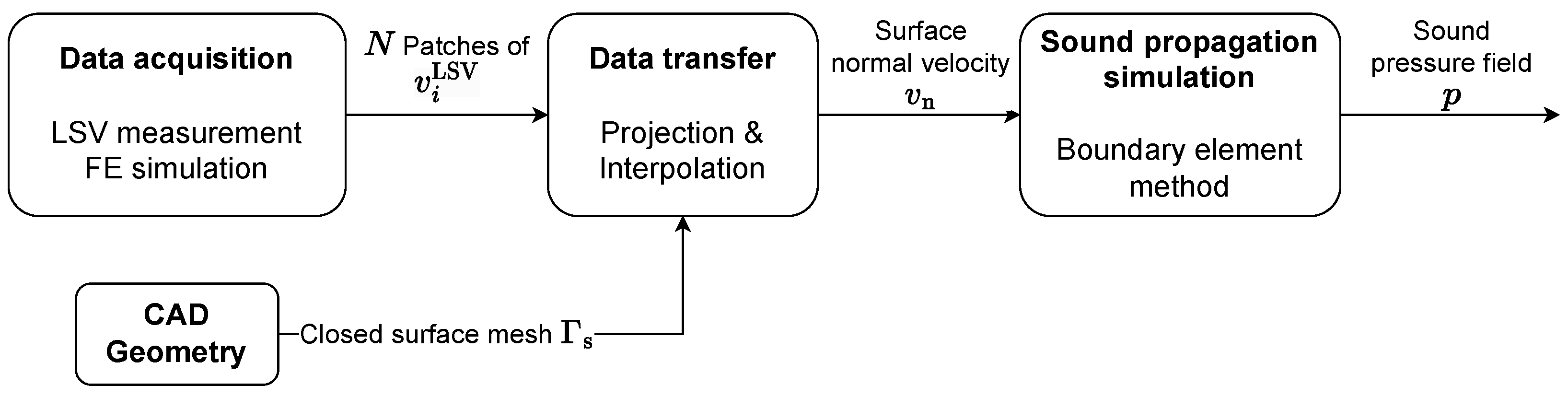
2. Methods

In most technical applications, sound radiation can be modeled by applying forward coupling of the structural vibration domain to the acoustic propagation domain, as depicted in Figure 1. Consequently, any effect of the incident pressure field on the structure is neglected [2,3]. The forward coupling is achieved by prescribing the normal component of the acoustic particle velocity $v_n$ to the corresponding surface velocity of the structure, i.e., applying an inhomogeneous Neumann boundary condition for the wave equation (see Section 2.2). For simple structures, the surface velocity of the structure can be obtained, e.g., by FE simulation of the structural dynamics. This workflow is described in Section 3.2 using the FE solver openCFS. However, in industrial applications, the high number of contact points and joints in complex assemblies or the use of compound materials in light-weight applications can make simulations of the mechanical structure infeasible with reasonable effort. Therefore, when applying the proposed method to an industrial use case, measurement data from LSV measurements are used instead as an input for the sound prediction model, as demonstrated in Section 4.

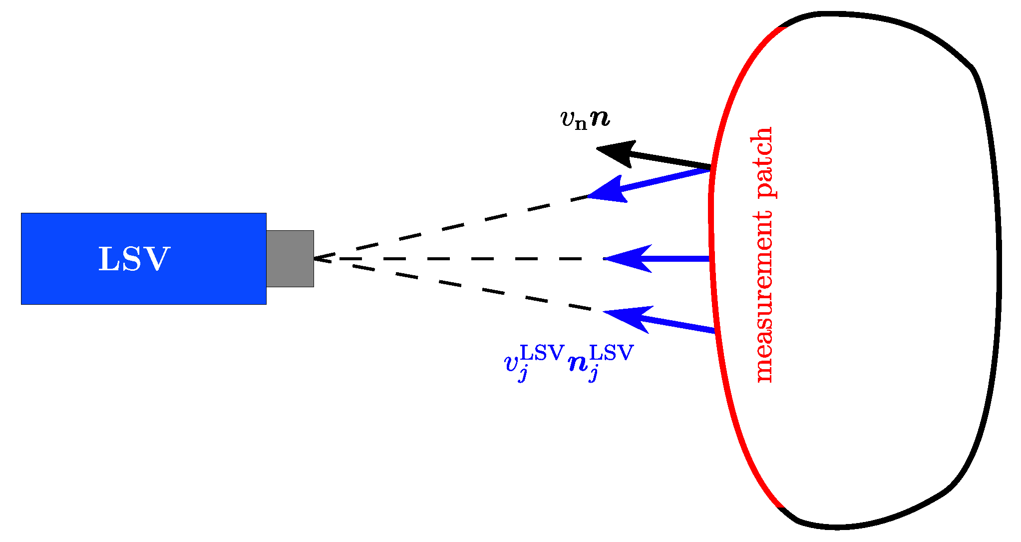
2.1. Data Acquisition

The surface normal velocity, required as a boundary condition for the acoustic propagation model (see Section 2.2), can be obtained efficiently by experiments using an LSV, as depicted schematically in Figure 2. Laser vibrometry is based on the interference of a reference laser beam with a laser beam reflected by the surface, which is frequency modulated based on the Doppler effect [23]. Thereby, the surface velocity in the laser direction $v_j^{\mathrm{LSV}}=\mathit{v}·{\mathit{n}}_j^{\mathrm{LSV}}$ can be measured, where ${\mathit{n}}_j^{\mathrm{LSV}}$ denotes the unit vector in the laser direction and the index j the index of the measured surface location. Consequently, the three-dimensional velocity vector $\mathit{v}$ can be reconstructed from three independent excitation-synchronized measurements using unique laser directions to guarantee observability. When dealing with nearly flat surfaces, it can be sufficient to position the laser scanning head in the dominant direction of overall normal motion and use this velocity component to approximate the normal velocity $v_{\mathrm{n}}$.

Laser scanning vibrometry allows for the subsequent measurement of an array of points on the surface, such that the vibrometer has to be repositioned a limited number of times to obtain data on all relevant areas. This results in N patches of measurement data. Data on these measured patches must be transferred to a closed (and most often refined) surface mesh used for the acoustic propagation simulation (see Section 2.3). This data transfer comes with the following challenges:

• Imperfect representation of the geometry by the measured surface patch;
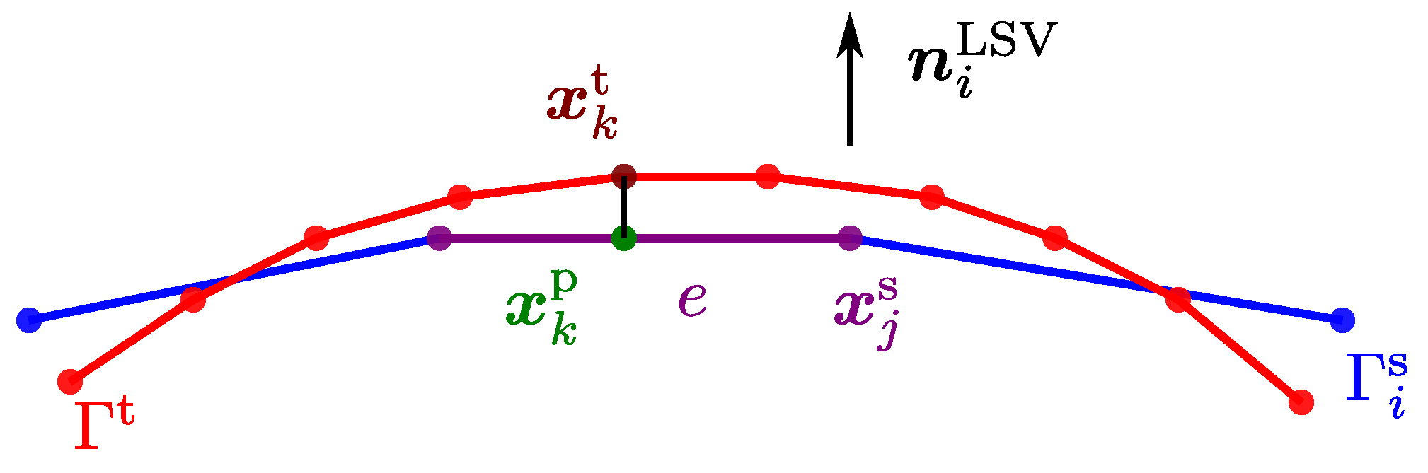
• Spatial up-sampling of coarsely distributed measurement data; 
• Overlapping data patches.

To overcome these challenges, a two-staged data transfer process is proposed, consisting of a projection and an interpolation step, which is combined into a linear transformation ${\mathit{T}}_i$ for each measurement patch i. In the following, the mesh of the closed geometry used for the simulation is called target ${\Gamma }^{\mathrm{t}}$, and patch i containing the measurement data is called source ${\Gamma }_i^{\mathrm{s}}$. The algorithm to obtain the transformation matrix ${\mathit{T}}_i$ is shown in Algorithm 1. It is described in the following: For any given point ${\mathit{x}}_k^{\mathrm{t}}$ on the target mesh, the location is projected in the measurement direction onto the source mesh. For simplicity, the measurement direction used for the projection is averaged over all points in a patch, resulting in a mean direction ${\mathit{n}}_i^{\mathrm{LSV}}$. Suppose the surface has a complex shape but is sufficiently smooth (or the edges are treated separately). In that case, the projection direction can also be obtained by averaging the normal vectors of the neighboring elements for each point on ${\Gamma }^{\mathrm{t}}$. Next, linear shape functions $N_j\left(\mathit{x}\right)$ are evaluated for the projected point ${\mathit{x}}_k^{\mathrm{p}}$ in the according element e. In this context, the (linear) shape function evaluation can also be used to check whether the projected point is inside any element. Finally, the shape function values are used as transformation coefficients corresponding to the source grid point indices and the index of the target point.

$${\mathit{T}}_i=\left[T_{j,k}\right]=\left[N_j\left({\mathit{x}}_k^{\mathrm{p}}\right)\right]\forall j\in e\in {\Gamma }^{\mathrm{s}}\wedge \forall k\in {\Gamma }^{\mathrm{t}}.$$

(1)

Algorithm 1 Data transformation matrix

${\mathit{n}}_i^{\mathrm{LSV}}\leftarrow \mathtt{mean}\left({\mathit{n}}_j^{\mathrm{LSV}}\right)$            ▹ Compute projection direction for ${\mathit{x}}_k^{\mathrm{t}}\in {\Gamma }^{\mathrm{t}}$ do                ▹ Loop over nodes in target grid     for ${\mathit{x}}_j^{\mathrm{s}},{\mathit{x}}_e\in {\Gamma }^{\mathrm{s}}$ do         ▹ Loop over nodes / elements in source grid         if $\left|\right|{\mathit{x}}_k^{\mathrm{t}}-{\mathit{x}}_e\left|\right|<\mathtt{maxDist}$ then      ▹ Skip points that are too far apart            ${\mathit{x}}_k^{\mathrm{p}}\leftarrow \mathtt{projectPoint}\left({\mathit{n}}_i^{\mathrm{LSV}}\right)$          ▹ Project point onto source grid            if ${\mathit{x}}_k^{\mathrm{p}}\in e$ then     ▹ Check if projected point is inside the element                $N_j\leftarrow \mathtt{evalShapeFunction}\left({\mathit{x}}_k^{\mathrm{p}}\right) \forall j\in e$ ▹ Compute interpolation weights                $T_{j,k}\leftarrow N_j$            end if         end if     end for end for

A sketch of Algorithm 1 for a two-dimensional problem is provided in Figure 3. It depicts an arbitrary source and target surface mesh in two dimensions, both comprised of discrete points. The process of data transformation is illustrated, where the location from the target mesh geometry ${\mathit{x}}_k^{\mathrm{t}}$ is projected onto the source mesh geometry ${\Gamma }_i^{\mathrm{s}}$ using the mean measurement direction ${{\mathit{n}}_{\mathit{I}}}^{\mathrm{LSV}}$ as projection direction. The black line from the target mesh ${\Gamma }_s^{\mathrm{t}}$ in red to the source mesh ${\Gamma }_s^{\mathrm{s}}$ in blue represents the projection step. It should be noted that the transfer direction of data values is opposite to the projection direction. After the projection, the data are evaluated in ${\mathit{x}}_k^{\mathrm{p}}$ by finite element shape functions accordingly. These finite element shape functions define how data is distributed and interpolated across the elements in the source mesh.

2.2. Boundary Element Method

A brief outline of the boundary element method for solving acoustic radiation problems is provided in this section. An in-depth introduction can be found, e.g., in [19]. The stationary sound radiation problem in a domain $\Omega$ is governed by the Helmholtz equation

$$\Delta p\left(\mathit{x}\right)+k^{2}p\left(\mathit{x}\right)=0\mathit{x}\in \Omega \subset {\mathbb{R}}^3,$$

(2)

assuming a time harmonic dependency ${\mathrm{e}}^{\mathrm{j}\omega t}$. Therein, $p\left(\mathit{x}\right)$ denotes the scalar, complex-valued acoustic pressure, $k=\omega /c$ is the wave number, $\omega$ is the angular frequency, and c is the isentropic speed of sound. The prescribed normal velocity $v_{\mathrm{n}}$ on the surface $\Gamma$ can be modeled as a Neumann boundary condition

$$v_{\mathrm{n}}\left(\mathit{x}\right)=-\frac{1}{\mathrm{j}\omega \rho }\nabla p\left(\mathit{x}\right)·\mathit{n}\left(\mathit{x}\right)\mathit{x}\in \Gamma \subset {\mathbb{R}}^2,$$

(3)

with density $\rho$ and inward facing normal vector $\mathit{n}$. Introducing the Green’s function $G\left(\mathit{x}|\mathit{y}\right)={\mathrm{e}}^{-\mathrm{j}kr}/\left(4\pi r\right)$ as the fundamental solution of the Helmholtz equation, representing the acoustic pressure field at position $\mathit{x}$ due to a unit point source at position $\mathit{y}$. Therein, the distance r is defined as $r\left(\mathit{x},\mathit{y}\right)=\left|\mathit{x}-\mathit{y}\right|$. Transforming the Helmholtz Equation (2) into its weak form and combining it with the Green’s function, the conventional Kirchhoff–Helmholtz (boundary) integral equation can be derived

$$C\left(\mathit{x}\right)p\left(\mathit{x}\right)+{\int }_{\Gamma }\frac{\partial G\left(\mathit{x}|\mathit{y}\right)}{\partial \mathit{n}\left(\mathit{y}\right)}p\left(\mathit{y}\right)\mathrm{d}\Gamma \left(\mathit{y}\right)={\int }_{\Gamma }G\left(\mathit{x}|\mathit{y}\right)\frac{\partial p\left(\mathit{y}\right)}{\partial \mathit{n}\left(\mathit{y}\right)}\mathrm{d}\Gamma \left(\mathit{y}\right).$$

(4)

The coefficient $C\left(\mathit{x}\right)$ is determined by the location of $\mathit{x}$. On smooth surfaces, e.g., inside a boundary element, we obtain $C\left(\mathit{x}\right)=0.5$, while at any field point in $\Omega \setminus \Gamma$, the coefficient is $C\left(\mathit{x}\right)=1$ [19]. Furthermore, the normal derivative with respect to $\mathit{x}$ is applied to Equation (4), which yields the hypersingular boundary integral equation (HBIE)

$$C\left(\mathit{x}\right)\frac{\partial p\left(\mathit{x}\right)}{\partial \mathit{n}\left(\mathit{x}\right)}+{\int }_{\Gamma }\frac{{\partial }^{2}G\left(\mathit{x}|\mathit{y}\right)}{\partial \mathit{n}\left(\mathit{x}\right)\partial \mathit{n}\left(\mathit{y}\right)}p\left(\mathit{y}\right)\mathrm{d}\Gamma \left(\mathit{y}\right)={\int }_{\Gamma }\frac{\partial G\left(\mathit{x}|\mathit{y}\right)}{\partial \mathit{n}\left(\mathit{x}\right)}\frac{\partial p\left(\mathit{y}\right)}{\partial \mathit{n}\left(\mathit{y}\right)}\mathrm{d}\Gamma \left(\mathit{y}\right).$$

(5)

Jointly solving Equations (4) and (5) avoids the effect of ficticious eigenfrequencies. This formulation is commonly called the Burton and Miller method, e.g., [24,25]. A description of the solution method involving a linear combination of the conventional Kirchhoff–Helmholtz Equation (4) and the HBIE (5) is provided in the following.

2.3. Discrete Formulation in the Software NiHu

To solve the previously introduced problems (2) and (3), the open-source C++ BEM library NiHu is used. The library is capable of computing the coefficients of discretized boundary integral operators in a generic way with arbitrarily defined kernels and function spaces [20]. To achieve maximum flexibility, the library was used to compile a MATLAB toolbox through the MEX interface. Discretization of Equation (4) was performed employing the collocational BEM on a computational grid consisting of linear triangular and quadrilateral elements with the collocation points being located in the element centroids, which results in the linear system of equations

$$\begin{array}{cc}\hfill {\mathit{M}}_{\mathrm{s}}{\mathit{p}}_{\mathrm{s}}-{\mathit{L}}_{\mathrm{s}}{\mathit{q}}_{\mathrm{s}}& \hfill =\frac{1}{2}{\mathit{p}}_{\mathrm{s}}\hfill \end{array}$$

(6)

$$\begin{array}{cc}\hfill {\mathit{M}}_{\mathrm{f}}{\mathit{p}}_{\mathrm{s}}-{\mathit{L}}_{\mathrm{f}}{\mathit{q}}_{\mathrm{s}}& \hfill ={\mathit{p}}_{\mathrm{f}}\hfill \end{array}$$

(7)

for the primal BEM problem on the surface $\Gamma$ is indicated by subscript s and the evaluation of an arbitrary number of field points in $\Omega \setminus \Gamma$ is indicated by the subscript f. Therein, ${\mathit{L}}_{\mathrm{s}/\mathrm{f}}$ and ${\mathit{M}}_{\mathrm{s}/\mathrm{f}}$ denote dense matrices representing the discretized single and double layer potential integral operators $\mathcal{L}u=\int Gu\mathrm{d}\Gamma$ and $\mathcal{M}u=\int \partial G/\partial \mathit{n}u\mathrm{d}\Gamma$, respectively [20]. Furthermore, $p_{\mathrm{s}/\mathrm{f}}$ denotes the acoustic pressure and $q_{\mathrm{s}/\mathrm{f}}=\partial p/\partial \mathit{n}$ is the normal derivative of the acoustic pressure. The normal derivative of the acoustic pressure $q_{\mathrm{s}}$ can be related to the acoustic particle velocity $\mathit{v}$ by

$$q_{\mathrm{s}}=-\mathrm{j}\omega \rho \mathit{v}·\mathit{n}.$$

(8)

The arrays ${\mathit{p}}_{\mathrm{s}/\mathrm{f}}$ and ${\mathit{q}}_{\mathrm{s}}$ accumulate the coefficients $p_{\mathrm{s}/\mathrm{f}}$ and $q_{\mathrm{s}}$ on the discretized domain for acoustic pressure and its normal derivative, respectively. Similarly, the discretization of Equation (5) yields

$$\begin{array}{cc}\hfill {\mathit{N}}_{\mathrm{s}}{\mathit{p}}_{\mathrm{s}}-{\mathit{M}}_{\mathrm{s}}^{\mathrm{T}}{\mathit{q}}_{\mathrm{s}}& \hfill =\frac{1}{2}{\mathit{q}}_{\mathrm{s}},\hfill \end{array}$$

(9)

with the dense matrix ${\mathit{M}}_{\mathrm{s}}^{\mathrm{T}}$ representing ${\mathcal{M}}^{\mathrm{T}}u=\partial /\partial \mathit{n}\int Gu\mathrm{d}\Gamma$, and ${\mathit{N}}_{\mathrm{s}}$ representing the hypersingular operator $\mathcal{N}u=\partial /\partial \mathit{n}\int \partial G/\partial \mathit{n}u\mathrm{d}\Gamma$. Nearly singular and singular integrals of the weakly, strongly, and hypersingular kernels are handled by a static part extraction technique, where the singular static parts are integrated analytically [26]. According to the Burton–Miller method, spurious eigenfrequencies can be mitigated by solving

$$\begin{array}{c}\hfill \left[{\mathit{M}}_{\mathrm{s}}-\frac{1}{2}\mathit{I}+\alpha {\mathit{N}}_{\mathrm{s}}\right]{\mathit{p}}_{\mathrm{s}}=\left[{\mathit{L}}_{\mathrm{s}}+\alpha \left({\mathit{M}}_{\mathrm{s}}^{\mathrm{T}}+\frac{1}{2}\mathit{I}\right)\right]{\mathit{q}}_{\mathrm{s}}\end{array}$$

(10)

with the coupling parameter $\alpha$ that is chosen $\alpha =-\frac{\mathrm{j}}{k}$, following the findings in [25].

3. Verification and Validation

3.1. Verification of the BEM Solver

The BEM solver was validated against various problems, including a spherical radiator [20], the cat’s eye, Radiatterer, and the PAC-Man [26]. The latter three were EAA benchmark problems (https://zenodo.org/communities/eaa-computationalacoustics (accessed on 23 November 2023)). The validation cases of the NiHu framework comprised the verification of the conventional BEM implementation using both collocational and Galerkin formalisms, as well as the software code for the fast multipole method. A challenging task in implementing the BEM for the Helmholtz equation is the proper treatment of near, weak, strong, and hypersingular integrals. The aforementioned test cases are well-suited for verifying that the singular integration techniques are implemented properly. Finally, the implementations of the CHIEF [27] and Burton–Miller [24] approaches for treating fictitious eigenfrequencies arising in the case of exterior problems were also validated.

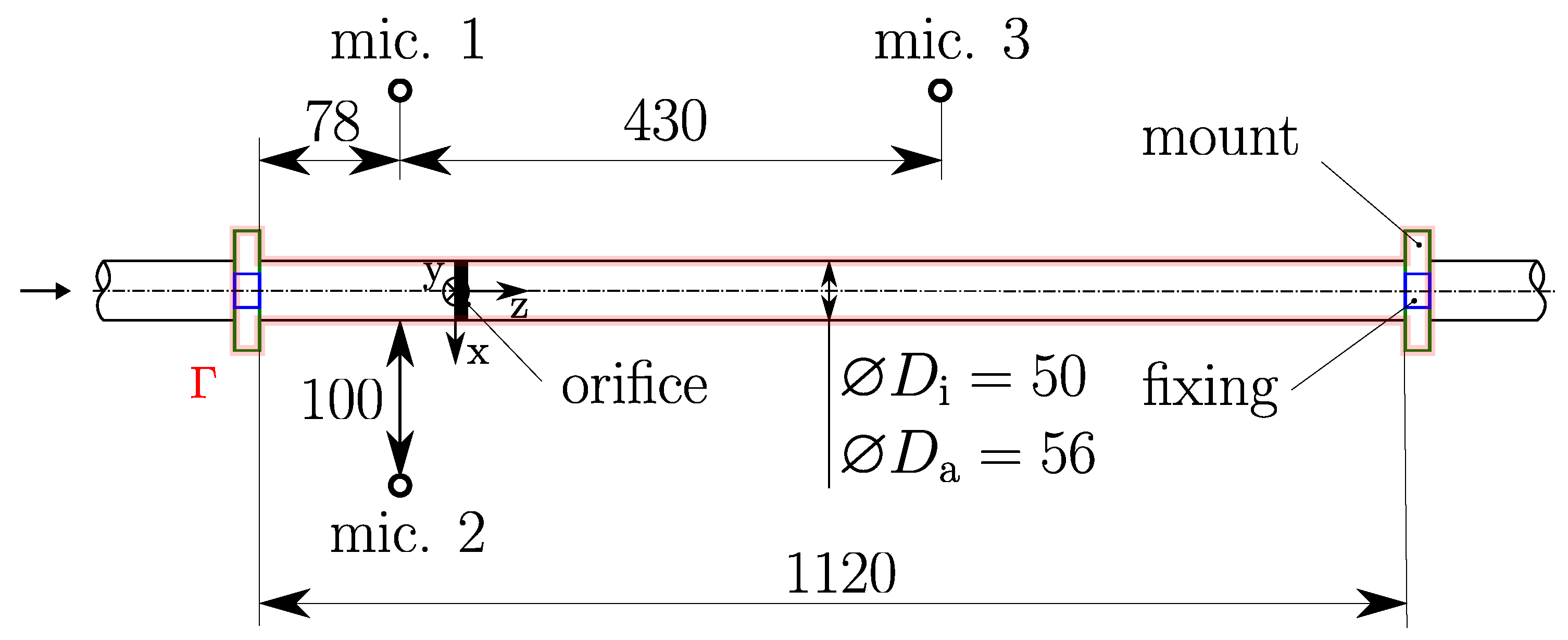
3.2. Validation Example: Pipe with Orifice

In a recent investigation, Maurerlehner et al. [21] validated a methodology employing FEM, based on the hybrid computational aeroacoustic approach, for the simulation of the acoustic field of confined flows with a modular test rig. In [28], Maurerlehner investigated the aero- and vibroacoustic sound emissions of several geometries that induce turbulence and flow instabilities, e.g., a half-moon-shaped orifice in a circular pipe. Using these results, the acoustic emissions to the free field caused by the surface vibrations of the duct will be the validation example for the proposed method. The bottom view of the geometry of this validation case is sketched in Figure 4. Therein, the duct; its mounts (i.e., the structure); and microphone positions 1, 2, and 3 are depicted. The surface $\Gamma$ used for the BEM computations is colored in red and is the outer surface of the duct wall. The interior diameter of the duct is $D_{\mathrm{i}}=50$ mm and the outer diameter is $D_{\mathrm{a}}=56$ mm.

In [28], the FE-based methodology was validated, achieving considerable agreement between the simulations and measurements of the external pressure. Building on these results, the BEM approach introduced in the present paper will be validated against the FE results and measurements. While FEM requires the volumetric computational domain that contains all points of interest to be discretized, the BEM problem is solved on the surface mesh, and an evaluation of the unknown quantity can be performed, e.g., for a limited number of arbitrary field points of interest during post-processing, hence reducing the computational complexity.

3.2.1. Measurements and FEM Model

The measurement setup for the external pressure is described in detail in Section 4.2 of [28] and will therefore only be summarized briefly in the following. The measurement data acquisition and processing are also described in detail in [21], in a case applied to internal pressure data. At the three microphone positions, mic. 1 to 3, as indicated in Figure 4, the external acoustic pressure was measured using free-field microphones (Bruel and Kjaer 4190 with preamplifier 2669 L). From the time series data, block-averaged sound pressure level (SPL) spectra were computed Equation (4.10) of [28]. This resulted in a set of measured amplitude spectra ${\left|p\right|}_m^{\mathrm{meas}}\left(f\right)$ with a mean of ${\overline{\left|p\right|}}^{\mathrm{meas}}\left(f\right)$, where $m=1,\cdots ,N^{\mathrm{meas}}$, with $N^{\mathrm{meas}}$ being the number of spectral blocks of the measurement.

The FEM setup described in [21] was used to compute the internal acoustic pressure and couple it to the structural mechanics domain (i.e., the duct wall), resulting in a surface velocity field at the outer duct surface. as described in [28]. Maurerlehner [28] also used a time-domain FEM approach for the external acoustic radiation. This resulted in a set of FEM-simulated amplitude spectra ${\left|p\right|}_n^{\mathrm{FEM}}\left(f\right)$ with their mean ${\overline{\left|p\right|}}^{\mathrm{FEM}}\left(f\right)$, where $n=1,\cdots ,N^{\mathrm{FEM}}$, with $N^{\mathrm{FEM}}$ being the number of spectral blocks in the FEM simulation.

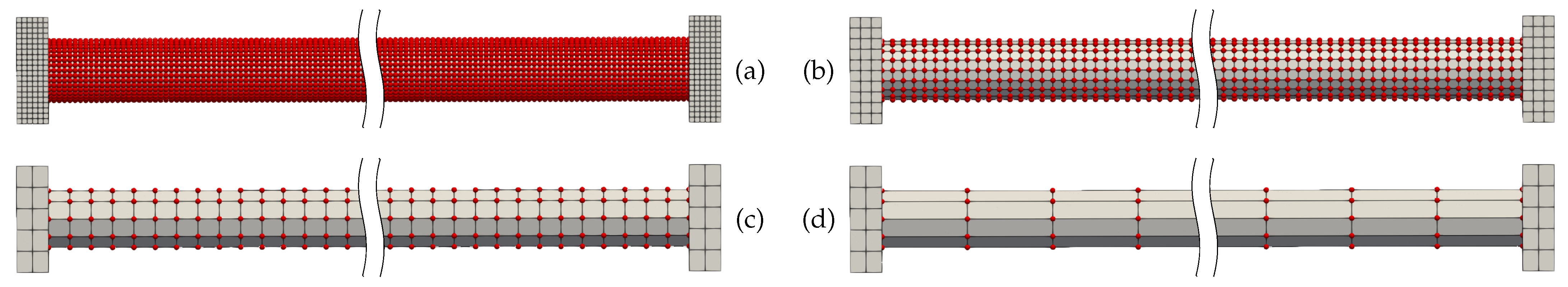
3.2.2. BEM Simulation Model

The acoustic radiation simulation was set up following the workflow described in Section 2. However, instead of taking measurements of the surface velocity, the availability of a validated FE-model of the mechanical structure allowed for extraction of the surface velocities from the (coupled) time-domain FE simulation of the pipe structure and the fluid inside [28]. Pseudo-measurement data were generated by nearest neighbor interpolation using inverse distance weighting (Shepard’s method) of the structural velocity on a grid of realistically spaced measurement points from, e.g., an LSV measurement. This approach allowed for variation of the measurement point density, which will be discussed in Section 3.2.4. For an analog comparison of the simulation results to [28], the pseudo-measurement data were split into $N^{\mathrm{BEM}}$ Hann-windowed segments of $N=2000$ samples with $50$% overlap, and point-wise Fourier transform was applied to each block. This resulted in a set of velocity spectra. The computed velocity spectra were transferred to the computational grid for the BEM simulation in the next step. The grid had equally spaced elements with an approximate element size of 5 mm, which corresponded to $6.9$ elements per wavelength at 10 $\mathrm{k}$$\mathrm{Hz}$, resulting in 10,122 degrees of freedom for the BEM formulation. The interpolation to the BEM grid was performed using the workflow presented in Section 2.1. Because of the ideal fit of the FEM surface grid to the BEM grid, however, the projection step could be skipped. The resulting spatially up-sampled data were projected in the surface normal direction according to Equation (3) and applied as a set of Neuman boundary conditions $\left[{\mathit{q}}_{\mathrm{s},1}\cdots {\mathit{q}}_{\mathrm{s},N^{\mathrm{BEM}}}\right]$ in Equation (6) to solve the discretized boundary element problem as described in Section 2.3. The acoustic pressure was evaluated at the microphone positions defined in [28] (see Figure 4). This resulted in a set of BEM-simulated amplitude spectra ${\left|p\right|}_k^{\mathrm{BEM}}\left(f\right)$ with their mean ${\overline{\left|p\right|}}^{\mathrm{BEM}}\left(f\right)$, where $k=1,\cdots ,N^{\mathrm{BEM}}$, with $N^{\mathrm{BEM}}$ being the number of spectral blocks of the BEM simulations.

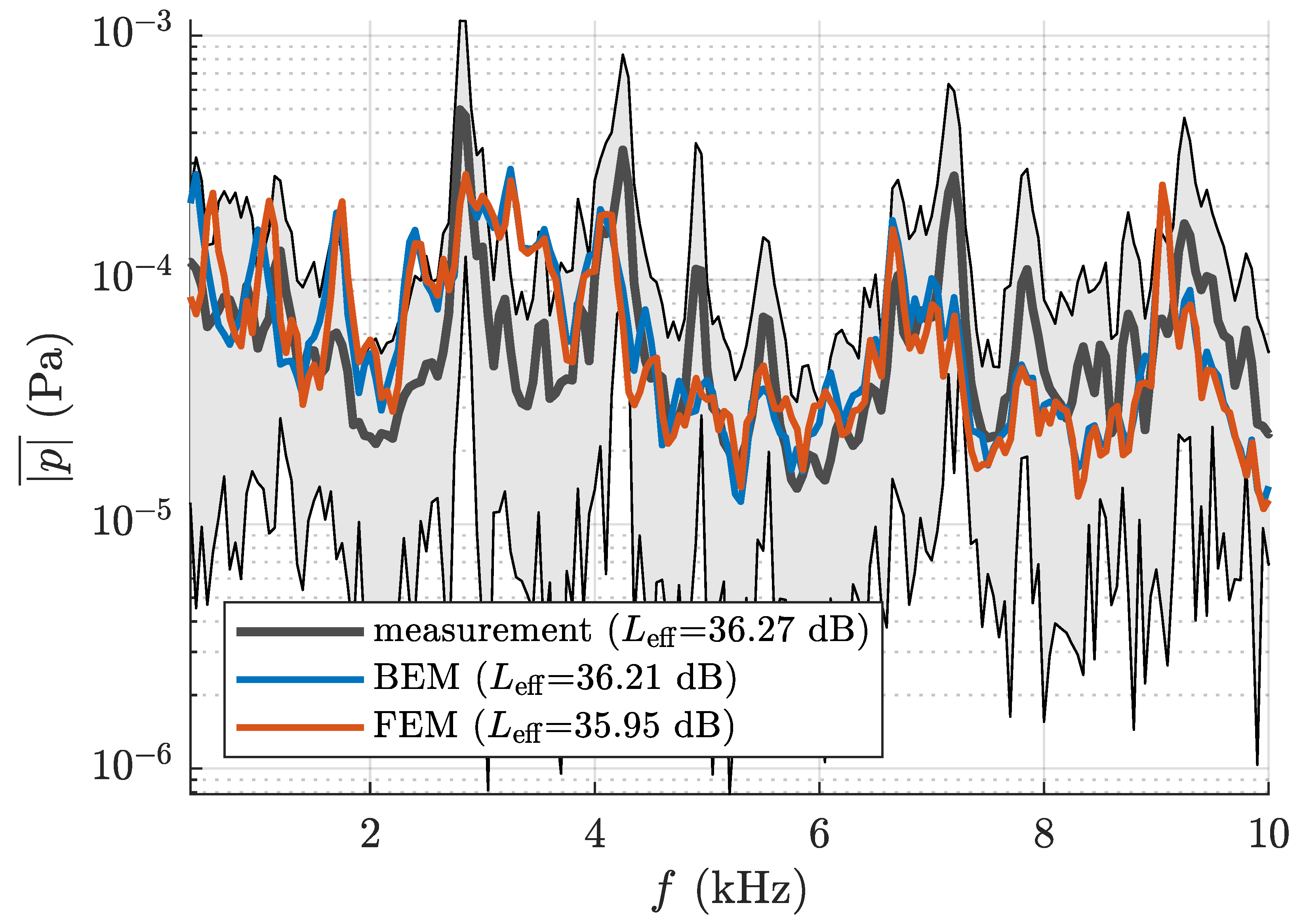
3.2.3. Comparison of Experimental and Numerical Results

A similar evaluation procedure compared the BEM method to the established FEM model in [28]. Maurerlehner [28] split the time domain pressure signals into segments of $N^{\mathrm{FEM}}=3000$ samples with 50% overlap, performed Fourier transform thereof, and computed the amplitude averaged spectra. In contrast, in this work, the time domain velocity data were split into segments of $N^{\mathrm{BEM}}=2000$ with 50% overlap. The Fourier transform of each segment resulted in multiple boundary sets for the BEM simulations. The resulting pressure spectra were amplitude averaged. Figure 5 depicts the block-averaged pressure amplitude spectrum. The legend provided an effective pressure level $L_{\mathrm{eff}}$, such that

$$L_{\mathrm{eff}}=20log\left(\frac{{∥p\left(f\right)∥}_2}{\sqrt{2}{p}_{\mathrm{ref}}}\right)\forall f\in f_{\mathrm{interest}}$$

(11)

with reference pressure $p_{\mathrm{ref}}=20$ μPa in the frequency range of interest $f_{\mathrm{interest}}=$$\left[400,10,000\right]\mathrm{Hz}$.

Table 1. Comparison of the measured and simulated effective pressure levels in the frequency range $f_{\mathrm{interest}} =\left[400,10,000\right]\mathrm{Hz}$ at the microphone positions according to Figure 4.

Microphone Position	${\mathit{L}}_{\mathbf{eff}}^{\mathbf{meas}}$	${\mathit{L}}_{\mathbf{eff}}^{\mathbf{FEM}}$	${\mathit{L}}_{\mathbf{eff}}^{\mathbf{BEM}}$	$\left|{\mathit{L}}_{\mathbf{eff}}^{\mathbf{meas}}-{\mathit{L}}_{\mathbf{eff}}^{\mathbf{BEM}}\right|$
1	$36.27$ dB	$35.95$ dB	$36.21$ dB	$0.06$ dB
2	$35.81$ dB	$35.82$ dB	$36.18$ dB	$0.37$ dB
3	$35.94$ dB	$37.87$ dB	$37.40$ dB	$1.46$ dB

shows the effective pressure levels for the measurement, FEM, and BEM simulations at the three microphone positions defined in Figure 4. The maximum deviation of the BEM solution to the FEM solution of $0.47$ dB indicated a good agreement of the presented method to the FEM simulation approach used in [28]. The simulated data agreed reasonably with the measurement data for all of the microphone positions. According to [28], deviations were caused by inaccuracies of the flow simulation data inside the pipe, the modeled mounting of the pipe, and the material damping model used, which all altered the pseudo-measurement and therefore had a similar impact on both FEM and BEM simulation approaches. Furthermore, using the acoustic free-field assumption rather than modeling the acoustic chamber introduced discrepancies between the simulation and the measurements.

Figure 5 presents a frequency-resolved evaluation of the agreement among three distinct results of the block-averaged acoustic pressure computed via the BEM and FEM results, and the empirically obtained measurement data. The FEM results were validated in this previous study [28]. Therefore, BEM is in excellent agreement with the FEM results, and only minor deviations occurred. It shows the robustness of the BEM acoustic pressure predictions. As concluded by the previous study [28], the predictions of the BEM method were validated by the measurement data at the microphone positions. The variations from numerical predictions to the multi-block averaged experimental results were well within the measurement uncertainty, indicated by the envelope of spectra of measured blocks (gray-shaded area).

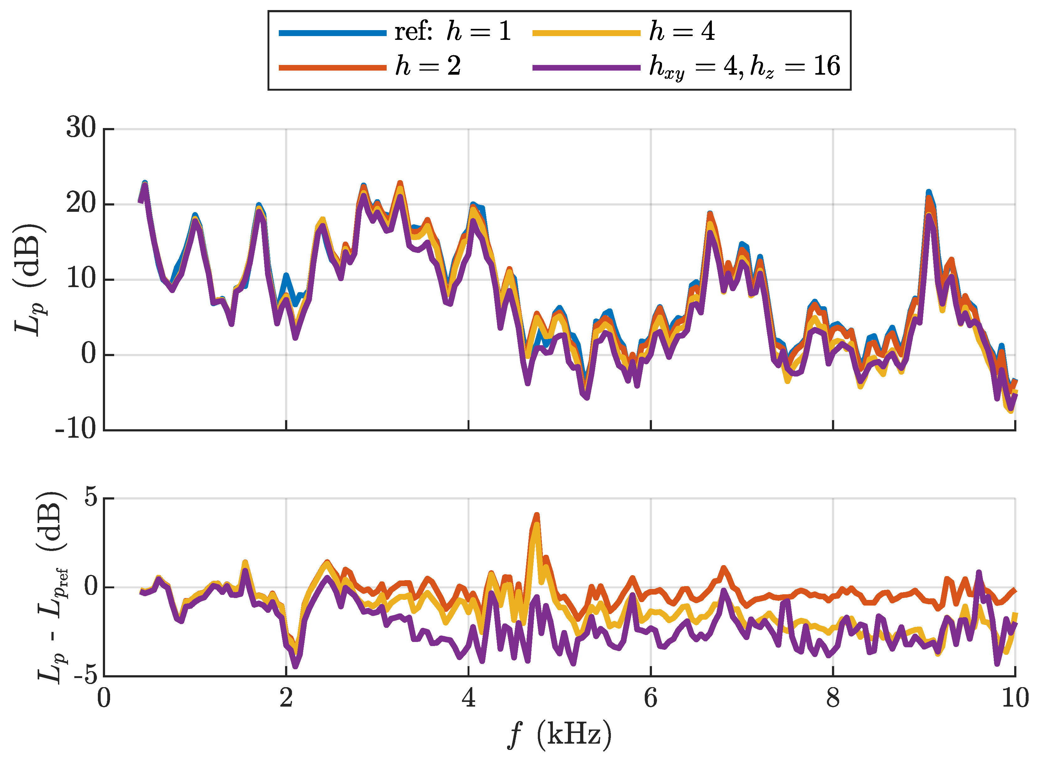
3.2.4. Variation of Measurement Point Density

The BEM solution depicted in Figure 5 was based on pseudo-measurement data that were spatially sampled with a spacing of $h_{\mathrm{ref}}=5$ mm, which matches the element size of the computational grid used for solving the sound radiation problem. In a subsequent study, the measurement point density was coarsened by multiplication of the grid distances by a factor h for all of the coordinated axes equally, or $h_x$, $h_y$, $h_z$ for each coordinate axis separately, resulting in $N_{\mathrm{LSV}}$ pseudo measurement points. The pseudo measurement grids considered in the study are depicted in Figure 6.

Figure 7 depicts the acoustic pressure level $L_p=20log\left(p/p_{\mathrm{ref}}\right)$, and its deviation from the reference BEM simulation results. The comparison was two-fold. Firstly, the acoustic pressure levels were compared as a function of frequency. From this perspective, deviations to the reference signals were small, and good agreement was also achieved for very poorly resolved measured surface velocities. Secondly, to evaluate the differences in more detail, the relative difference to the reference was plotted as a function of frequency. This shows a very clear trend: the deviations between the h-dependent simulated acoustic pressure levels and the reference simulation results ($h=1$) systematically increased with the frequency. At certain frequencies, 2100 $\mathrm{Hz}$ and 4750 $\mathrm{Hz}$, the deviations were large and increased until a range of 5 dB. At these frequencies, structural anti-resonances mitigated the large-scale motion, and the measured data did not resolve the remaining motion. The increasing deviations with frequency were expected and could be attributed to the reduced resolution per wavelength of the interpolated surface velocity data. The second effect, which was visible, was that with decreasing resolution (increasing h) of the measured surface velocities, the deviations became larger, and in general, the radiated sound pressure levels were underestimated. Again, this can be explained by the reduced resolution of the structural motion and due to the linear interpolation scheme, which underestimated the movement of convex curved surfaces. In summary, Figure 7 demonstrates how the acoustic pressure level deviations in a simulation changed with both the frequency and spatial resolution of the structural motion. As the structural wavelengths were large compared with the acoustic wavelength, the surface velocity required less spatial resolution in the presented benchmark problem.

4. Application: Prosthesis Frame

The previously verified and validated simulation setup consisting of the interpolation algorithm and the acoustic propagation simulation using BEM was applied to an industrial problem. Thereby, the acoustic radiation of a clinically applied knee prosthesis frame was investigated by means of measurements and simulations. The prosthesis frame (device unter test—DUT) had dimensions of $\left(270\times 80\times 100 \mathrm{mm}\right)$ and was made of carbon-fiber reinforced plastic with titanium inserts. The complex material behavior made it difficult to accurately predict the structural dynamics using FE simulation and experimental acquisition of the surface vibration was preferred.

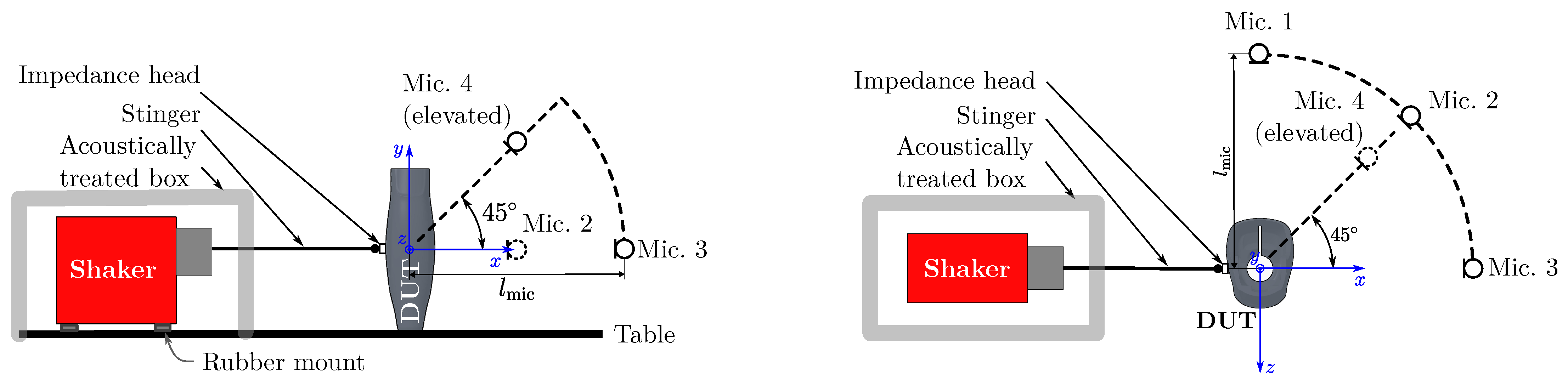
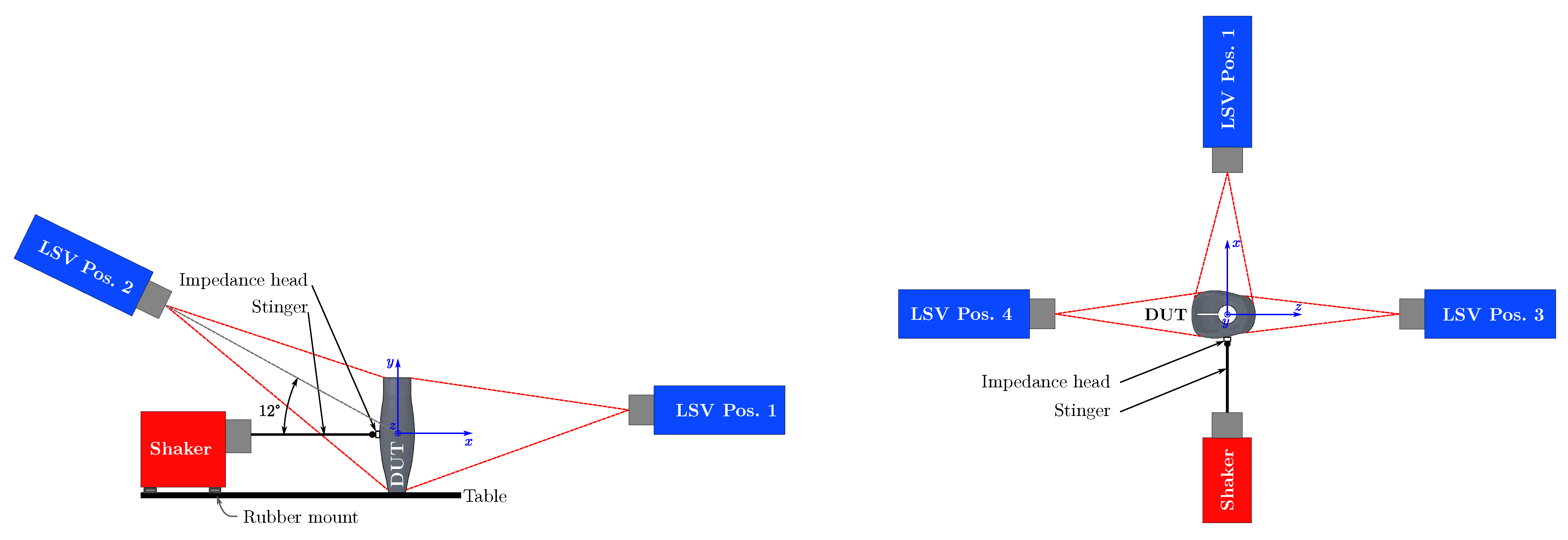
4.1. Measurement Setup

The measurement environment for both the microphone and LSV measurements was an acoustically treated chamber of type Studiobox Premium with a size of $3.0\times 2.02\times 2.3$ m. The prosthesis frame (device under test—DUT) was positioned centrally in the room on a table together with the shaker (DynaLabs DYN-PM-100), which was connected to the DUT by a stinger. The shaker was mounted on rubber elements to decouple it mechanically from the table. Furthermore, an acoustically treated box was placed over the shaker to minimize the influence of the sound emissions of the shaker on the measurement setup. To measure the input force, an impedance head (DJB AF/100/10) was applied at the stinger–DUT connection, allowing for measurements of the input force $F\left(t\right)$ on the DUT. The excitation signal was a pseudo-random noise that was generated by the control unit of the LSV for a frequency range from $2\mathrm{Hz}$ to $6.4$ kHz with a desired frequency resolution of $2\mathrm{Hz}$ (corresponding to 3200 spectral lines). Together with a sampling frequency of $16$ kHz, this resulted in a measurement time of $0.5$ s. Using this setup, the microphone measurements obtaining the acoustic pressure and the surface velocity measurements with the LSV were conducted as described in the following.

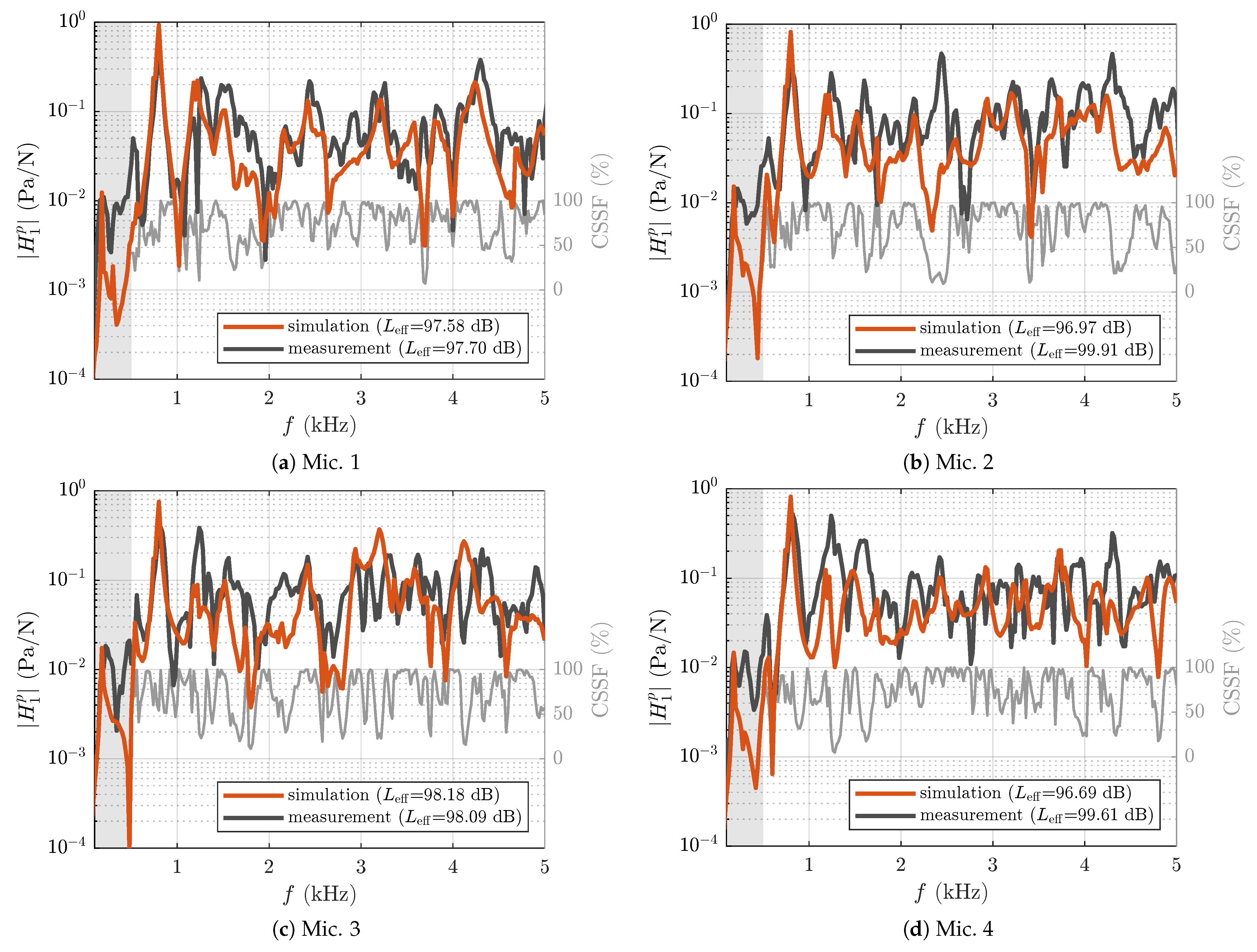
4.1.1. Acoustic Pressure Measurements

The setup of the acoustic measurements using four microphone positions is depicted schematically in Figure 8 in a side and top view. Four microphones (Bruel and Kjaer 4189 free-field microphones ) were placed at a distance of $l_{\mathrm{mic}}=0.7$ m around the DUT, obtaining the acoustic pressure. Microphones 1, 2, and 3 were located in the $x/z$-plane at $y=0$. Microphone 4 was at a $45{}^{\circ }$ elevation. The microphone signals in time domain were denoted as $p^{\mathrm{mic}1}\left(t\right)$, $p^{\mathrm{mic}2}\left(t\right)$, $p^{\mathrm{mic}3}\left(t\right)$, and $p^{\mathrm{mic}4}\left(t\right)$ for microphones 1 to 4, respectively.

The microphones were connected to a data acquisition unit (HEAD acoustics SQuadriga III) handling the analog/digital conversion. The time series measurements of the acoustic pressure and the input force with a sampling frequency of $f_S=48$ kHz were buffered into blocks with a length of $N_{\mathrm{samp}}=2400$ samples and 50% overlap, corresponding to a target frequency resolution of $\Delta f=20\mathrm{Hz}$. A Hann window function was applied on each block. For each block, the $N_{\mathrm{samp}}$-point Discrete Fourier Transform (DFT) was performed as implemented in MATLAB’s stft()-command [29], which resulted in pressure spectra ${\tilde{p}}_i^{\mathrm{mic}1}\left(f\right)$, ${\tilde{p}}_i^{\mathrm{mic}2}\left(f\right)$, ${\tilde{p}}_i^{\mathrm{mic}3}\left(f\right)$, and ${\tilde{p}}_i^{\mathrm{mic}4}\left(f\right)$ for microphones 1 to 4, respectively, as well as ${\tilde{F}}_i\left(f\right)$ for the input force spectrum. Thereby, $i=1,\cdots ,N_{\mathrm{blocks}}$, where $N_{\mathrm{blocks}}$ is the number of blocks, which is equal to the number of spectra after DFT. The transfer function $H_1^u\left(f\right)$ from the input force F to a quantity of interest u was computed using

$$H_1^u\left(f\right)=\frac{G_{\mathrm{uF}}}{G_{\mathrm{FF}}},$$

(12)

where $G_{\mathrm{uF}}$ is the cross power spectral density between the quantity of interest u and the input force F, and $G_{\mathrm{FF}}$ is the auto power density spectrum of the input force F. $G_{\mathrm{uF}}$ and $G_{\mathrm{FF}}$ are computed from

$$G_{\mathrm{uF}}=\frac{1}{N_{\mathrm{blocks}}}\sum _{i=1}^{N_{\mathrm{blocks}}}{u}_i\left(f\right){\tilde{F}}_i^{*}\left(f\right),G_{\mathrm{FF}}=\frac{1}{N_{\mathrm{blocks}}}\sum _{i=1}^{N_{\mathrm{blocks}}}{\tilde{F}}_i\left(f\right){\tilde{F}}_i^{*}\left(f\right),$$

(13)

where superscript ${}^{*}$ denotes the complex conjugate. The quantity of interest $u_i\left(f\right)$ is one of the pressure spectra ${\tilde{p}}_i^{\mathrm{mic}1}\left(f\right)$, ${\tilde{p}}_i^{\mathrm{mic}2}\left(f\right)$, ${\tilde{p}}_i^{\mathrm{mic}3}\left(f\right)$, or ${\tilde{p}}_i^{\mathrm{mic}4}\left(f\right)$, such that $H_1^p\left(f\right)$ is the desired vibroacoustic transfer function. This resulted in one transfer function for each microphone position and, thus, four transfer functions in total.

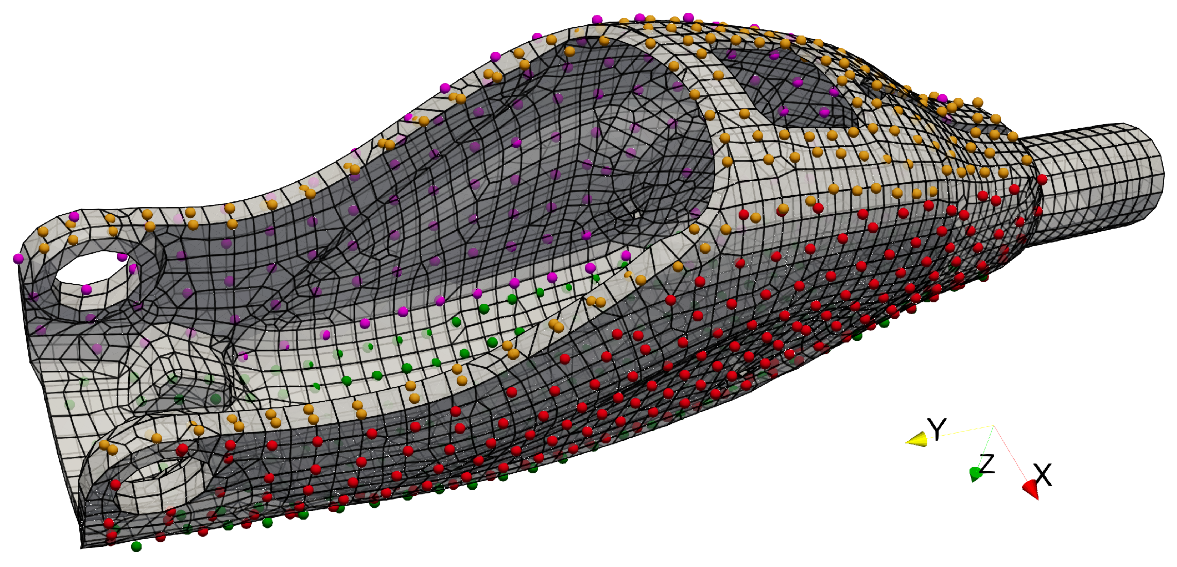
4.1.2. Surface Velocity Measurements Using LSV

The surface velocity of the DUT was measured using an LSV (Polytec PSV-500 Xtra), as described in Section 2.1. The LSV was positioned in four positions, as depicted in Figure 9, such that the whole DUT surface could be measured. This resulted in an overall number of measurement points $N_{\mathrm{LSV}}=688$. Figure 10 shows the distribution of scanning points for each measurement patch. The four patches of the measurement data were combined during the data transfer process described in Section 4.2.

From the measured surface velocity and the input forces, a transfer function from input force F to surface velocity v was computed with Equations (12) and (13). Thereby, the quantity of interest u is the velocity spectrum. This form of the $H_1^v\left(f\right)$ transfer function is the so-called mobility (p. 52, [30]). The measurement data post-processing was performed using the software Polytec PSV Software, which directly computed the mobility transfer functions.

4.2. BEM Simulation Model

The simulation model was set up according to Section 2.3. Therefore, the surface of a CAD representation of DUT, ${\Gamma }_{\mathrm{s}}$, was discretized with linear quadrilateral and triangular elements with an approximate edge length of 6 $\mathrm{m}$$\mathrm{m}$, resolving the maximum frequency of interest at 5 $\mathrm{k}$$\mathrm{Hz}$ with approximately 11.4 elements per wavelength. This resulted in 7158 degrees of freedom. The computational grid is depicted in Figure 10. The mobility transfer function $H_1^v$ was transferred to ${\Gamma }_{\mathrm{s}}$ using the presented workflow in Section 2.1 for each measurement patch individually, and subsequently summed up. It should be noted that the summation of the velocity components was feasible, as the measurement directions of the measurement patches that shared overlapping regions were approximately orthogonal, and thus the resulting velocity vector did not overestimate the true velocity in any direction. Furthermore, inside non-overlapping regions, the measurement direction was chosen to match the normal direction of each surface patch as well as possible. One-dimensional LSV measurement of oblique-angled motion led to a geometrically induced systematic error [31]. Concerning these systematic errors, deviations in measurement direction from the surface normal direction led to an underestimation of the radiated sound. For high wave numbers, a phase error could also be significant. In general, a comparison of the obtained surface velocity data to single-point measurements or a 3D-LSV measurement might be required to approve the usage of 1D LSV data. Areas of the DUT that were inaccessible for measurement were set to zero. Thin structures were assumed as thin plates, based on the Kirchhoff–Love plate theory, and, therefore, only flexural plate waves were considered. Consequently, the inner wall surfaces were projected onto the measurement patches of the outer surfaces. All of the aforementioned simplifying assumptions should result in underestimating the radiated sound power, as parts of the DUT’s oscillation were neglected. Potentially, neglecting destructive local acoustic effects could also lead to overestimating the radiated sound; however, this would be unlikely at low frequencies. The mobility data on ${\Gamma }_{\mathrm{s}}$ were then interpolated onto the element centers and projected in the normal direction of the respective element. Finally, the Neumann boundary condition was computed according to Equation (8), modeling the acoustic radiation due to a unit force excitation yielding the vibroacoustic transfer function $H_1^p$.

4.3. Comparison of Measurement and Simulation

The vibroacoustic $H_1^p$ transfer functions computed from the force measurement and microphone measurements or LSV measurement in combination with BEM simulation, respectively, are depicted in Figure 11. For all four of the evaluated positions, good agreement between the two workflows was achieved. Resonance peaks in the transfer function due to resonance of the structural-mechanical system, the acoustic system, or coupled resonance were captured equally well, especially at medium frequencies. In the low-frequency range below 500 $\mathrm{Hz}$, the microphone measurement overestimated the transfer function compared with the simulation approach. While the used anechoic room was found to guarantee sufficient insulation from the environment above 100 $\mathrm{Hz}$, acoustic free-field conditions were violated with a significant increase in reverberation time below 250 $\mathrm{Hz}$, based on the manufacturer’s information. Furthermore, reference measurements of the sound field with a removed stinger connection from the shaker to the DUT revealed significant inefficiency in the decoupling of the shaker with SPL being approximately 10 dB higher below 500 $\mathrm{Hz}$ to the higher frequency range. Especially at 300 $\mathrm{Hz}$ and 480 $\mathrm{Hz}$, resonance peaks could be observed. This behavior was most definitely caused by the inefficient decoupling of the shaker from the measurement environment both mechanically via induced vibrations to the table and acoustically due to insufficient acoustic insulation of the shaker.

A quantitative measure of similarity between two frequency response functions was provided by the Cross Signature Scale Factor (CSSF) [32], which is a frequency-dependent comparison yielding a value in the interval $[0,1]$. From the measured transfer function $H_{1,\mathrm{meas}}^p$ and the simulated transfer function $H_{1,\mathrm{sim}}^p$, CSSF was computed with Equation (2) of [32], such that

$$CSSF\left(f\right)=\frac{2\left|{\left(H_{1,\mathrm{meas}}^p\left(f\right)\right)}^{*}·H_{1,\mathrm{sim}}^p\left(f\right)\right|}{{\left(H_{1,\mathrm{meas}}^p\left(f\right)\right)}^{*}·H_{1,\mathrm{meas}}^p\left(f\right)+{\left(H_{1,\mathrm{sim}}^p\left(f\right)\right)}^{*}·H_{1,\mathrm{sim}}^p\left(f\right)},$$

(14)

where superscript ${}^{*}$ denotes the complex conjugate. A CSSF value close to 100% indicates excellent agreement of the transfer functions. In Figure 11, CSSF is plotted together with the measured and simulated transfer functions. Therefrom, it is clear that the simulation was able to predict the transfer function with a high degree of conformity over a large frequency range.

Table 2. Effective pressure level for a unit force excitation in the frequency range $f_{\mathrm{interes}} =\left[500,5000\right]\mathrm{Hz}$ at the microphone positions according to Figure 8.

Microphone Position	${\mathit{L}}_{\mathbf{eff}}^{\mathbf{meas}}$	${\mathit{L}}_{\mathbf{eff}}^{\mathbf{BEM}}$	$\left|{\mathit{L}}_{\mathbf{eff}}^{\mathbf{meas}}-{\mathit{L}}_{\mathbf{eff}}^{\mathbf{BEM}}\right|$
1	$97.70$ dB	$97.58$ dB	$0.12$ dB
2	$99.91$ dB	$96.97$ dB	$2.94$ dB
3	$98.09$ dB	$98.18$ dB	$0.09$ dB
4	$99.61$ dB	$96.69$ dB	$2.92$ dB

lists the effective pressure level for a unit force excitation, as defined in (11) in the frequency range $f_{\mathrm{interes}}=\left[500,5000\right]\mathrm{Hz}$. The maximum deviation of the simulation approach to the acoustic measurement of $2.94$ dB indicates a good prediction of the average vibroacoustic transfer path in the medium- to high-frequency range above 500 $\mathrm{Hz}$. In general, a slight underestimation of the measured amplitude spectra could be observed in this frequency range. This behavior could be explained by the simplifications discussed in Section 4.2. Furthermore, the oblique laser direction, which does not coincide with the normal velocity at every measurement point, could contribute to the deviations. Larger deviations at certain microphone positions and frequencies, e.g., at the position of Mic. 2 in the interval $\left[2,3\right]\mathrm{k}\mathrm{Hz}$, could be due to the imperfect free-field in the experimental setup.

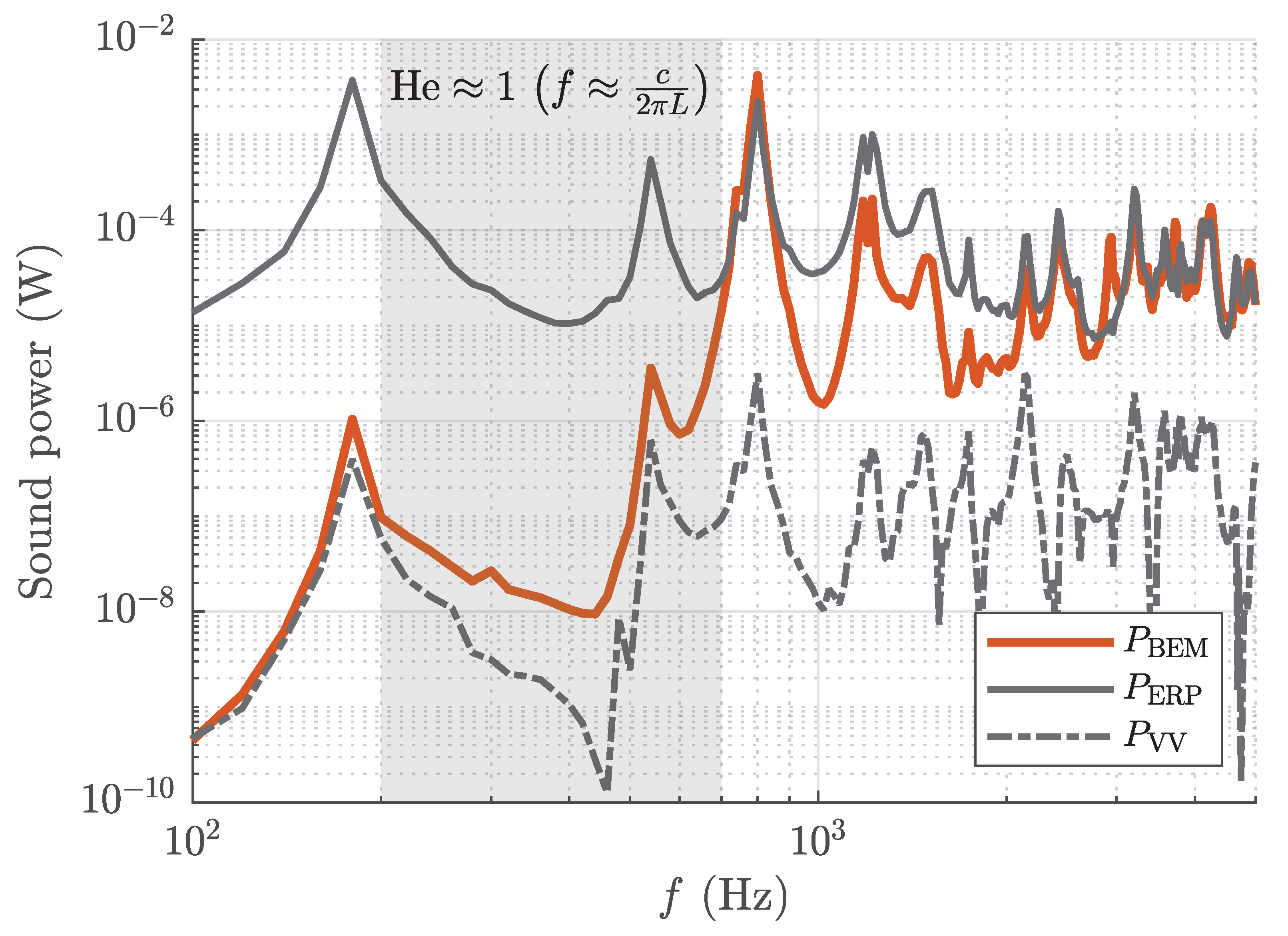
4.4. Radiated Sound Power

One of the most important quantities to assess the sound emissions of a machine or product is the radiated sound power $P={\oint }_{\Gamma }\mathit{I}·\mathit{n}\mathrm{d}\Gamma$, with the acoustic intensity $\mathit{I}=\frac{1}{2}\Re \left\{p{\mathit{v}}^{*}\right\}$, and the conjugate complex indicated by superscript ${}^{*}$. Having solved the BEM problem as defined in Section 4.2, and achieved acceptable agreement with validation measurements, as discussed in Section 4.3, the sound power can be calculated by

$$P_{\mathrm{BEM}}=\frac{1}{2}{\int }_{{\Gamma }_{\mathrm{s}}}\Re \left\{\frac{p_{\mathrm{s}}{q}_{\mathrm{s}}^{*}}{-\mathrm{j}\omega \rho }\right\}\mathrm{d}\Gamma ,$$

(15)

using Equation (8). Figure 12 shows the predicted sound power in comparison with the common low-cost approximations based on the equivalent radiated power (ERP) $P_{\mathrm{ERP}}$ or based on the volume velocity $P_{\mathrm{VV}}$, as defined in Equations (10) and (19) of [22], respectively. The two low-cost approximations can be understood as qualitative upper and lower bounds for vibroacoustically emitted sound power. ERP uses the far-field approximation, resulting in a constant radiation efficiency $\sigma =1$ for all surface areas and neglecting local acoustic effects. Therefore, dipole effects (antiphase vibration of the sources) were not captured, and the radiated sound power was overestimated in the low-frequency range. Towards higher frequencies, these effects were less significant, and thus the deviation decreased. In contrast, the sound power approximation based on the volume velocity assumed an acoustically compact source, which was only viable in the very low-frequency range. Both estimates could be evaluated explicitly as simple summations without the need to assemble a system matrix and thus could be computed in the order of seconds on any state-of-the-art notebook. In contrast, BEM, as presented in Section 2.2, required an assembly of system matrices, and resulted in an algebraic system of equations that needed to be solved. The presented simulation of the prosthesis’ frame required approx. 14 $\mathrm{h}$ on a single CPU-core of the used system, but it scaled well on a multi-core CPU, reducing the actual computation time to approx. 14 $\min$. The computations were performed on a single compute node of the Vienna Scientific Cluster (VSC) equipped with an AMD EPYC 7713 (64 core) CPU, and 512 GB RAM. Consequently, an estimate of where to use the presented BEM approach was viewed as useful to the authors. The frequency range in which the radiated sound power based on BEM simulation deviated from both approximations is given by the Helmholtz number $\mathrm{He}=\frac{L}{\lambda }=kL\approx 1$ with length scale L. Consequently, if the frequency range of interest intersects with

$$f\approx \frac{c}{2\pi L},$$

(16)

the BEM approach has to be used to produce accurate predictions. Choosing L as the main dimensions of DUT results in $\mathrm{He}\approx 1$ in the frequency range $f\approx \left[200,700\right]\mathrm{Hz}$, which agrees with the results shown in Figure 12.

5. Discussion

This paper presents a simulation approach based on BEM, which utilizes interpolated surface velocities as the boundary conditions. The interpolation algorithm for the surface velocities is based on evaluating the finite element basis functions at the target mesh. A verification of the BEM solver was achieved in a previous study. For validating the simulation approach, surface velocities simulated by FEM were taken as inputs with varying mesh sizes. The acoustic propagation results of the validation simulation computed with BEM were in very good agreement with measurements and the comparison simulation with FEM, as shown in Table 1. After applying the verified and validated simulation approach to compute the acoustic radiations of a clinically applied knee prosthesis frame, very good agreements were found between the simulated and measured effective acoustic pressure levels, as shown in Table 2.

Acoustic propagation simulations using BEM implies ideal free-field radiation conditions for the whole frequency range. For low frequencies, this can not be easily achieved in real-world measurement environments, such as anechoic chambers. Therefore, the presented method allows for the prediction of free-field acoustic emissions based solely on LSV measurements, which can also be performed under non-ideal acoustic conditions, i.e., a general room that is not anechoic, provided that no acoustic feedback occurs. In addition, based on the sound emission simulation results, further acoustic quantities, such as the free-field radiated acoustic power, can be evaluated. This can be especially useful, if the frequency of interest is close to $\mathrm{He}\approx 1$, where other low-cost approximation methods fail to provide accurate predictions for the radiated acoustic power.

Finally, the fact that the validation example and its application to a real-world problem exhibit very good agreements between (i) the BEM simulation results, (ii) the FEM results, and (iii) acoustic pressure measurements suggests that the presented approach may generalize well to other problems with a similar geometric complexity.

References

- Christensen, R. Acoustic Modeling of Hearing Aid Components. Ph.D. Thesis, Syddansk Universitet, Odense, Denmark, 2010. [Google Scholar]
- Candy, J. Accurate calculation of radiation and diffraction from loudspeaker enclosures at low frequency. J. Audio Eng. Soc. 2013, 61, 356–365. [Google Scholar]
- Nuraini, A.; Mohd Ihsan, A.; Nor, M.; Jamaluddin, N. Vibro-acoustic analysis of free piston engine structure using finite element and boundary element methods. J. Mech. Sci. Technol. 2012, 26, 2405–2411. [Google Scholar] [CrossRef]
- Panda, K.C. Dealing with noise and vibration in automotive industry. Procedia Eng. 2016, 144, 1167–1174. [Google Scholar] [CrossRef]
- Oberst, S.; Lai, J.; Marburg, S. Guidelines for numerical vibration and acoustic analysis of disc brake squeal using simple models of brake systems. J. Sound Vib. 2013, 332, 2284–2299. [Google Scholar] [CrossRef]
- Bates, T.P.; Bacon, I.C.; Blotter, J.D.; Sommerfeldt, S.D. Vibration-based sound power measurements of arbitrarily curved panels. J. Acoust. Soc. Am. 2022, 151, 1171–1179. [Google Scholar] [CrossRef] [PubMed]
- Yeh, F.; Chang, X.; Sung, Y. Numerical and Experimental Study on Vibration and Noise of Embedded Rail System. J. Appl. Math. Phys. 2017, 5, 1629. [Google Scholar] [CrossRef]
- Vlahopoulos, N.; Vallance, C.; Stark, R.D., III. Numerical approach for computing noise-induced vibration from launch environments. J. Spacecr. Rocket. 1998, 35, 355–360. [Google Scholar] [CrossRef]
- Rossignol, K.S.; Lummer, M.; Delfs, J. Validation of DLR’s sound shielding prediction tool using a novel sound source. In Proceedings of the 15th AIAA/CEAS Aeroacoustics Conference (30th AIAA Aeroacoustics Conference), Miami, FL, USA, 11–13 May 2009; p. 3329. [Google Scholar] [CrossRef]
- Lummer, M.; Akkermans, R.A.; Richter, C.; Pröber, C.; Delfs, J. Validation of a model for open rotor noise predictions and calculation of shielding effects using a fast BEM. In Proceedings of the 19th AIAA/CEAS Aeroacoustics Conference, Berlin, Germany, 27–29 May 2013; p. 2096. [Google Scholar] [CrossRef]
- Kumar, S.; Forster, H.M.; Bailey, P.; Griffiths, T.D. Mapping unpleasantness of sounds to their auditory representation. J. Acoust. Soc. Am. 2008, 124, 3810–3817. [Google Scholar] [CrossRef]
- Preuss, S.; Gurbuz, C.; Jelich, C.; Baydoun, S.K.; Marburg, S. Recent advances in acoustic boundary element methods. J. Theor. Comput. Acoust. 2022, 30, 2240002. [Google Scholar] [CrossRef]
- Fritze, D.; Marburg, S.; Hardtke, H.J. FEM–BEM-coupling and structural–acoustic sensitivity analysis for shell geometries. Comput. Struct. 2005, 83, 143–154. [Google Scholar] [CrossRef]
- Kirkup, S. The boundary element method in acoustics: A survey. Appl. Sci. 2019, 9, 1642. [Google Scholar] [CrossRef]
- Li, Y.; Meyer, J.; Lokki, T.; Cuenca, J.; Atak, O.; Desmet, W. Benchmarking of finite-difference time-domain method and fast multipole boundary element method for room acoustics. Appl. Acoust. 2022, 191, 108662. [Google Scholar] [CrossRef]
- Chen, L.; Lian, H.; Natarajan, S.; Zhao, W.; Chen, X.; Bordas, S. Multi-frequency acoustic topology optimization of sound-absorption materials with isogeometric boundary element methods accelerated by frequency-decoupling and model order reduction techniques. Comput. Methods Appl. Mech. Eng. 2022, 395, 114997. [Google Scholar] [CrossRef]
- Deckers, E.; Atak, O.; Coox, L.; D’Amico, R.; Devriendt, H.; Jonckheere, S.; Koo, K.; Pluymers, B.; Vandepitte, D.; Desmet, W. The wave based method: An overview of 15 years of research. Wave Motion 2014, 51, 550–565. [Google Scholar] [CrossRef]
- Schoder, S.; Roppert, K. openCFS-Data: Data Pre-Post-Processing Tool for openCFS–Aeroacoustics Source Filters. arXiv 2023, arXiv:2302.03637. [Google Scholar] [CrossRef]
- Marburg, S. Boundary Element Method for Time-Harmonic Acoustic Problems. In Computational Acoustics; Kaltenbacher, M., Ed.; Springer International Publishing: Cham, Switzerland, 2018; pp. 69–158. [Google Scholar] [CrossRef]
- Fiala, P.; Rucz, P. NiHu: An open source C++ BEM library. Adv. Eng. Softw. 2014, 75, 101–112. [Google Scholar] [CrossRef]
- Maurerlehner, P.; Schoder, S.; Tieber, J.; Freidhager, C.; Steiner, H.; Brenn, G.; Schäfer, K.H.; Ennemoser, A.; Kaltenbacher, M. Aeroacoustic formulations for confined flows based on incompressible flow data. Acta Acust. 2022, 6, 45. [Google Scholar] [CrossRef]
- Fritze, D.; Marburg, S.; Hardtke, H.J. Estimation of radiated sound power: A case study on common approximation methods. Acta Acust. United Acust. 2009, 95, 833–842. [Google Scholar] [CrossRef]
- Rothberg, S.; Allen, M.; Castellini, P.; Di Maio, D.; Dirckx, J.; Ewins, D.; Halkon, B.; Muyshondt, P.; Paone, N.; Ryan, T.; et al. An international review of laser Doppler vibrometry: Making light work of vibration measurement. Opt. Lasers Eng. 2017, 99, 11–22. [Google Scholar] [CrossRef]
- Burton, A.J.; Miller, G.F. The application of integral equation methods to the numerical solution of some exterior boundary-value problems. Proc. R. Soc. Lond. 1971, 323, 201–210. [Google Scholar] [CrossRef]
- Marburg, S. The Burton and Miller Method: Unlocking Another Mystery of Its Coupling Parameter. J. Comput. Acoust. 2016, 24, 1550016. [Google Scholar] [CrossRef]
- Fiala, P.; Rucz, P. NiHu: A multi-purpose open source fast multipole solver. In Proceedings of the DAGA 2019. German Acoustical Society (DEGA), Rostock, Germany, 18–21 March 2019; pp. 1262–1265. [Google Scholar]
- Schenck, H.A. Improved Integral Formulation for Acoustic Radiation Problems. J. Acoust. Soc. Am. 1968, 44, 41–58. [Google Scholar] [CrossRef]
- Maurerlehner, P. Aero- and Vibroacoustics of Confined Flows. Ph.D. Thesis, TU Graz, Graz, Austria, 2023. [Google Scholar]
- Mathworks. Matlab documentation: (). 2023. Available online: https://de.mathworks.com/help/signal/ref/stft.html (accessed on 11 October 2023).
- Avitabile, P. Modal Testing: A Practitioner’s Guide; John Wiley & Sons Ltd: Chichester, UK, 2017. [Google Scholar] [CrossRef]
- Neumann, M.N.; Hennings, B.; Lammering, R. Identification and Avoidance of Systematic Measurement Errors in Lamb Wave Observation With One-Dimensional Scanning Laser Vibrometry. Strain 2013, 49, 95–101. [Google Scholar] [CrossRef]
- Dascotte, E.; Strobbe, J. Updating finite element models using FRF correlation functions. In Proceedings of the 17th International Modal Analysis Conference, Kissimmee, FL, USA, 8–11 February 1999; pp. 1169–1174. [Google Scholar]