
IIR Cascaded-Resonator-Based Complex Filter Banks


Abstract
:
1. Introduction
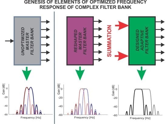
2. Design Method
2.1. Problem Statement
2.2. Design (Optimization) Approach 1—Linear Least-Squares Minimization
2.3. Design (Optimization) Approach 2—Minimax Optimization
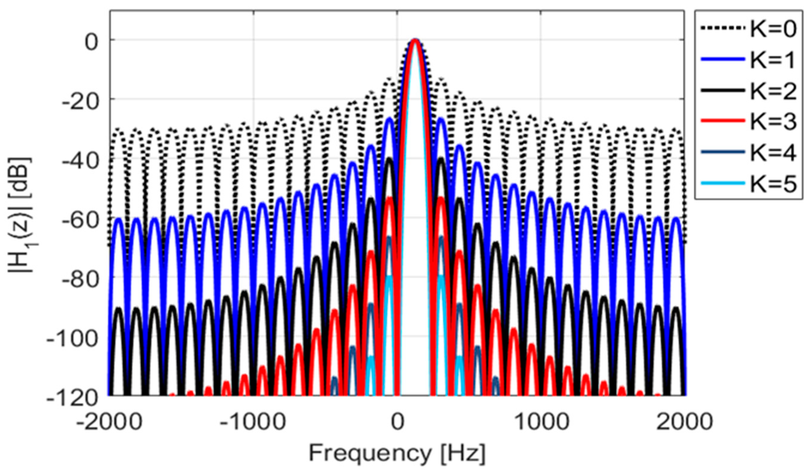
2.4. Sidelobe Constraints (Frequency Response Constraints in Stop Bands)
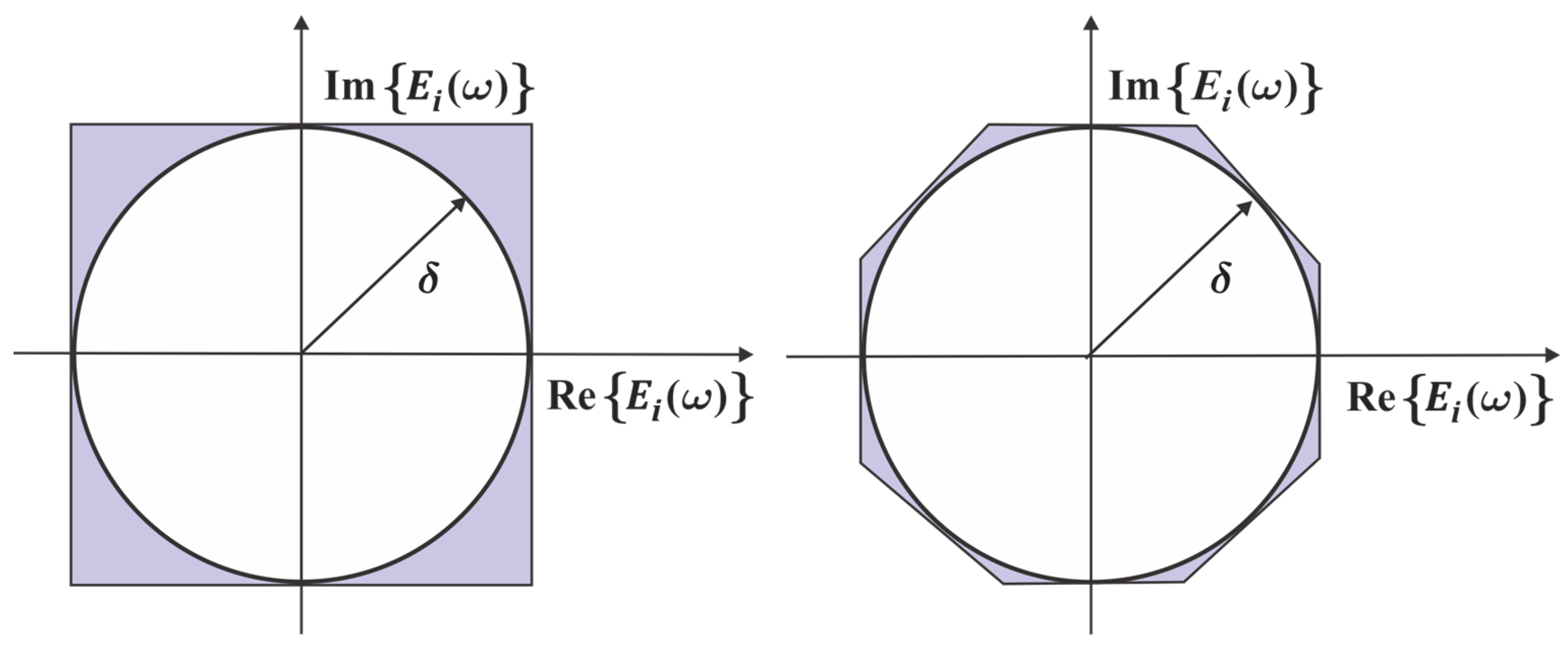
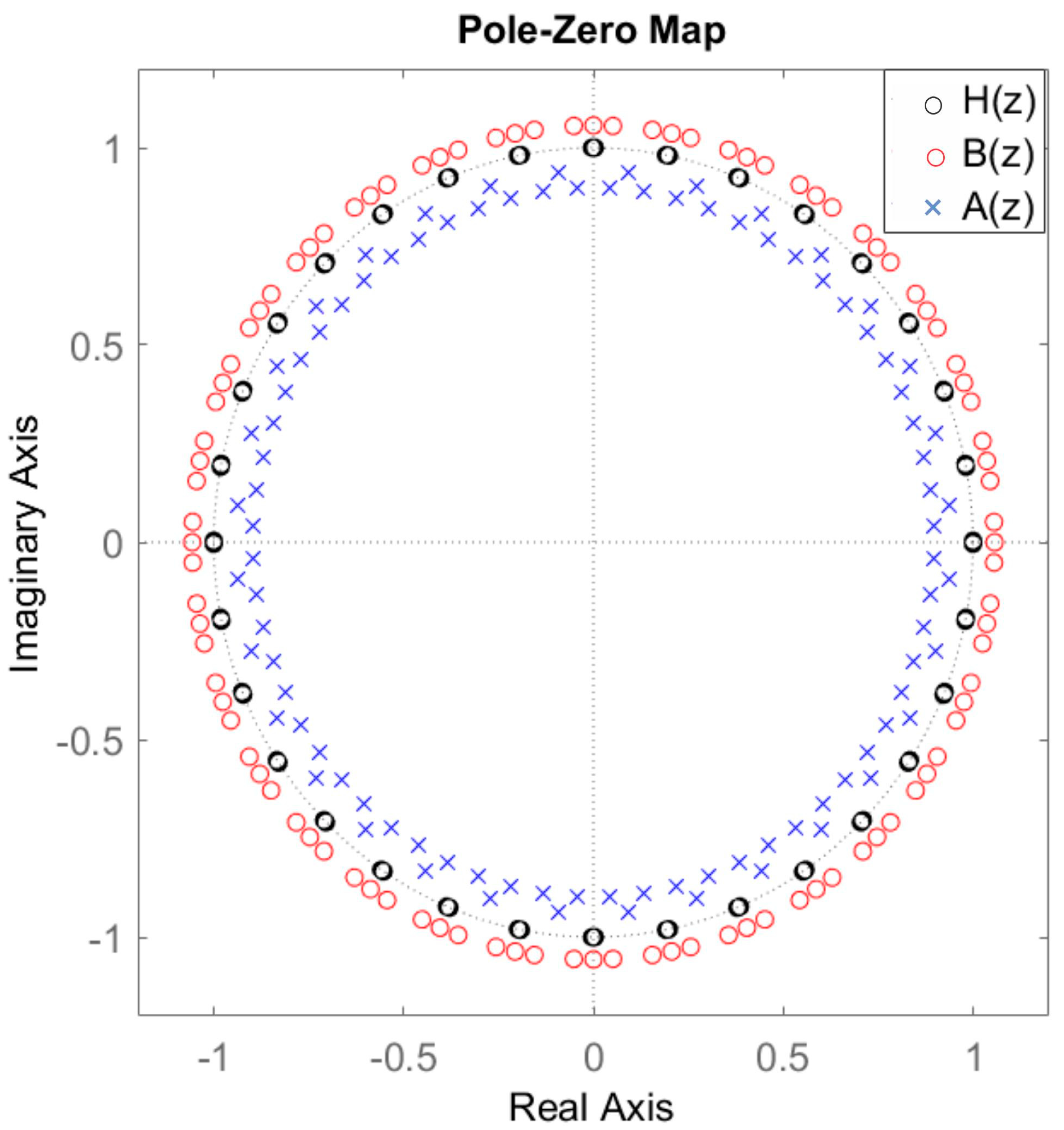
2.5. Stability Constraint
2.6. Constrained Linear Least-Squares (CLLS) Model
2.7. Linear Programming (LP) Model
2.8. Resonators’ Gains Calculation
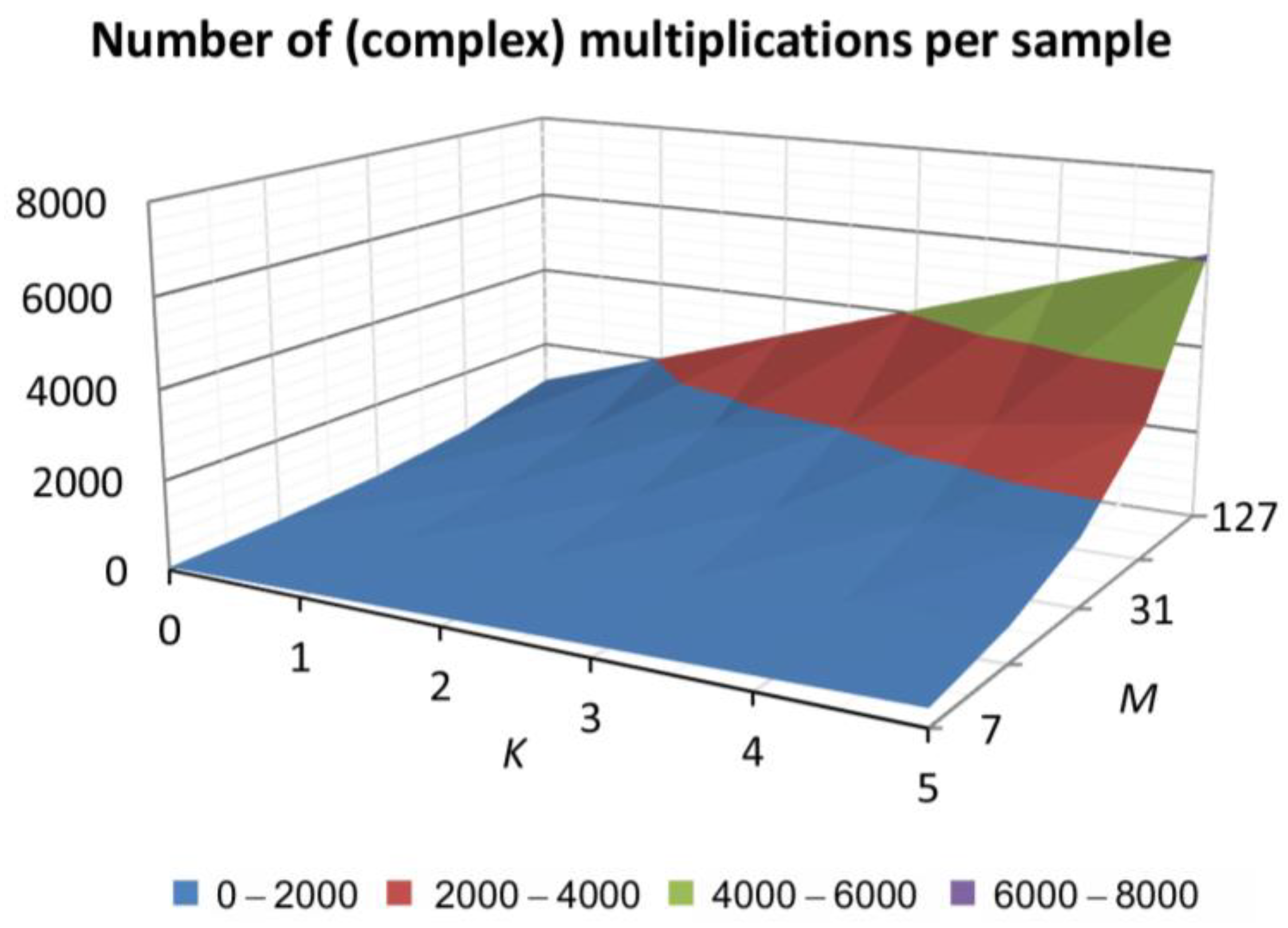
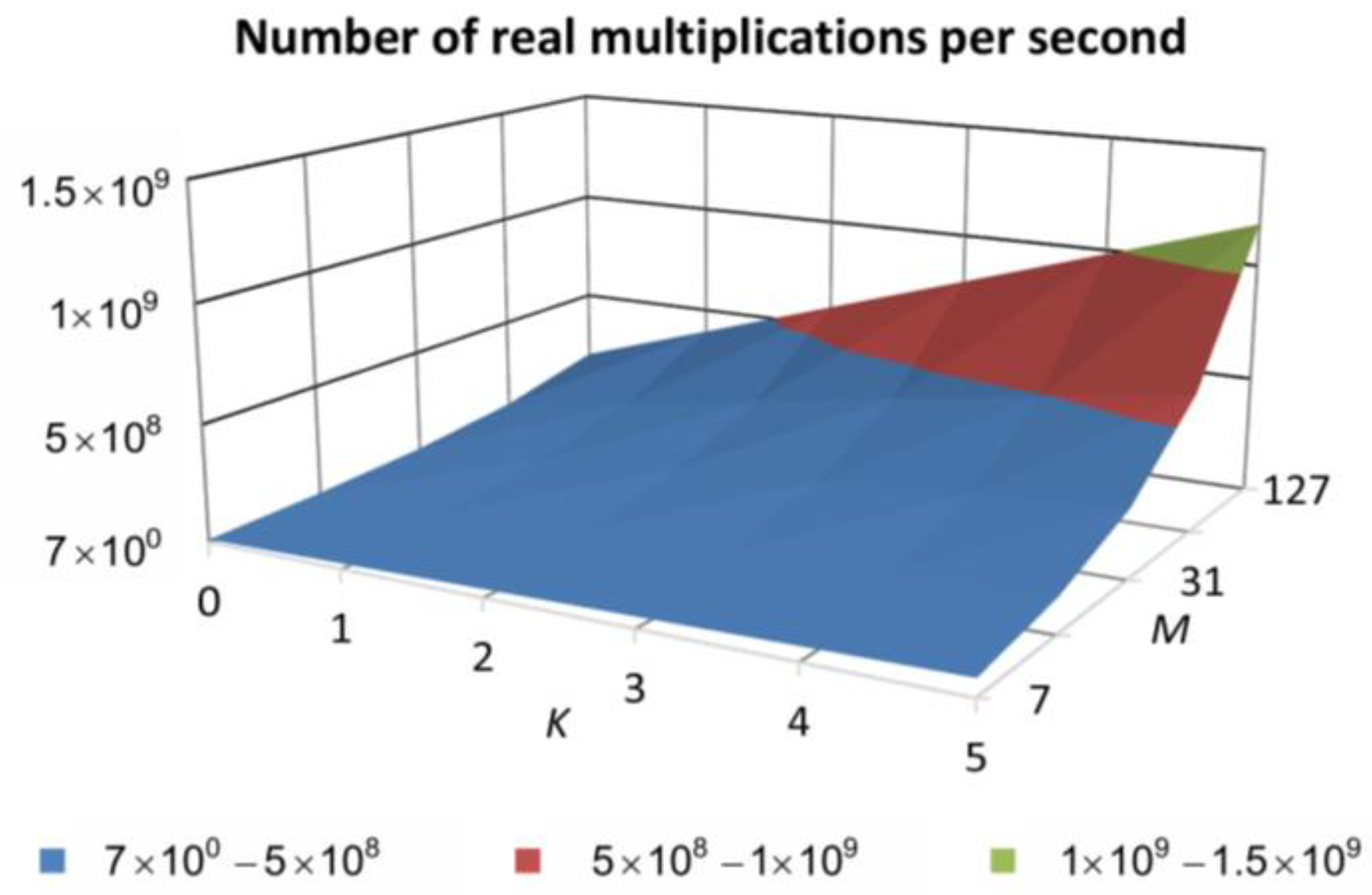
3. Computational Complexity
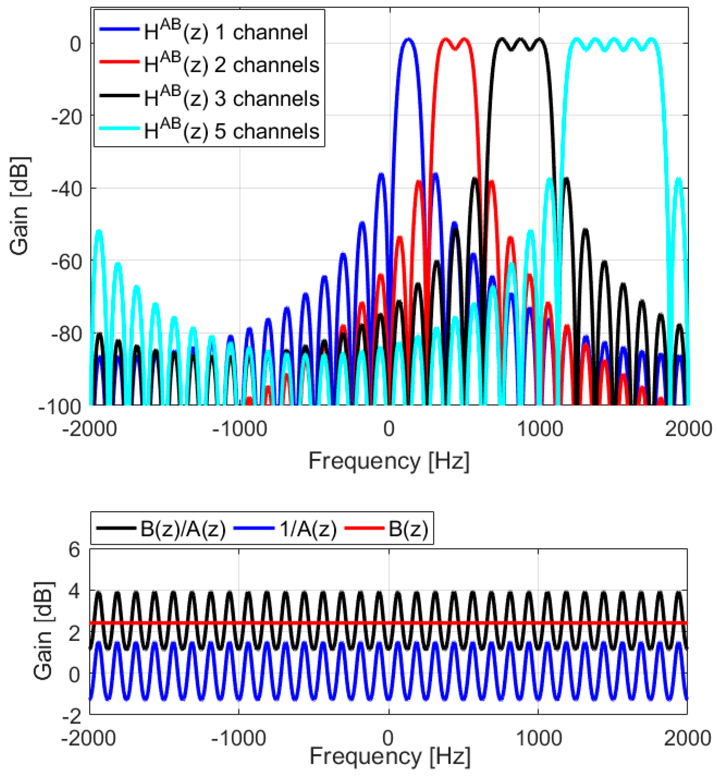
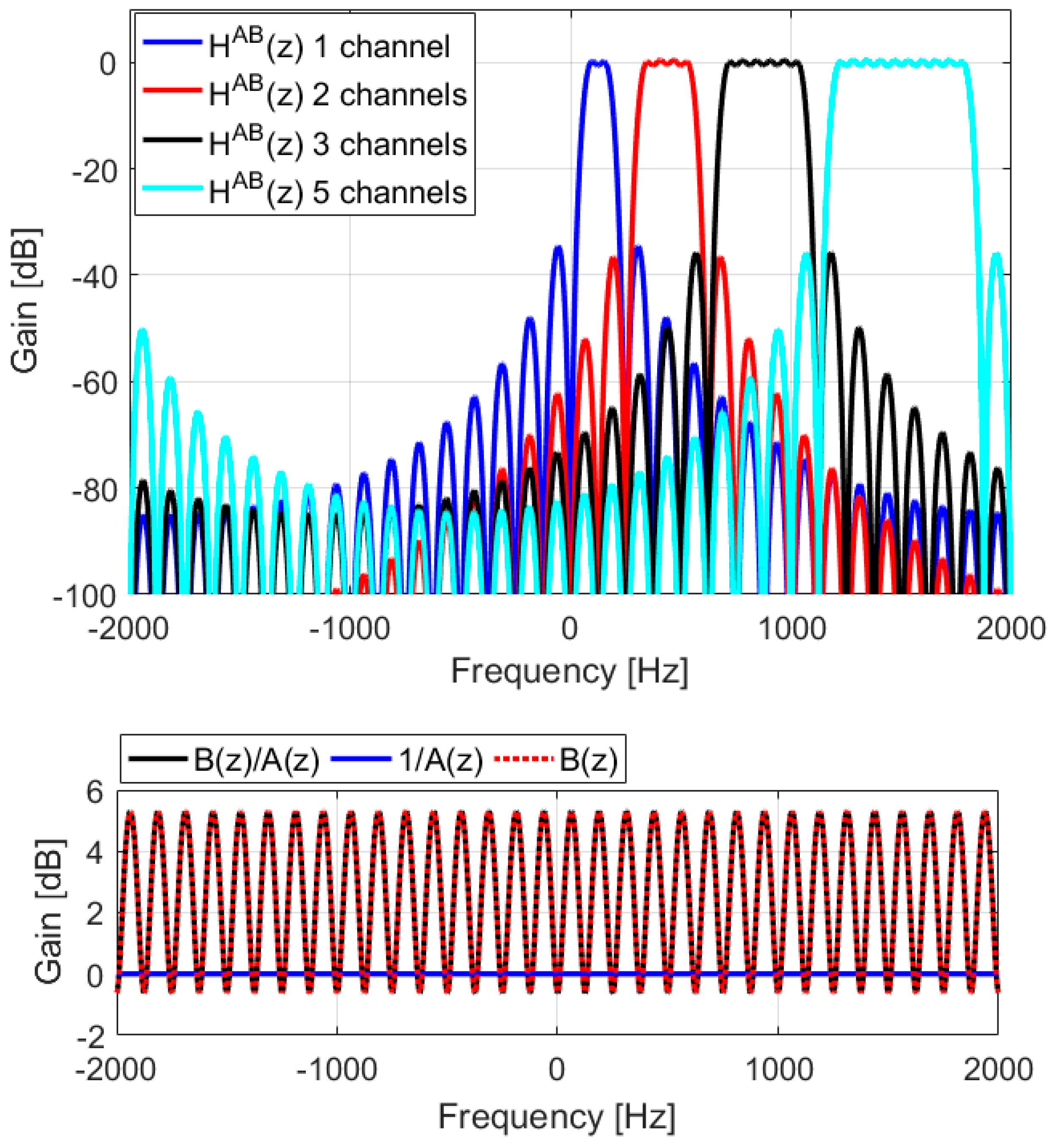
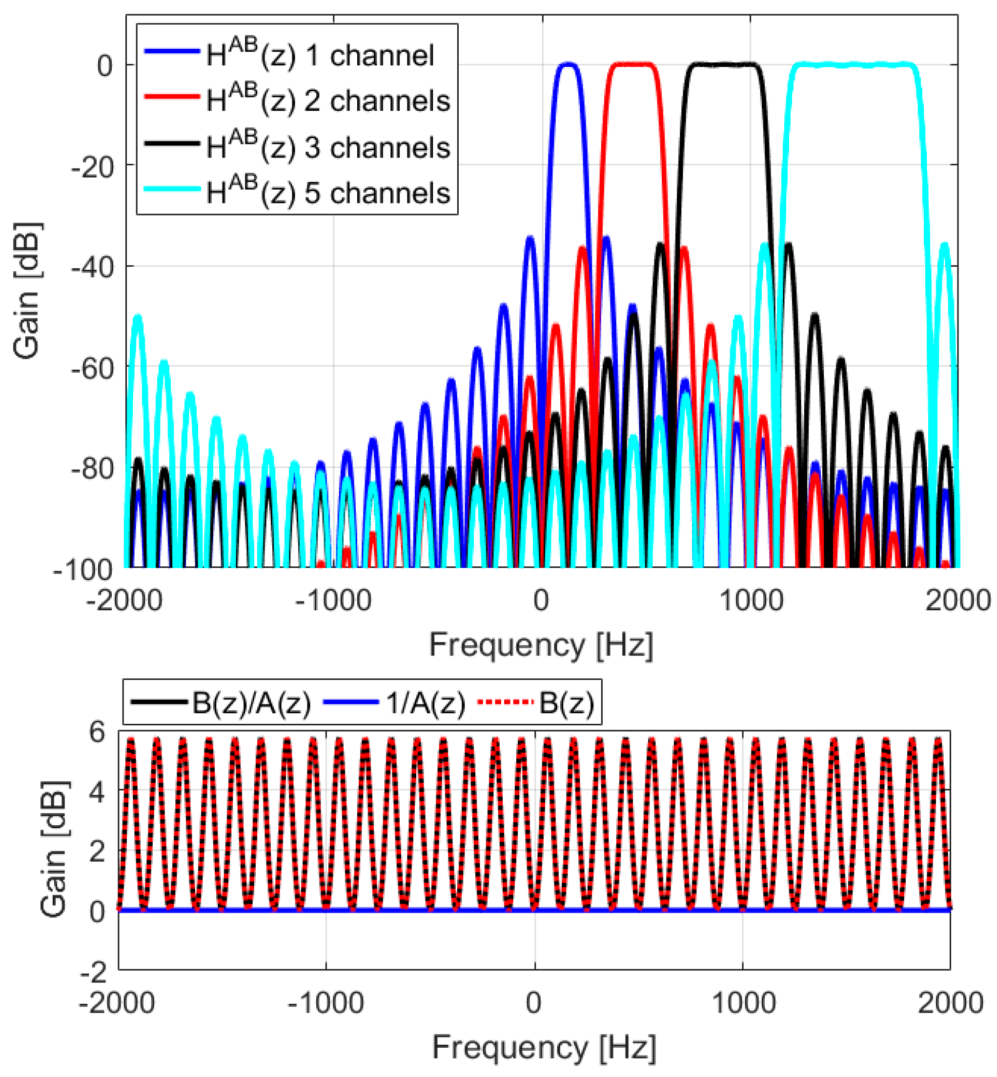
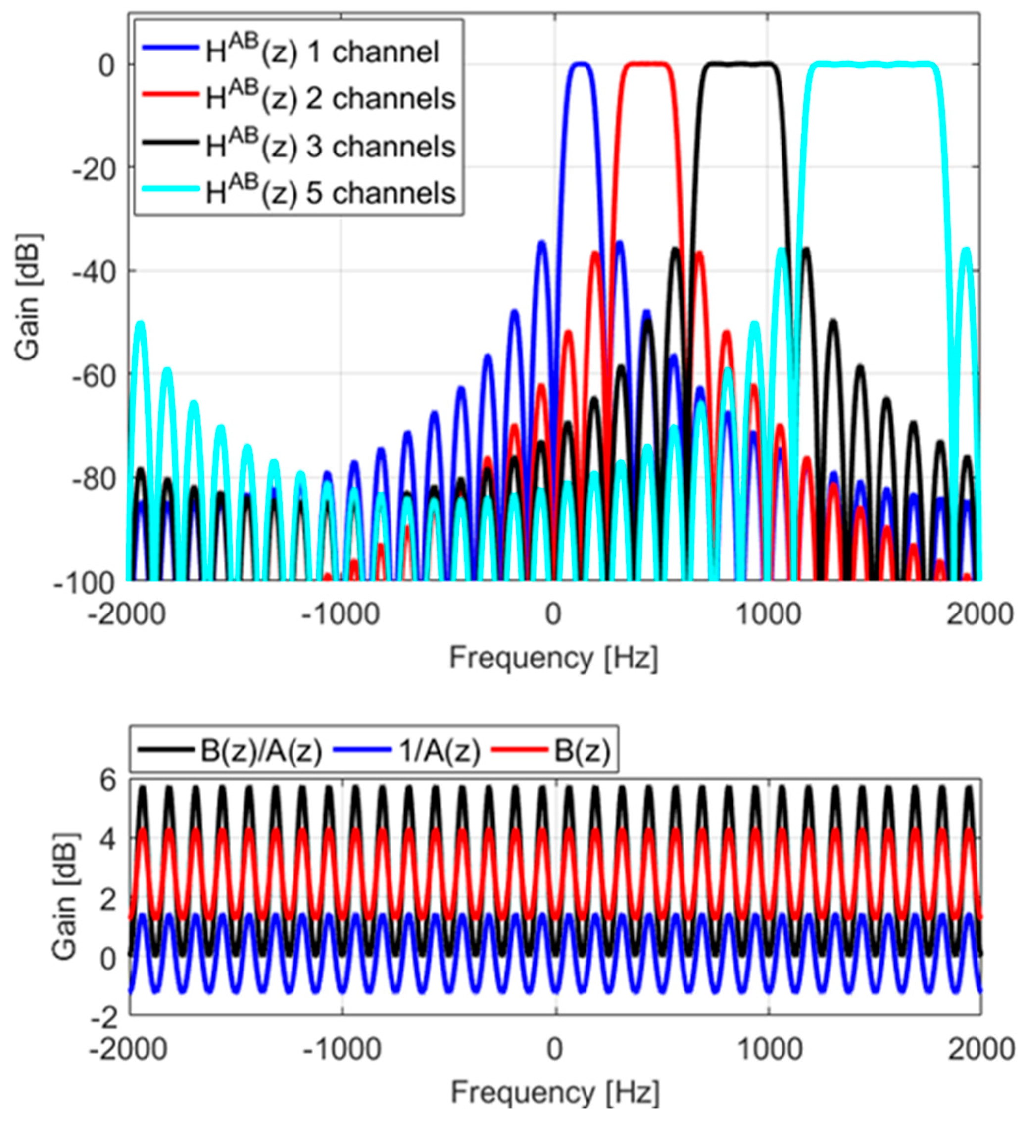
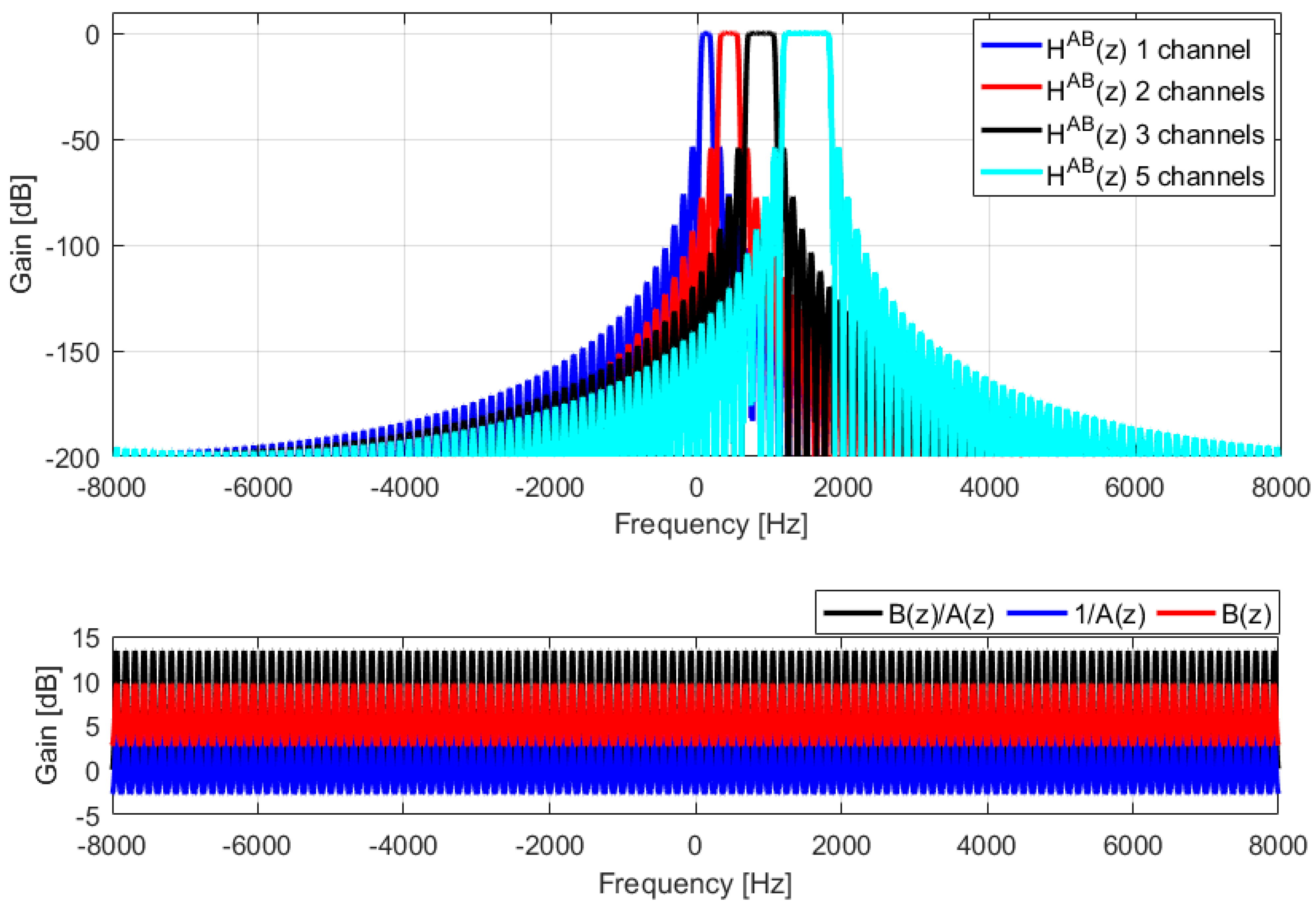
4. Design Examples
5. Suitable Applications of Described Filter Banks
5.1. Speech Signal Analysis and Speech and Speaker Recognition
5.2. Fine Audiogram Measurement and Hearing Correction
6. Conclusions
Author Contributions
Funding
Institutional Review Board Statement
Informed Consent Statement
Data Availability Statement
Conflicts of Interest
References
- Sarangi, S.; Sahidullah, M.; Saha, G. Optimization of Data-Driven Filterbank for Automatic Speaker Verification. Digit. Signal Process. 2020, 104, 102795. [Google Scholar] [CrossRef]
- Meerkoetter, K.; Ochs, K. A New Digital Equalizer Based on Complex Signal Processing; CSDSP’98: Sheffield, UK, 1998. [Google Scholar]
- Ikehara, M.; Takahashi, S. Design of Multirate Bandpass Digital Filters with Complex Coefficients. Electron. Commun. Jpn. (Part I Commun.) 1988, 71, 21–29. [Google Scholar] [CrossRef]
- Nikolova, Z.; Iliev, G.; Ovtcharov, M.; Poulkov, V. Complex Digital Signal Processing in Telecommunications. In Applications of Digital Signal Processing; IntechOpen: London, UK, 2011. [Google Scholar] [CrossRef]
- Iliev, G.; Nikolova, Z.; Poulkov, V.; Stoyanov, G. Noise Cancellation in OFDM Systems Using Adaptive Complex Narrowband IIR Filtering. In Proceedings of the IEEE International Conference on Communications, Istanbul, Turkey, 11–15 June 2006; Volume 6. [Google Scholar] [CrossRef]
- Kompis, M.; Kurz, A.; Pfiffner, F.; Senn, P.; Arnold, A.; Caversaccio, M. Is Complex Signal Processing for Bone Conduction Hearing Aids Useful? Cochlear Implant. Int. 2014, 15, S47–S50. [Google Scholar] [CrossRef] [PubMed]
- Park, K.-C.; Yoon, J.R. Performance Evaluation of the Complex-Coefficient Adaptive Equalizer Using the Hilbert Transform. J. Inf. Commun. Converg. Eng. 2016, 14, 78–83. [Google Scholar] [CrossRef]
- Nikolić, S.; Stančić, G.; Cvetković, S. Realization of Digital Filters with Complex Coefficients. Facta Univ. Ser. Autom. Control. Robot. 2018, 17, 25–38. [Google Scholar] [CrossRef]
- Padmanabhan, M.; Martin, K. Feedback-Based Orthogonal Digital Filters. IEEE Trans. Circuits Syst. II Analog. Digit. Signal Process. 1993, 40, 512–525. [Google Scholar] [CrossRef]
- Padmanabhan, M.; Martin, K. Resonator-Based Filter-Banks for Frequency-Domain Applications. IEEE Trans. Circuits Syst. 1991, 38, 1145–1159. [Google Scholar] [CrossRef]
- Zhang, G.; McGee, W.F. Windowing Techniques in the Design of Resonator Based Frequency Interpolation Filter Banks. In Proceedings of the ICASSP 91: 1991 International Conference on Acoustics, Speech, and Signal Processing, Toronto, ON, Canada, 14–17 April 1991; Volume 3. [Google Scholar] [CrossRef]
- Kusljevic, M.D.; Tomic, J.J. Multiple-Resonator-Based Power System Taylor-Fourier Harmonic Analysis. IEEE Trans. Instrum. Meas. 2015, 64, 554–563. [Google Scholar] [CrossRef]
- Peceli, G.; Simon, G. Generalization of the Frequency Sampling Method. In Proceedings of the IEEE Instrumentation and Measurement Technology Conference, Brussels, Belgium, 4–6 June 1996; pp. 339–343. [Google Scholar] [CrossRef]
- Kušljević, M.D. Quasi Multiple-Resonator-Based Harmonic Analysis. Measurement 2016, 94, 471–473. [Google Scholar] [CrossRef]
- Korać, V.Z.; Kušljević, M.D. Cascaded-Dispersed-Resonator-Based Off-Nominal-Frequency Harmonics Filtering. IEEE Trans. Instrum. Meas. 2021, 70, 1–3. [Google Scholar] [CrossRef]
- Kušljević, M.D. IIR Cascaded-Resonator-Based Filter Design for Recursive Frequency Analysis. IEEE Trans. Circuits Syst. II Express Briefs 2022, 69, 3939–3943. [Google Scholar] [CrossRef]
- Platas-Garza, M.A.; De La O Serna, J.A. Dynamic Harmonic Analysis through Taylor-Fourier Transform. IEEE Trans. Instrum. Meas. 2011, 60, 804–813. [Google Scholar] [CrossRef]
- Kušljević, M.D. Adaptive Resonator-Based Method for Power System Harmonic Analysis. IET Sci. Meas. Technol. 2008, 2, 177–185. [Google Scholar] [CrossRef]
- Tseng, C.C.; Lee, S.L. Minimax Design of Stable IIR Digital Filter with Prescribed Magnitude and Phase Responses. IEEE Trans. Circuits Syst. I Fundam. Theory Appl. 2002, 49, 547–551. [Google Scholar] [CrossRef]
- Tomic, J.J.; Poljak, P.D.; Kušljevic, M.D. Frequency-Response-Controlled Multiple-Resonator-Based Harmonic Analysis. Electron. Lett. 2018, 54, 202–204. [Google Scholar] [CrossRef]
- Kušljević, M.D.; Vujičić, V.V. Design of Digital Constrained Linear Least-Squares Multiple-Resonator-Based Harmonic Filtering. Acoustics 2022, 2022, 111–122. [Google Scholar] [CrossRef]
- Chen, X.; Parks, T.W. Design of FIR Filters in the Complex Domain. IEEE Trans. Acoust. Speech Signal Process. 1987, 35, 144–153. [Google Scholar] [CrossRef]
- Lang, M.C. Least-Squares Design of IIR Filters with Prescribed Magnitude and Phase Responses and a Pole Radius Constraint. IEEE Trans. Signal Process. 2000, 48, 3109–3121. [Google Scholar] [CrossRef]
- Kušljević, M.D. Cascaded-Resonator-Based Recursive Harmonic Analysis. In Fourier Transform and Its Generalizations [Working Title]; IntechOpen: London, UK, 2022. [Google Scholar]


| = 7 | = 15 | = 31 | = 63 | = 127 | |
|---|---|---|---|---|---|
| 0 | 64 | 128 | 256 | 512 | 1024 |
| 1 | 128 | 256 | 512 | 1024 | 2048 |
| 2 | 192 | 384 | 768 | 1536 | 3072 |
| 3 | 256 | 512 | 1024 | 2048 | 4096 |
| 4 | 320 | 640 | 1280 | 2560 | 5120 |
| 5 | 384 | 768 | 1536 | 3072 | 6144 |
| = 7 | = 15 | = 31 | = 63 | = 127 | |
|---|---|---|---|---|---|
| 0 | |||||
| 1 | |||||
| 2 | |||||
| 3 | |||||
| 4 | |||||
| 5 |
Disclaimer/Publisher’s Note: The statements, opinions and data contained in all publications are solely those of the individual author(s) and contributor(s) and not of MDPI and/or the editor(s). MDPI and/or the editor(s) disclaim responsibility for any injury to people or property resulting from any ideas, methods, instructions or products referred to in the content. |
© 2023 by the authors. Licensee MDPI, Basel, Switzerland. This article is an open access article distributed under the terms and conditions of the Creative Commons Attribution (CC BY) license (https://creativecommons.org/licenses/by/4.0/).
Share and Cite
Kušljević, M.D.; Vujičić, V.V.; Tomić, J.J.; Poljak, P.D. IIR Cascaded-Resonator-Based Complex Filter Banks. Acoustics 2023, 5, 535-552. https://doi.org/10.3390/acoustics5020032
Kušljević MD, Vujičić VV, Tomić JJ, Poljak PD. IIR Cascaded-Resonator-Based Complex Filter Banks. Acoustics. 2023; 5(2):535-552. https://doi.org/10.3390/acoustics5020032
Chicago/Turabian StyleKušljević, Miodrag D., Vladimir V. Vujičić, Josif J. Tomić, and Predrag D. Poljak. 2023. "IIR Cascaded-Resonator-Based Complex Filter Banks" Acoustics 5, no. 2: 535-552. https://doi.org/10.3390/acoustics5020032