

Automatic CHIEF Point Selection for Finite Element–Boundary Element Acoustic Backscattering †

Abstract
:1. Introduction
2. Methods
2.1. Exterior Acoustic Problem
2.2. The Non-Uniqueness of Solutions: CHIEF
2.3. Automatic Selection of CHIEF Points
| Algorithm 1 Algorithm Find-CHIEF-points |
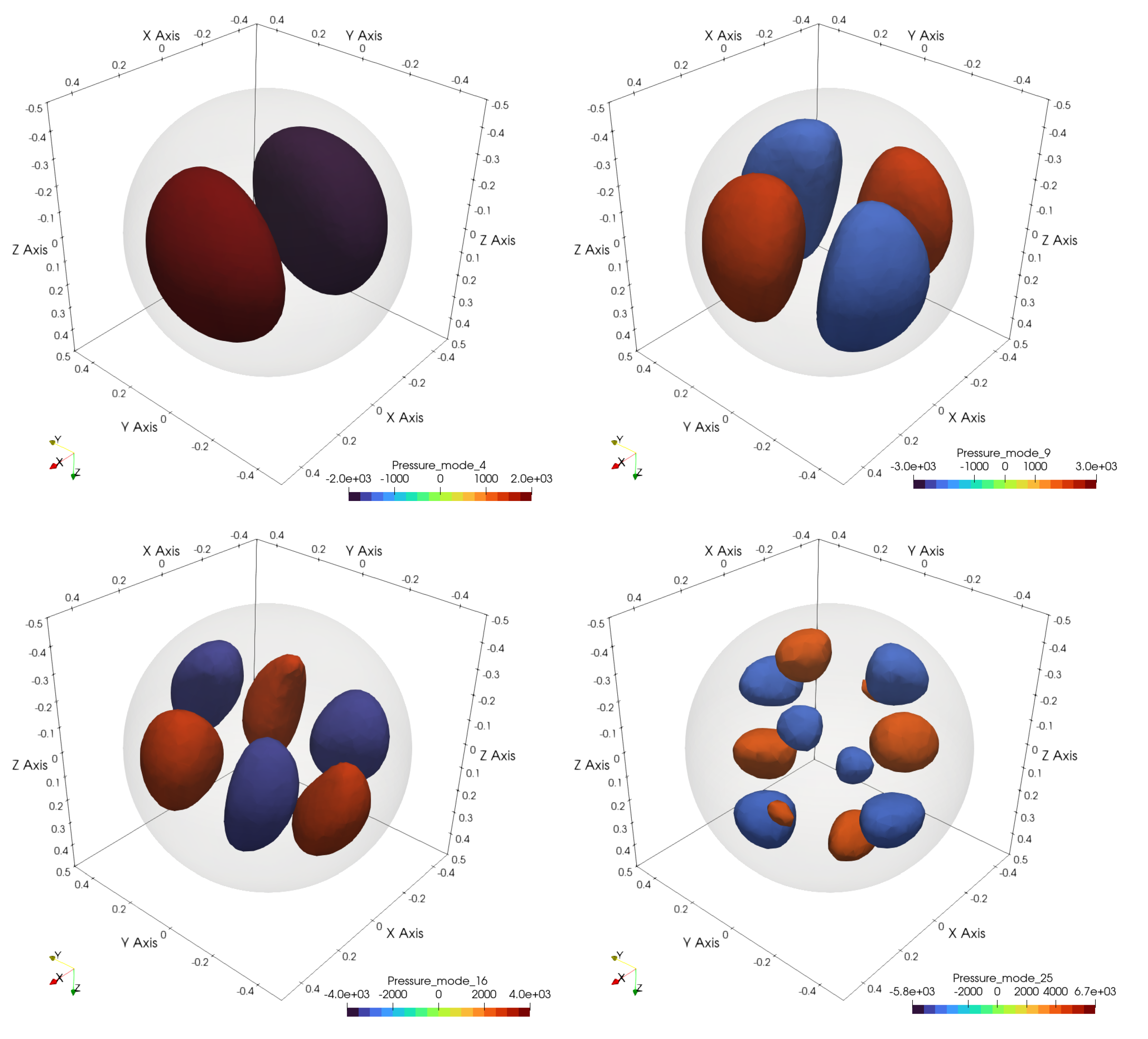
Require: Solution of the interior modal problem for number of modes Make the set of interior points, I, initially empty for do ▹ For all pressure modes Compute the magnitude of the pressure mode: . Compute threshold . Collect finite elements connected to nodes j with nodal dofs into a set E. while E is not empty do Mark the subset S of E such that all such elements are connected together Find all nodes connected by elements from the set S, adding them into a set N. Add the node with the largest value within the set N to the set I. Remove the elements of S from E end while end for return
I |
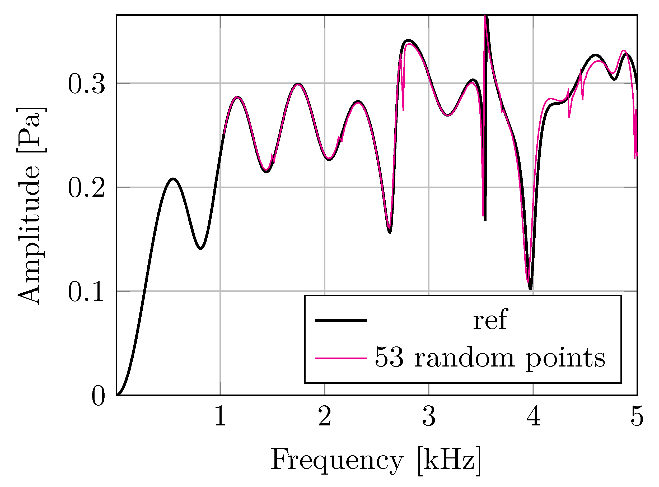
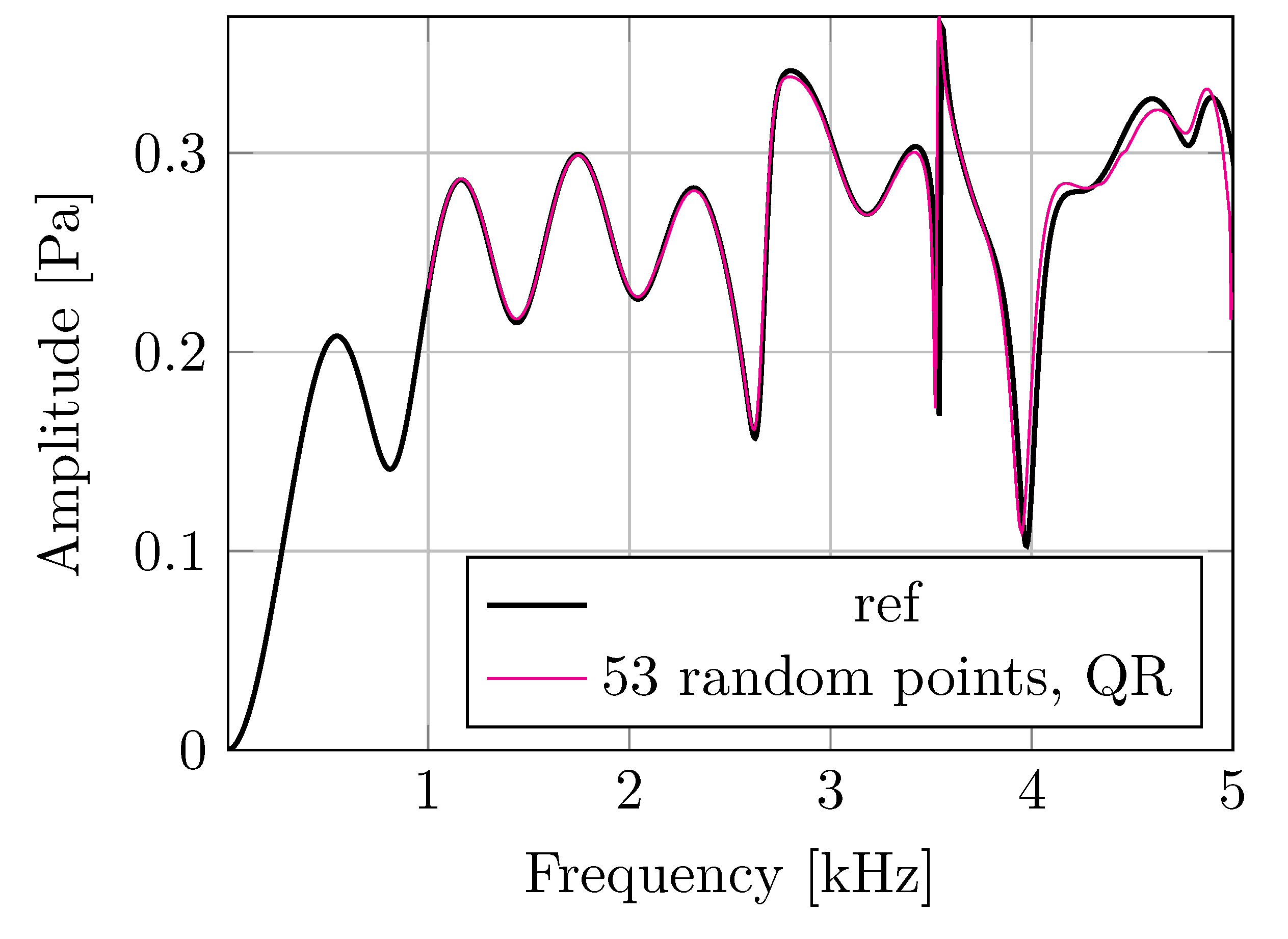
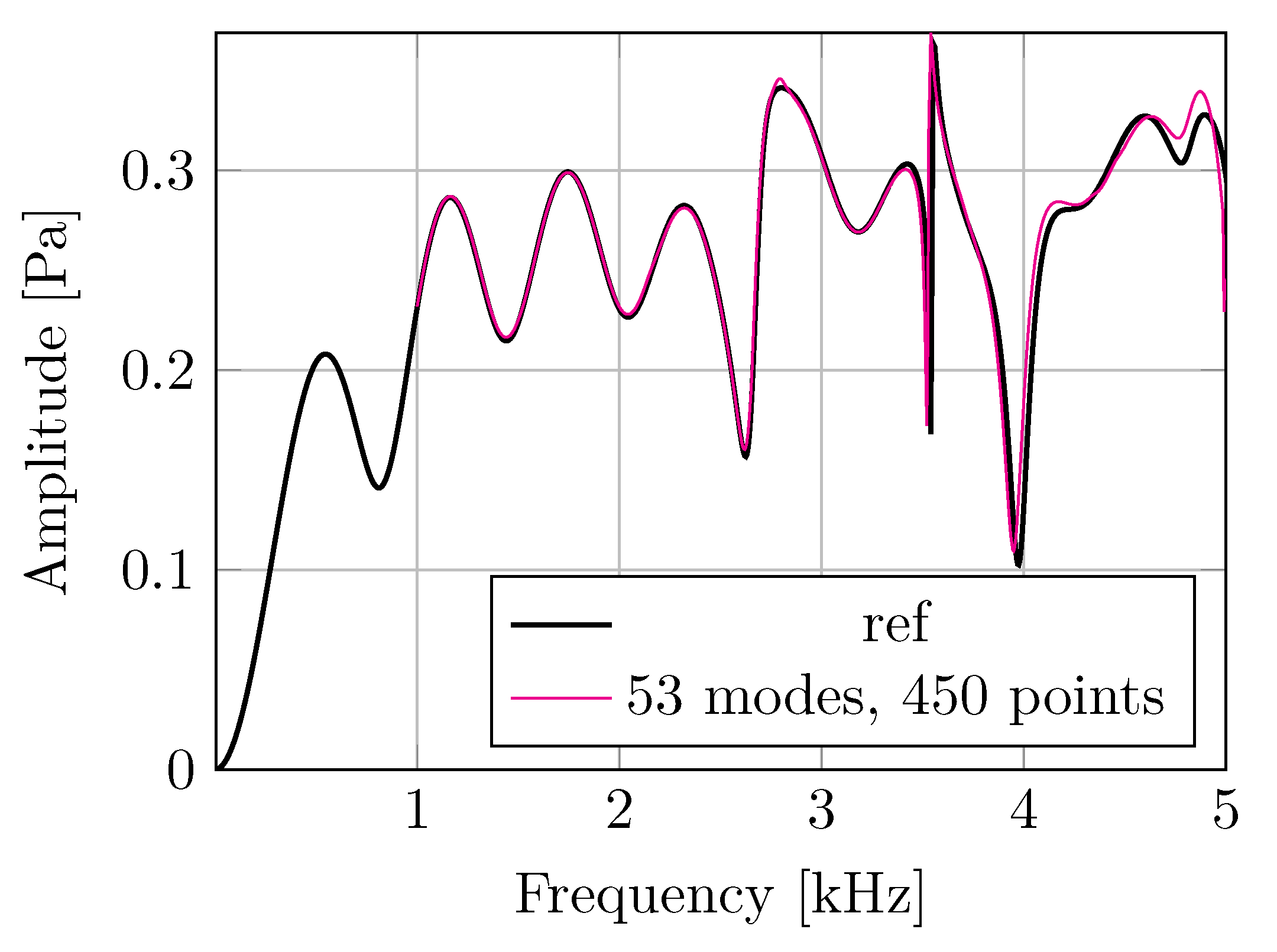
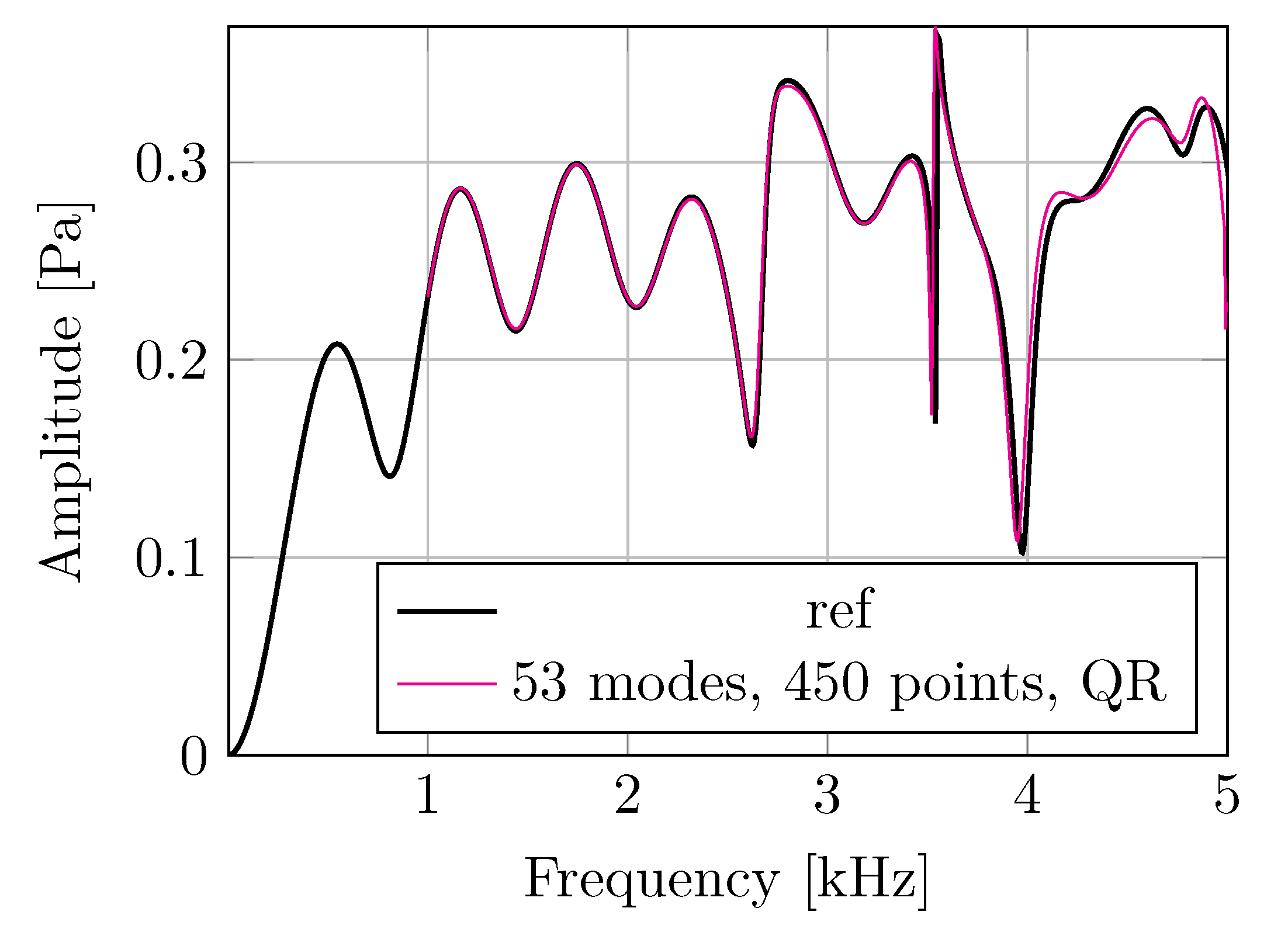
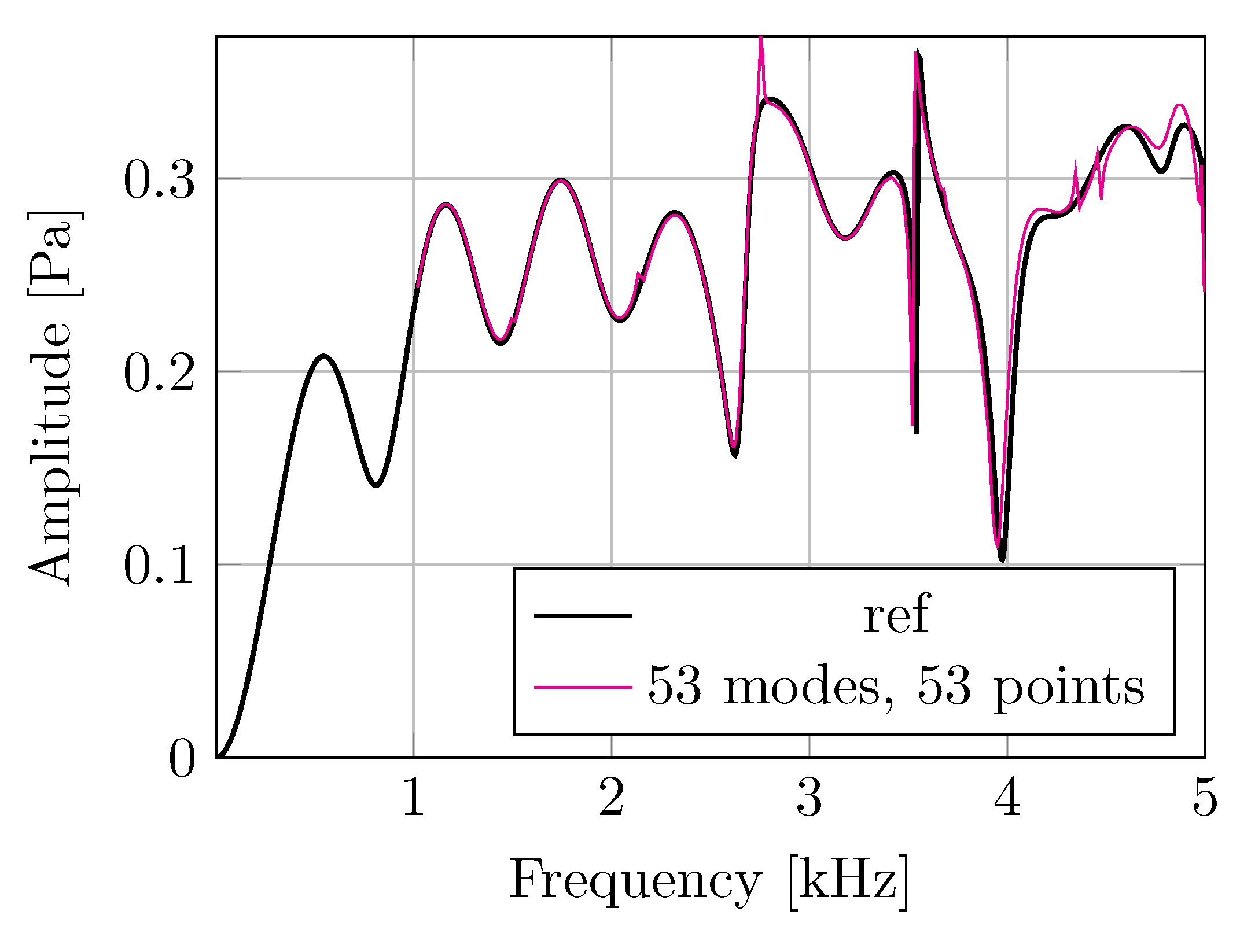
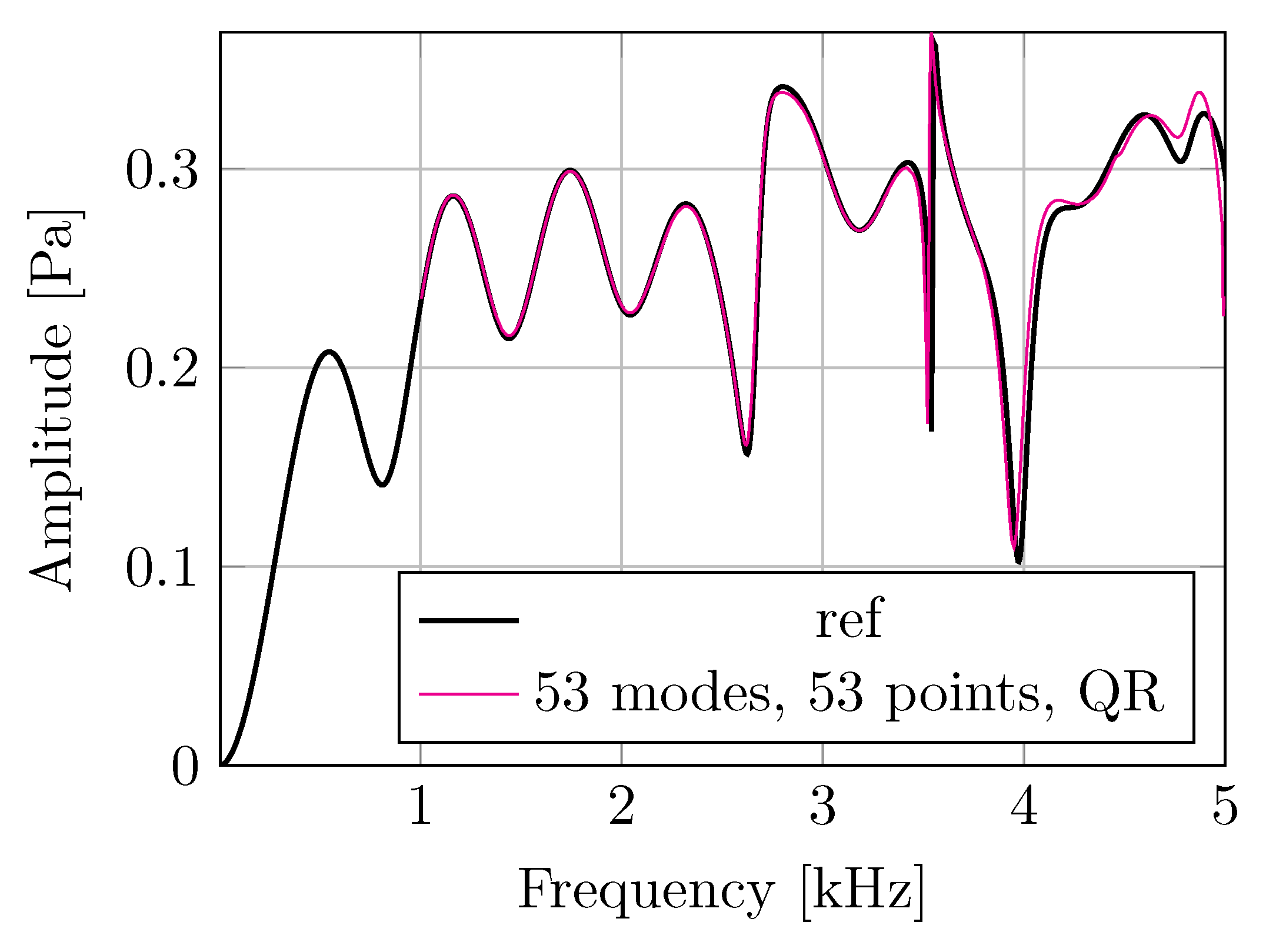
3. Results
4. Discussion
5. Conclusions
Author Contributions
Funding
Data Availability Statement
Acknowledgments
Conflicts of Interest
References
- Junger, M. Acoustic fluid-elastic structure interactions: Basic concepts. Comput. Struct. 1997, 65, 287–293. [Google Scholar] [CrossRef]
- Hackman, R.H. Acoustic Scattering from Elastic Solids. In Physical Acoustics; Pierce, A.D., Thurston, R., Eds.; Physical Acoustics; Academic Press: Cambridge, MA, USA, 1993; Volume 22, pp. 1–194. [Google Scholar] [CrossRef]
- Harari, I.; Grosh, K.; Hughes, T.J.R.; Malhotra, M.; Pinsky, P.M.; Stewart, J.R.; Thompson, L.L. Recent developments in finite element methods for structural acoustics. Arch. Comput. Methods Eng. 1996, 3, 131–309. [Google Scholar] [CrossRef]
- Kirkup, S. The Boundary Element Method in Acoustics: A Survey. Appl. Sci. 2019, 9, 1642. [Google Scholar] [CrossRef]
- Amini, S.; Harris, P. A comparison between various boundary integral formulations of the exterior acoustic problem. Comput. Methods Appl. Mech. Eng. 1990, 84, 59–75. [Google Scholar] [CrossRef]
- Copley, L.G. Fundamental Results Concerning Integral Representations in Acoustic Radiation. J. Acoust. Soc. Am. 1968, 44, 28–32. [Google Scholar] [CrossRef]
- Schenck, H.A. Improved Integral Formulation for Acoustic Radiation Problems. J. Acoust. Soc. Am. 1968, 44, 41–58. [Google Scholar] [CrossRef]
- Wilton, D.T. Acoustic radiation and scattering from elastic structures. Int. J. Numer. Methods Eng. 1978, 13, 123–138. [Google Scholar] [CrossRef]
- Seybert, A. A note on methods for circumventing non-uniqueness when using integral equations. J. Sound Vib. 1987, 115, 171–172. [Google Scholar] [CrossRef]
- Kirkup, S. The influence of the weighting parameter on the improved boundary element solution of the exterior Helmholtz equation. Wave Motion 1992, 15, 93–101. [Google Scholar] [CrossRef]
- Benthien, W.; Schenck, A. Nonexistence and nonuniqueness problems associated with integral equation methods in acoustics. Comput. Struct. 1997, 65, 295–305. [Google Scholar] [CrossRef]
- Benthien, G.W.; Schenck, H.A. Structural-Acoustic Coupling. In Boundary Element Methods in Acoustics; Springer: New York, NY, USA, 1977; pp. 109–128. [Google Scholar]
- Krysl, P. Citations of the Schenk 1968 CHIEF Paper. Available online: https://asa.scitation.org/doi/citedby/10.1121/1.1911085 (accessed on 6 April 2023).
- Seybert, A.F.; Rengarajan, T.K. The use of CHIEF to obtain unique solutions for acoustic radiation using boundary integral equations. J. Acoust. Soc. Am. 1987, 81, 1299–1306. [Google Scholar] [CrossRef]
- Segalman, D.J.; Lobitz, D.W. SuperCHIEF: A Modified CHIEF Method. In Boundary Element Technology VII; Brebbia, C.A., Ingber, M.S., Eds.; Springer: Dordrecht, The Netherlands, 1992; pp. 511–528. [Google Scholar] [CrossRef]
- Wu, T.W.; Seybert, A.F. A weighted residual formulation for the CHIEF method in acoustics. J. Acoust. Soc. Am. 1991, 90, 1608–1614. [Google Scholar] [CrossRef]
- Wu, T.W.; Jia, Z.H. A Choice of Practical Approaches to Overcome the Nonuniqueness Problem of the BEM in Acoustic Radiation and Scattering. In Boundary Element Technology VII; Brebbia, C.A., Ingber, M.S., Eds.; Springer: Dordrecht, The Netherlands, 1992; pp. 501–510. [Google Scholar] [CrossRef]
- Provatidis, C.G.; Zafiropoulos, N.K. On the ‘interior Helmholtz integral equation formulation’ in sound radiation problems. Eng. Anal. Bound. Elem. 2002, 26, 29–40. [Google Scholar] [CrossRef]
- Lee, J.W.; Chen, J.T.; Nien, C.F. Indirect boundary element method combining extra fundamental solutions for solving exterior acoustic problems with fictitious frequencies. J. Acoust. Soc. Am. 2019, 145, 3116–3132. [Google Scholar] [CrossRef] [PubMed]
- Kleefeld, A.; Lin, T.C. A Global Galerkin Method for Solving the Exterior Neumann Problem for the Helmholtz Equation Using Panich’s Integral Equation Approach. SIAM J. Sci. Comput. 2013, 35, A1709–A1735. [Google Scholar] [CrossRef]
- Bartolozzi, G.; D’Amico, R.; Pratellesi, A.; Pierini, M. An Efficient Method for Selecting CHIEF Points. In Proceedings of the International Conference on Structural Dynamics, EURODYN 2011, Leuven, Belgium, 4–6 July 2011. [Google Scholar]
- Wang, X.; Chen, H.; Zhang, J. An efficient boundary integral equation method for multi-frequency acoustics analysis. Eng. Anal. Bound. Elem. 2015, 61, 282–286. [Google Scholar] [CrossRef]
- Marburg, S.; Wu, T.W. Treating the Phenomenon of Irregular Frequencies. In Computational Acoustics of Noise Propagation in Fluids—Finite and Boundary Element Methods; Springer: Berlin/Heidelberg, Germany, 2008; pp. 411–434. [Google Scholar] [CrossRef]
- Burton, A.J.; Miller, G.F.; Wilkinson, J.H. The application of integral equation methods to the numerical solution of some exterior boundary-value problems. Proc. R. Soc. Lond. A Math. Phys. Sci. 1971, 323, 201–210. [Google Scholar] [CrossRef]
- Mohsen, A.; Hesham, M. An efficient method for solving the nonuniqueness problem in acoustic scattering. Commun. Numer. Methods Eng. 2006, 22, 1067–1076. [Google Scholar] [CrossRef]
- Liu, Y. On the BEM for acoustic wave problems. Eng. Anal. Bound. Elem. 2019, 107, 53–62. [Google Scholar] [CrossRef]
- Atalla, N.; Sgard, F. Finite Element and Boundary Methods in Structural Acoustics and Vibration; Imprint CRC Press: Boca Raton, FL, USA, 2015. [Google Scholar]
- Sivapuram, R.; Krysl, P. On the energy-sampling stabilization of Nodally Integrated Continuum Elements for dynamic analyses. Finite Elem. Anal. Des. 2019, 167, 103322. [Google Scholar] [CrossRef]
- Kirkup, S.M. The Boundary Element Method in Acoustics: A Development in Fortran; Integrated Sound Software: Hebden Bridge, UK, 1998. [Google Scholar]
- Rezayat, M.; Shippy, D.; Rizzo, F. On time-harmonic elastic-wave analysis by the boundary element method for moderate to high frequencies. Comput. Methods Appl. Mech. Eng. 1986, 55, 349–367. [Google Scholar] [CrossRef]
- Rosen, E.M.; Canning, F.X.; Couchman, L.S. A sparse integral equation method for acoustic scattering. J. Acoust. Soc. Am. 1995, 98, 599–610. [Google Scholar] [CrossRef]
- Sung, S.H.; Nefske, D.J. Structural-Acoustic Finite-Element Analysis for Interior Acoustics. In Engineering Vibroacoustic Analysis; John Wiley & Sons, Ltd.: Hoboken, NJ, USA, 2016; Chapter 6; pp. 144–178. [Google Scholar] [CrossRef]
- The Julia Project. The Julia Programming Language. Available online: https://julialang.org/ (accessed on 13 March 2023).
- Bezanson, J.; Edelman, A.; Karpinski, S.; Shah, V.B. Julia: A fresh approach to numerical computing. SIAM Rev. 2017, 59, 65–98. [Google Scholar] [CrossRef]
- Petr Krysl. FinEtools: Finite Element Tools in Julia. Available online: https://github.com/PetrKryslUCSD/FinEtools.jl (accessed on 13 March 2021).
- Krysl, P.; Sivapuram, R.; Abawi, A.T. Rapid free-vibration analysis with model reduction based on coherent nodal clusters. Int. J. Numer. Methods Eng. 2020, 121, 3274–3299. [Google Scholar] [CrossRef]
- Abawi, A.T.; Krysl, P. Coupled finite element/boundary element formulation for scattering from axially-symmetric objects in three dimensions. J. Acoust. Soc. Am. 2017, 142, 3637. [Google Scholar] [CrossRef]


| Multiplicity | Interior Natural Frequency [Hz] | ||
|---|---|---|---|
| 1 | 1.50000 | 3.00000 | 4.50000 |
| 3 | 2.14544 | 3.68854 | 5.20633 |
| 5 | 2.75185 | 4.34255 | 5.88377 |
| 7 | 3.33649 | 4.97380 | 6.54032 |
| 9 | 3.90688 | 5.58868 | 7.18091 |
| 11 | 4.46707 | 6.19106 | 7.80880 |
Disclaimer/Publisher’s Note: The statements, opinions and data contained in all publications are solely those of the individual author(s) and contributor(s) and not of MDPI and/or the editor(s). MDPI and/or the editor(s) disclaim responsibility for any injury to people or property resulting from any ideas, methods, instructions or products referred to in the content. |
© 2023 by the authors. Licensee MDPI, Basel, Switzerland. This article is an open access article distributed under the terms and conditions of the Creative Commons Attribution (CC BY) license (https://creativecommons.org/licenses/by/4.0/).
Share and Cite
Krysl, P.; Abawi, A.T. Automatic CHIEF Point Selection for Finite Element–Boundary Element Acoustic Backscattering. Acoustics 2023, 5, 522-534. https://doi.org/10.3390/acoustics5020031
Krysl P, Abawi AT. Automatic CHIEF Point Selection for Finite Element–Boundary Element Acoustic Backscattering. Acoustics. 2023; 5(2):522-534. https://doi.org/10.3390/acoustics5020031
Chicago/Turabian StyleKrysl, Petr, and Ahmad T. Abawi. 2023. "Automatic CHIEF Point Selection for Finite Element–Boundary Element Acoustic Backscattering" Acoustics 5, no. 2: 522-534. https://doi.org/10.3390/acoustics5020031