
A Basic Study on the Design of Dotted-Art Heterogeneous MPP Sound Absorbers


Abstract
:1. Introduction
1.1. Background: Microperforated Panels (MPPs)
1.2. Heterogeneous MPPs and Design-Oriented MPPs
1.3. Outline of the Present Work
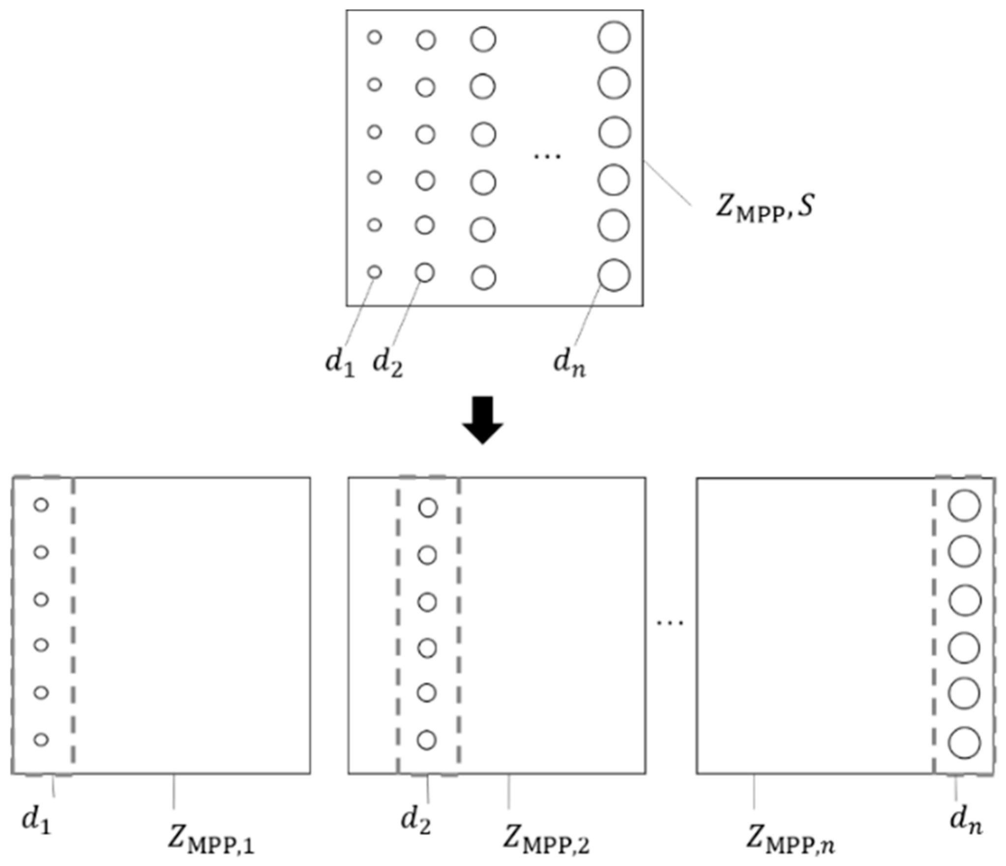
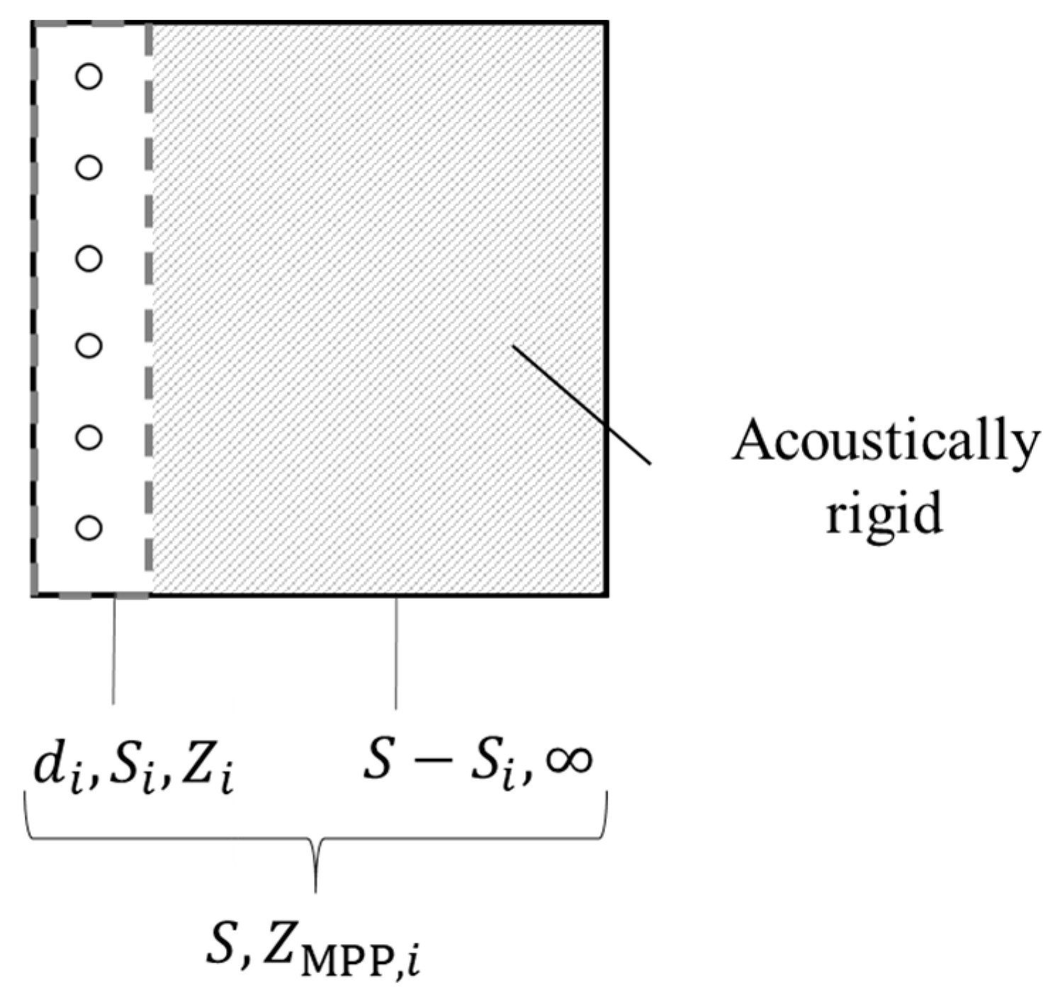
2. Prediction Method for the Absorption Characteristics of Heterogeneous MPPs
3. Preliminary Study: Applicability of the Synthetic Impedance Method to Various Heterogeneous MPPs
3.1. Experiment
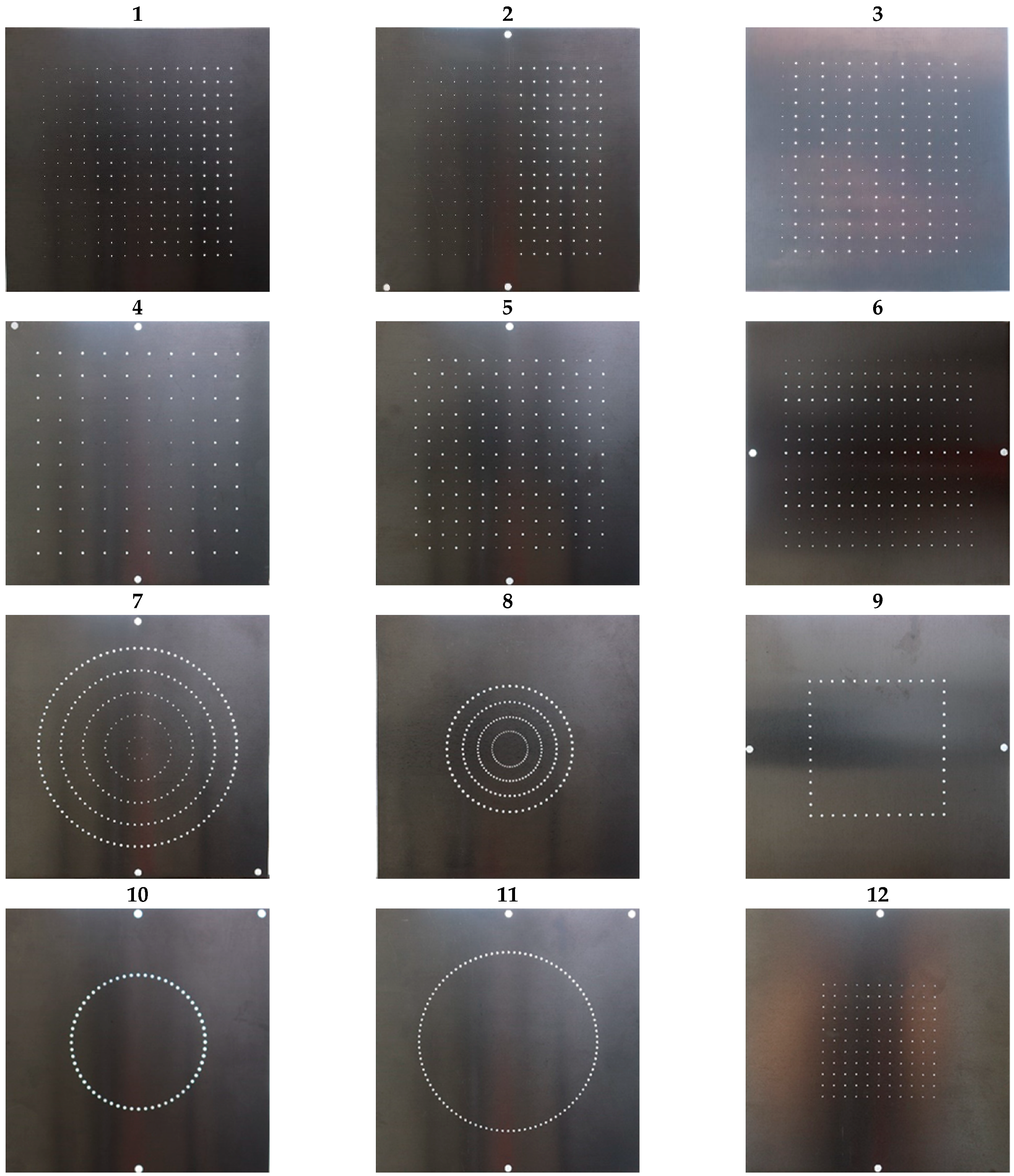
3.1.1. Specimens
- Specimen 1 consists of four types of holes with diameters of 0.3 mm, 0.5 mm, 0.7 mm, and 0.9 mm, which are arranged in a gradient pattern so that the holes become larger every four rows (due to the limitation of the specimen size, only the 0.9 mm holes are arranged into three rows).
- Specimen 2 consists of two types of holes with diameters of 0.3 mm and 0.9 mm, which are arranged in a solidified manner.
- Specimen 3 consists of two types of holes with diameters of 0.3 mm and 0.9 mm, which are arranged into alternating rows.
- Specimen 4 consists of holes with diameters of 0.3 mm, 0.5 mm, 0.7 mm, 0.9 mm, and 1.1 mm, which are arranged in increasing order from the inner side.
- Specimen 5 consists of two types of holes with diameters of 0.3 mm and 0.9 mm, which are arranged in a checkerboard pattern so that the different holes are adjacent to each other.
- Specimen 6 consists of four types of holes with diameters of 0.3 mm, 0.5 mm, 0.7 mm, and 0.9 mm, arranged into rows of one.
- Specimen 7 consists of five types of holes with diameters of 0.3 mm, 0.5 mm, 0.7 mm, 0.9 mm, and 1.1 mm, which are arranged on circumferences of 10 mm, 30 mm, 50 mm, 70 mm, and 90 mm, respectively, in order from the inside.
- Specimen 8 consists of four types of holes with diameters of 0.5 mm, 0.7 mm, 0.9 mm, and 1.1 mm, which are arranged on circumferences of 16 mm, 29 mm, 42.5 mm, and 57 mm, respectively, in order from the inner side.
- Specimen 9 consists of 1.0 mm diameter holes arranged on a square of 60 mm per side.
- Specimen 10 consists of 1.0 mm diameter holes arranged on a circumference of 60 mm.
- Specimen 11 consists of holes with a diameter of 1.0 mm arranged on a circumference of 80 mm.
- Specimen 12 consists of 0.5 mm diameter holes arranged in the central area of a 50 mm square.
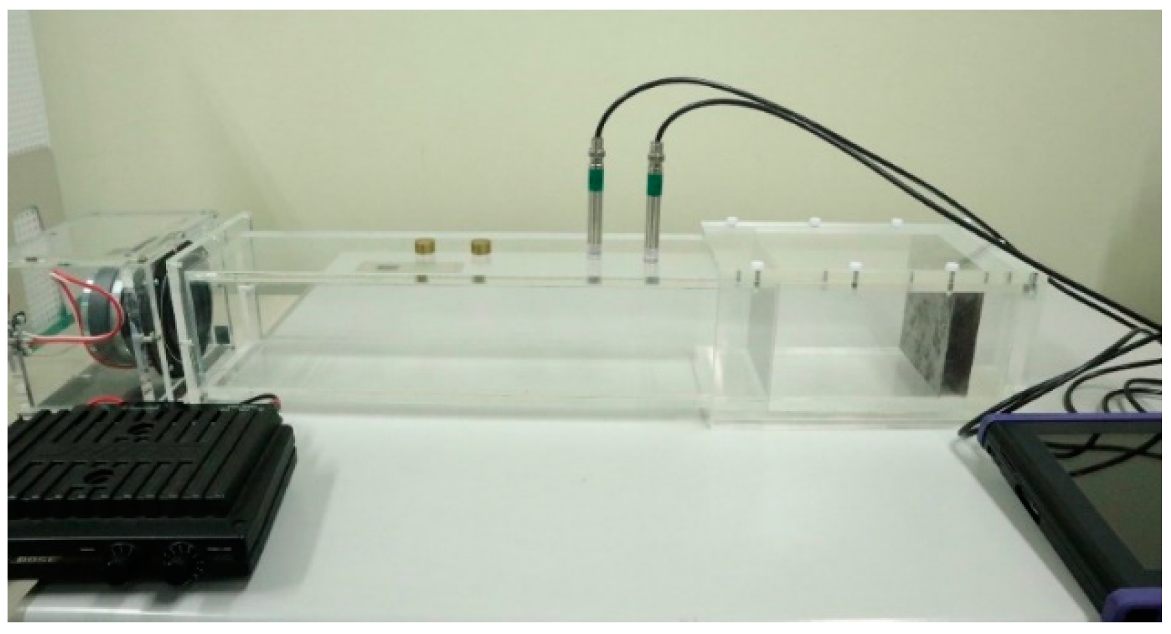
3.1.2. Experimental Setup
3.2. Prediction Error Indices and Classification According to the Error
- Group (1) has a relative error ferror of the frequency with the maximum sound absorption coefficient and a relative error αerror of the maximum sound absorption coefficient, both below 5%, and an RMS error of 0.05 or less.
- Group (3) has a relative error ferror of the frequency of the maximum sound absorption or a relative error αerror of the maximum value of sound absorption greater than 10% or an RMS error greater than 0.1.
- Specimens that do not fall into either group (1) or (3) were classified into group (2).
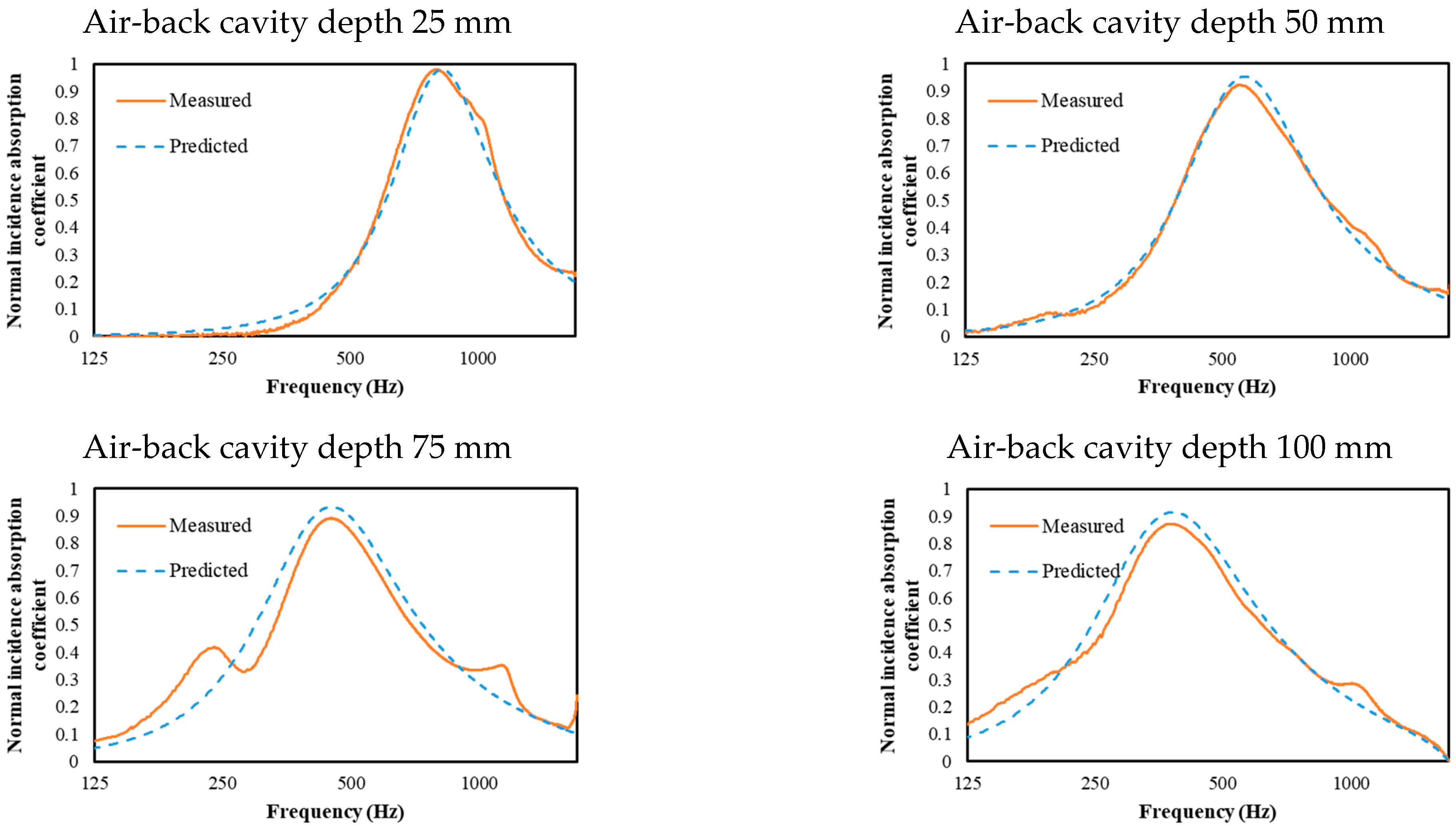
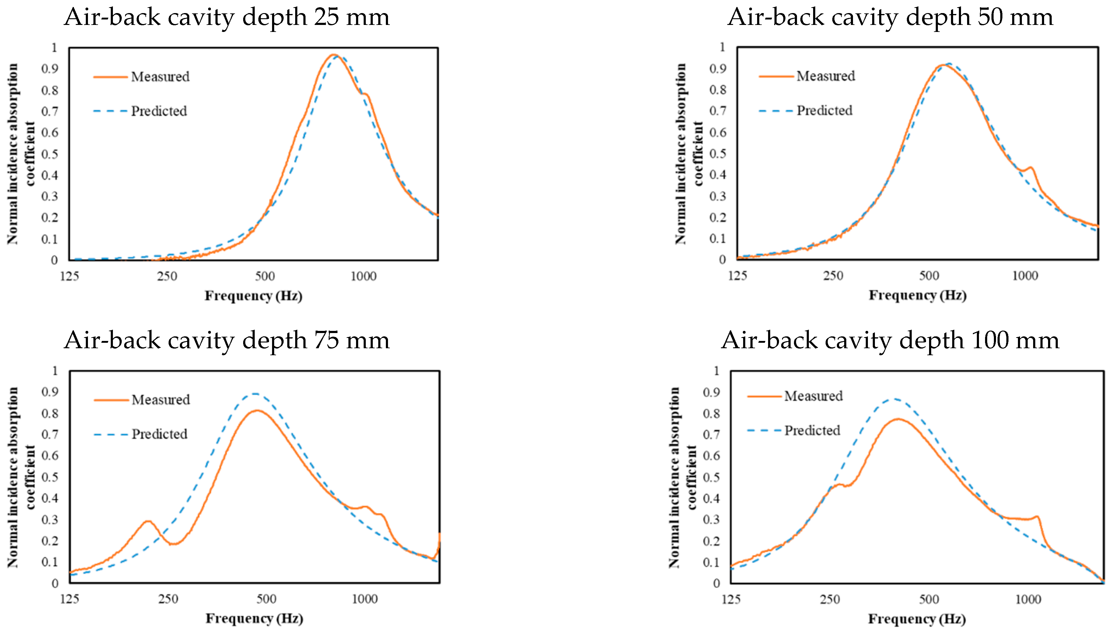
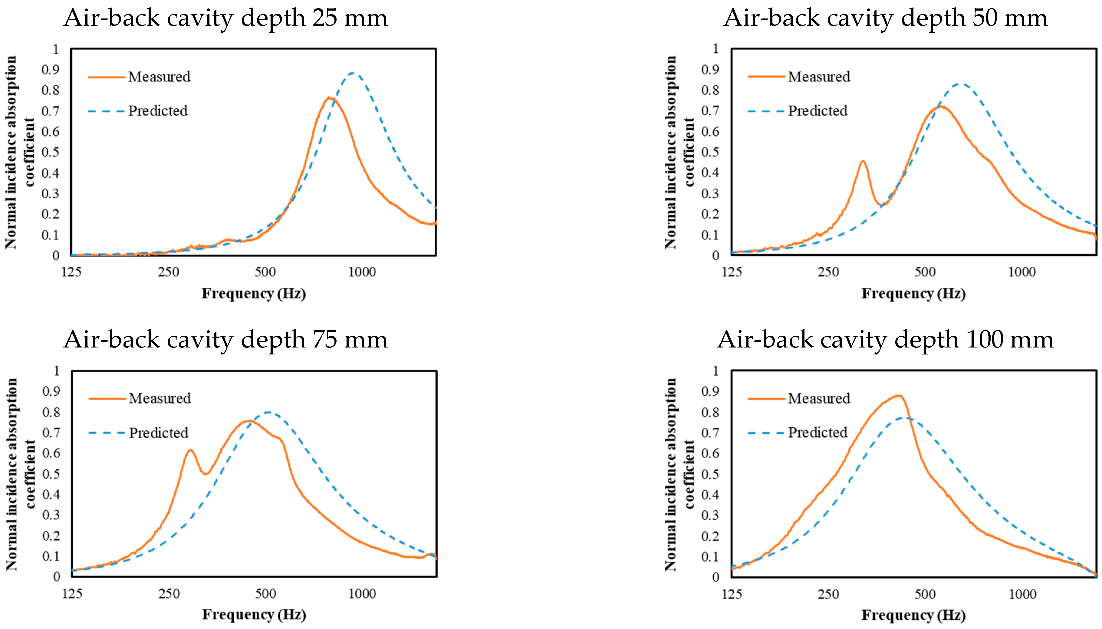
3.3. Results and Discussion
- Group (1).
- 2.
- Group (2).
- 3.
- Group (3).
- The number of hole types with different diameters is between 2 and 4;
- The holes are distributed over the entire surface of the specimen surface;
- The hole spacing is constant.
- The number of different hole types with different diameters is between 2 and 5;
- The holes are distributed over the entire surface of the specimen;
- The hole spacing is not always constant.
- The number of hole types with different diameters ranges from 1 to 5;
- The holes are distributed only in some parts of the specimen surface;
- The hole spacing is not constant.
4. Investigation by Prototyping Dotted-Art Heterogeneous MPPs
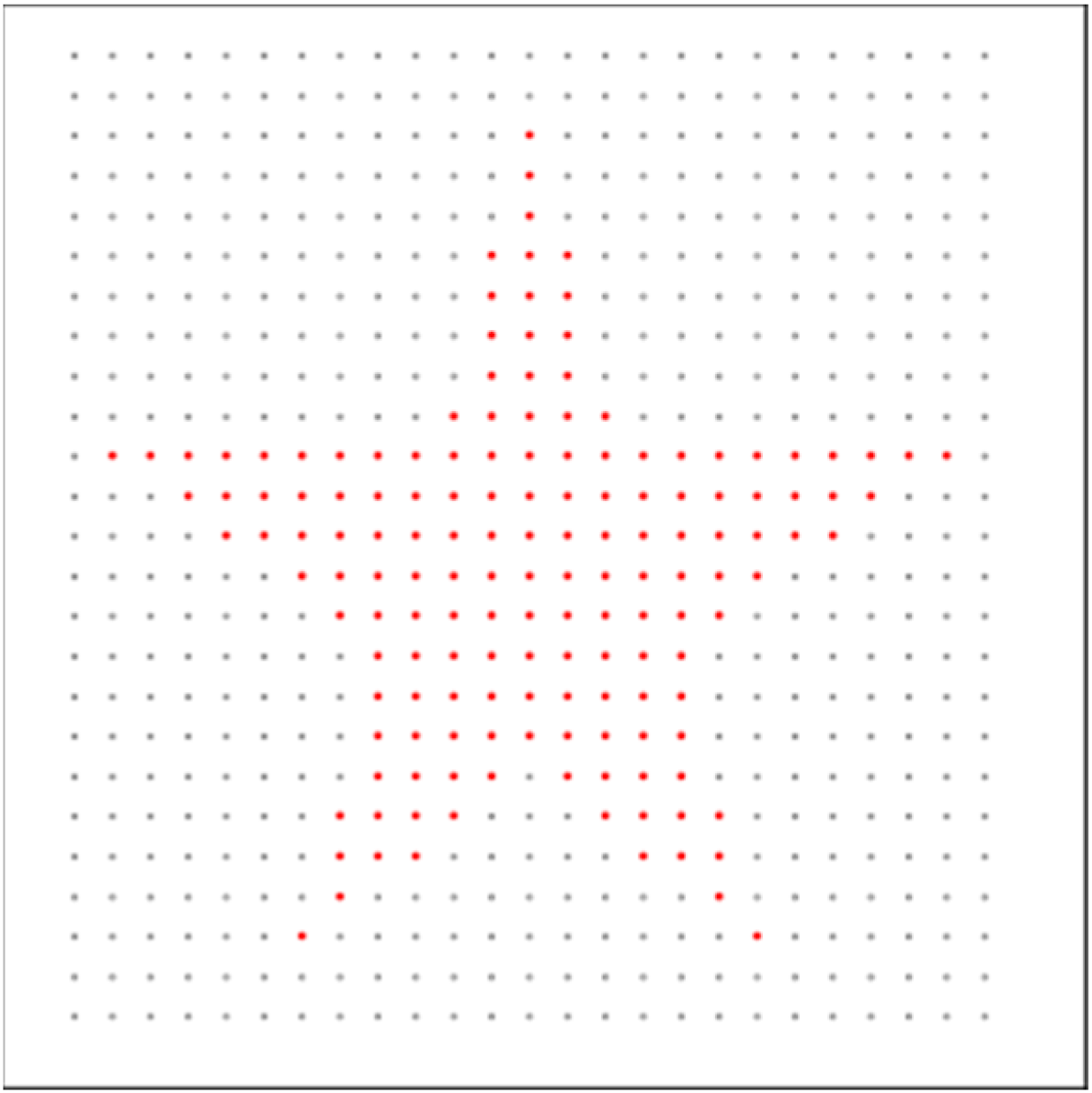
4.1. Design Concept of Dotted-Art Heterogeneous MPPs
- The holes are distributed over the entire surface of the absorber;
- The hole separation is constant over the entire surface of the absorber.
4.2. Preparation of the Specimens
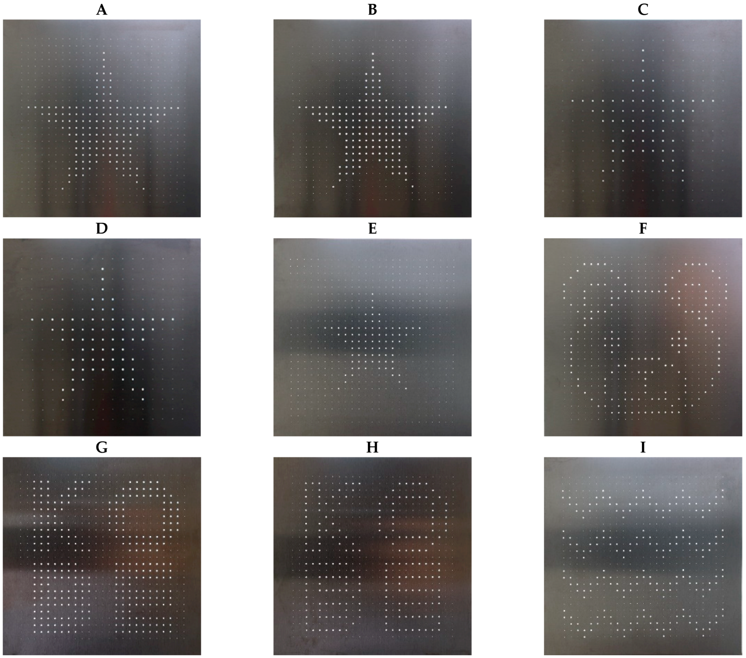
- Specimen A is made using 0.2 mm and 0.8 mm diameter holes in a star pattern and with a hole spacing of 4.0 mm.
- Specimen B is made using 0.2 mm and 1.0 mm diameter holes in a star pattern and with a hole spacing of 4.0 mm. The arrangement of the holes is identical to that of specimen A.
- Specimen C is a star pattern with 0.2 mm and 0.8 mm diameter holes, with a hole spacing of 6.0 mm. Although the hole spacing is different, the size of the star is almost the same as that in specimens A and B.
- Specimen D is made with 0.2 mm and 1.0 mm diameter holes and a hole spacing of 6.0 mm to express a star pattern. The arrangement of the holes is identical to that in specimen C.
- Specimen E is made using 0.2 mm and 0.8 mm diameter holes, with a hole spacing of 4.0 mm to produce a star pattern. The hole spacing and the type of holes used are the same as those in specimen A, but the size of the star pattern is smaller than that in specimen E.
- Specimen F is made using 0.2 mm and 0.8 mm diameter holes, with a hole spacing of 4.0 mm and expressing the pattern of a bear face.
- Specimen G is made of 0.2 mm and 0.8 mm holes and a hole spacing of 4.0 mm, which illustrate the bold letters ‘KOBE’.
- Specimen H is the outer frame of the bold letters ‘KOBE’, with holes of 0.2 mm and 0.8 mm in diameter and a hole spacing of 4.0 mm.
- Specimen I is a zigzag pattern, with holes of 0.2 mm and 0.8 mm in diameter and a hole spacing of 4.0 mm.
4.3. Method of Investigating Predictability
4.3.1. Experiment
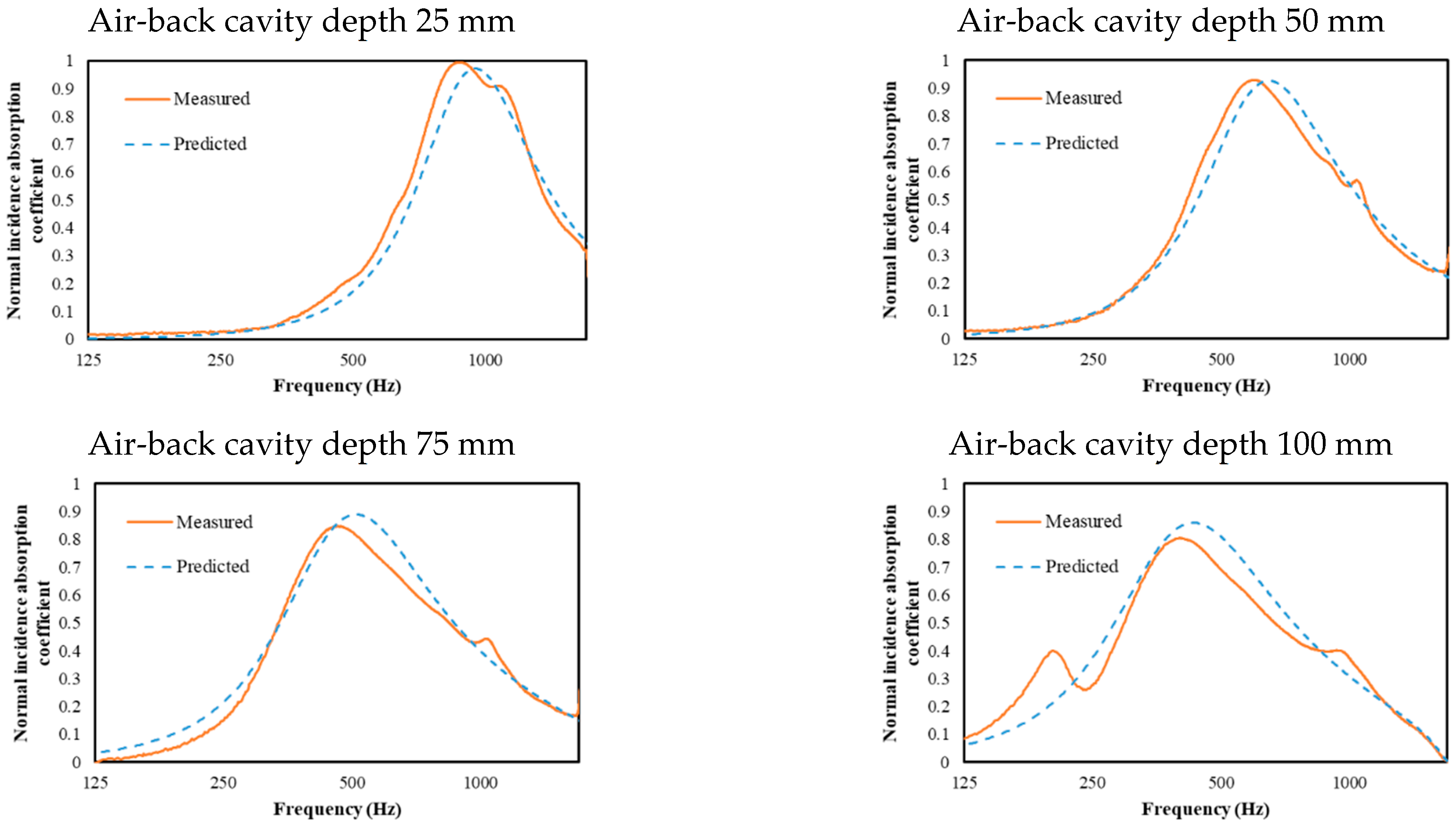
4.3.2. Results and Discussion
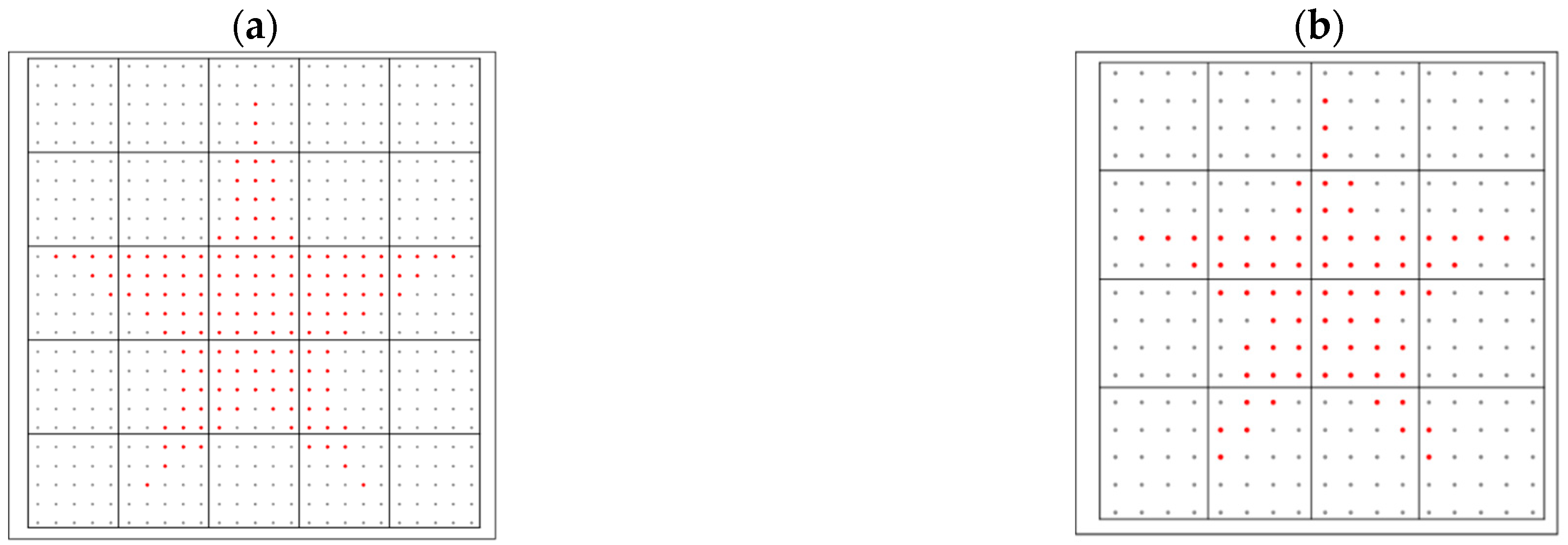
4.4. Effect of Hole Distribution on Prediction Accuracy
4.5. Effect of the Absence of Holes in the Background on Prediction Accuracy
5. Conclusions
- The SIM can predict the sound absorption characteristics of heterogeneous MPPs that satisfy the following two conditions: (1) the holes are distributed over the entire surface of the specimen, and (2) the hole spacing is constant.
- The condition of constant hole spacing is not essential for the application of the SIM, but it is considered to be a condition that enables a more reliable prediction.
- Heterogeneous MPPs with holes that are distributed in only a limited part of the specimen surface are likely to be outside the scope of the application of the SIM.
- When using the SIM to predict the sound absorption properties of heterogeneous MPPs, a number of different hole sizes is unlikely to influence prediction accuracy.
- The prediction accuracy for the specimens of dotted-art heterogeneous MPPs, designed according to the concept described above, tends to be good. This is because holes of the same diameter are unbiasedly distributed over the surface; i.e., the distribution of holes of the same diameter is less biased. Therefore, for the design of a dotted-art heterogeneous MPP, the distribution of holes of the same diameter should be as unbiased as possible.
- For dotted-art heterogeneous MPPs with a combination of two types of holes with different diameters: If the smaller holes in the background area are removed and only one type of hole is used in the patterned area of the heterogeneous MPP, the SIM is still applicable to the specimens (without smaller holes); however, prediction accuracy decreases. Therefore, a dotted-art heterogeneous MPP with two types of holes is better in terms of prediction accuracy.
Author Contributions
Funding
Data Availability Statement
Acknowledgments
Conflicts of Interest
Appendix A. Outline of Guo’s Theory
References
- Maa, D.-Y. Theory and design of microperforated panel sound-absorbing constructions. Sci. Sin. 1975, 17, 55–71. [Google Scholar]
- Sakagami, K.; Okuzono, T. Some considerations on the use of space sound absorbers with next-generation materials reflecting COVID situations in Japan: Additional sound absorption for post-pandemic challenges in indoor acoustic environments. UCL Open Environ. 2020, 1, 9. [Google Scholar] [CrossRef]
- Kang, J.; Fichs, H.V. Predicting absorption of open weave textiles and micro-perforated membranes backed by an air space. J. Sound Vib. 1999, 220, 905–920. [Google Scholar] [CrossRef]
- Fuchs, H.V.; Zha, X.; Zhou, X.; Drotleff, H. Creating low-noise environments in communication rooms. Appl. Acoust. 2001, 62, 1375–1396. [Google Scholar] [CrossRef]
- Zha, X.; Fuchs, H.V.; Drotleff, H. Improving the acoustic working conditions for musicians in small spaces. Appl. Acoust. 2002, 63, 203–221. [Google Scholar] [CrossRef]
- Kang, J.; Brocklesby, M.W. Feasibility of applying micro-perforated absorbers in acoustic window systems. Appl. Acoust. 2005, 66, 669–689. [Google Scholar] [CrossRef]
- Asdrubali, F.; Pispola, G. Properties of transparent sound-absorbing panels for use in noise barriers. J. Acoust. Soc. Am. 2007, 121, 214–221. [Google Scholar] [CrossRef]
- Herrin, D.; Liu, J.; Seybert, A. Properties and applications of microperforated panel. Sound Vib. 2011, 45, 6–9. [Google Scholar]
- Herrin, D. A guide to the applications of microperforated panel absorbers. Sound Vib. 2017, 51, 12–18. [Google Scholar]
- Adams, T. Sound Materials: A Compendium of Sound Absorbing Materials for Architecture and Design; Frame Pub: Amsterdam, The Netherland, 2017; pp. 214–231. [Google Scholar]
- Lee, H.P.; Kumar, S.; Aow, J.W. Proof-of-concept design for MPP acoustic absorbers with element of art. Designs 2021, 5, 72. [Google Scholar] [CrossRef]
- Maa, D.-Y. Microperforated-panel wideband absorbers. Noise Control Eng. J. 1987, 29, 77–84. [Google Scholar] [CrossRef]
- Maa, D.-Y. Potential of microperforated panel absorber. J. Acoust. Soc. Am. 1998, 104, 2861–2866. [Google Scholar] [CrossRef]
- Kusaka, M.; Sakagami, K.; Okuzono, T. A basic study on the absorption properties and their prediction of heterogeneous micro-perforated panels; A case study of micro-perforated poanels with heterogeneous hole size and perforation ratio. Acoustics 2021, 3, 473–484. [Google Scholar] [CrossRef]
- Sakagami, K.; Nagayama, Y.; Morimoto, M.; Yairi, M. Pilot study on wideband sound absorber obtained by combination of two different microperforated panel (MPP) absorbers. Acoust. Sci. Technol. 2009, 30, 154–156. [Google Scholar] [CrossRef] [Green Version]
- Yairi, M.; Sakagami, K.; Takebayashi, K.; Morimoto, M. Excess sound absorption at normal incidence by two microperforated panel absorbers with different impedance. Acoust. Sci. Technol. 2011, 32, 194–200. [Google Scholar] [CrossRef] [Green Version]
- Mosa, A.I.; Putra, A.; Ramlan, R.; Esraa, A. Wideband sound absorption of a double-layer microperforated panel with inhomogeneous perforation. Appl. Acoust. 2020, 161, 107167. [Google Scholar] [CrossRef]
- Pan, L.; Martellotta, F. A parametric study of the acoustic performance of resonant absorbers made of micro-perforated membranes and perforated panels. Appl. Sci. 2020, 10, 1581. [Google Scholar] [CrossRef] [Green Version]
- Sakagami, K.; Kusaka, M.; Okuzono, T.; Nakanishi, S. The effect of deviation due to the manufacturing accuracy in the parameters of an MPP on its acoustic properties; Trial production of MPPs of different hole shapes using 3D printing. Acoustics 2020, 2, 605–616. [Google Scholar] [CrossRef]
- Carbajo, J.; Ramis, I.; Godinho, L.; Amado-Mendes, P. Assessment of methods to study the acoustic properties of heterogeneous perforated panel absorbers. Appl. Acoust. 2018, 133, 1–7. [Google Scholar] [CrossRef]
- Guo, Y.; Allam, S.; Abon, M. Micro-Perforated Plates for Vehicle Applications. In Proceedings of the Inter-Noise 2008, Shanghai, China, 26–29 October 2008. [Google Scholar]
- Bolton, J.S.; Kim, N. Use of CFD to calculate the dynamic resistive end correction for microperforated materials with tapered holes. Acoust. Aust. 2010, 38, 134–144. [Google Scholar]
- Herdtle, T.; Bolton, J.S.; Kim, N.; Alexander, J.H.; Gardes, R.W. Transfer impedance of microperforated materials with tapered holes. J. Acoust. Soc. Am. 2013, 134, 4752–4762. [Google Scholar] [CrossRef] [PubMed] [Green Version]
- Okuzono, T.; Nitta, T.; Sakagami, K. Note on microperforated panel model using equivalent-fluid-based absorption elements. Acoust. Sci. Technol. 2019, 40, 221–224. [Google Scholar] [CrossRef] [Green Version]
- JIS A 1405-2: 2007; Acoustics—Determination of Sound Absorption Coefficient and Impedance in Impedance Tubes—Part 2: Transfer-Function Method. JIS: Tokyo, Japan, 2007.
- ISO 10534-2:1998; Acoustics—Determination of Sound Absorption Coefficient and Impedance in Impedance Tubes—Part 2: Transfer-Function Method. ISO: Geneva, Switzerland, 1998.


| Specimen | Diameter (mm) and (Number of Holes) | Hole Separation (mm) | Average Perforation Ratio (%) | Thickness of the Plate (mm) |
|---|---|---|---|---|
| 1 | 0.3 (60), 0.5 (60), 0.7 (60), 0.9 (45) | 6.0 | 0.6774 | 0.5 |
| 2 | 0.3 (120), 0.9 (105) | 6.0 | 0.7528 | 0.5 |
| 3 | 0.3 (120), 0.9 (105) | 6.0 | 0.7528 | 0.5 |
| 4 | 0.3 (4), 0.5 (12), 0.7 (20), 0.9 (28), 1.1 (36) | 10.0 | 0.6236 | 0.5 |
| 5 | 0.3 (113), 0.9 (112) | 6.0 | 0.7924 | 0.5 |
| 6 | 0.3 (60), 0.5 (60), 0.7 (60), 0.9 (45) | 6.0 | 0.6774 | 0.5 |
| 7 | 0.3 (10), 0.5 (30), 0.7 (50), 0.9 (70), 1.1 (90) | 3.142 on all circumferences | 1.559 | 0.5 |
| 8 | 0.5 (45), 0.7 (45), 0.9 (45), 1.1 (60) | On all the circumferences from inside to outside: 1.117, 1.518, 2.225, 2.985 | 1.118 | 1.0 |
| 9 | 1.0 (48) | 5.0 | 0.3770 | 0.5 |
| 10 | 1.0 (60) | 3.142 | 0.4712 | 0.5 |
| 11 | 1.0 (100) | 2.513 | 0.7854 | 0.5 |
| 12 | 0.5 (121) | 5.0 | 0.2376 | 0.5 |
| Specimen | ferror (%) | αerror (%) | RMS Error |
|---|---|---|---|
| 1 | 1.540 | 3.223 | 0.04191 |
| 2 | 3.675 | 2.632 | 0.03966 |
| Specimen | ferror (%) | αerror (%) | RMS Error |
|---|---|---|---|
| 3 | 3.591 | 5.730 | 0.04853 |
| 4 | 2.704 | 4.656 | 0.05104 |
| 5 | 1.038 | 5.588 | 0.04313 |
| 6 | 2.242 | 5.036 | 0.03980 |
| 7 | 7.938 | 3.657 | 0.04662 |
| Specimen | ferror (%) | αerror (%) | RMS Error |
|---|---|---|---|
| 8 | 13.69 | 11.95 | 0.1424 |
| 9 | 4.467 | 13.39 | 0.08091 |
| 10 | 2.310 | 13.24 | 0.08296 |
| 11 | 9.604 | 14.29 | 0.09839 |
| 12 | 11.18 | 8.632 | 0.09974 |
| Specimen | Diameter (mm) and (Number of Holes) | Hole Separation (mm) | Average Perforation Ratio (%) | Thickness of the Plate (mm) |
|---|---|---|---|---|
| A | 0.2 (469), 0.8 (156) | 4.0 | 0.9315 | 0.5 |
| B | 0.2 (469), 1.0 (156) | 4.0 | 1.373 | 0.5 |
| C | 0.2 (216), 0.8 (73) | 6.0 | 0.4348 | 0.5 |
| D | 0.2 (216), 1.0 (73) | 6.0 | 0.6412 | 0.5 |
| E | 0.2 (546), 0.8 (79) | 4.0 | 0.5686 | 0.5 |
| F | 0.2 (470), 0.8 (150) | 4.0 | 0.6774 | 0.5 |
| G | 0.2 (318), 0.8 (307) | 4.0 | 1.643 | 0.5 |
| H | 0.2 (417), 0.8 (208) | 4.0 | 1.177 | 0.5 |
| I | 0.2 (425), 0.8 (200) | 4.0 | 1.139 | 0.5 |
| Specimen | ferror (%) | αerror (%) | RMS Error |
|---|---|---|---|
| A | 8.598 | 3.640 | 0.05230 |
| B | 7.356 | 3.001 | 0.04935 |
| C | 6.846 | 3.147 | 0.08007 |
| D | 1.100 | 8.184 | 0.06381 |
| E | 3.205 | 2.295 | 0.04886 |
| F | 0.8354 | 5.409 | 0.03031 |
| G | 2.718 | 4.792 | 0.03080 |
| H | 1.842 | 4.409 | 0.02988 |
| I | 1.631 | 2.206 | 0.02379 |
| Specimen A | Specimen B | Specimen C | |||
|---|---|---|---|---|---|
| SD | 33.45 | SD | 33.45 | SD | 30.72 |
| ferror (%) | 8.598 | ferror (%) | 7.356 | ferror (%) | 6.846 |
| αerror (%) | 3.640 | αerror (%) | 3.001 | αerror (%) | 3.147 |
| RMS error | 0.05230 | RMS error | 0.04935 | RMS error | 0.08007 |
| Specimen D | Specimen E | Specimen D | |||
| SD | 30.72 | SD | 23.96 | SD | 11.81 |
| ferror (%) | 1.100 | ferror (%) | 3.205 | ferror (%) | 0.8354 |
| αerror (%) | 8.184 | αerror (%) | 2.295 | αerror (%) | 5.409 |
| RMS error | 0.06381 | RMS error | 0.04886 | RMS error | 0.03031 |
| Specimen G | Specimen H | Specimen I | |||
| SD | 19.02 | SD | 10.16 | SD | 5.426 |
| ferror (%) | 2.718 | ferror (%) | 1.842 | ferror (%) | 1.631 |
| αerror (%) | 4.792 | αerror (%) | 4.409 | αerror (%) | 2.206 |
| RMS error | 0.03080 | RMS error | 0.02988 | RMS error | 0.02379 |
| ferror (%) | αerror (%) | RMS Error | ||||
|---|---|---|---|---|---|---|
| With | Without | With | Without | With | Without | |
| Specimens A, A’ | 8.598 | 9.361 | 3.640 | 8.239 | 0.05230 | 0.07576 |
| Specimens B, B’ | 7.356 | 8.016 | 3.001 | 9.256 | 0.04935 | 0.08741 |
| Specimens C, C’ | 6.846 | 6.413 | 3.147 | 8.076 | 0.08007 | 0.08845 |
| Specimens D, D’ | 1.100 | 1.478 | 8.184 | 12.66 | 0.06381 | 0.07217 |
| Specimens E, E’ | 3.205 | 3.675 | 2.295 | 16.06 | 0.04886 | 0.1076 |
| Specimens F, F’ | 0.8354 | 1.112 | 5.409 | 7.030 | 0.03031 | 0.05351 |
| Specimens G, G’ | 2.718 | 2.236 | 4.792 | 5.564 | 0.03080 | 0.04364 |
| Specimens H, H’ | 1.611 | 4.373 | 4.640 | 8.494 | 0.02988 | 0.04858 |
| Specimens I, I’ | 1.631 | 2.506 | 2.206 | 7.442 | 0.02379 | 0.03993 |
Publisher’s Note: MDPI stays neutral with regard to jurisdictional claims in published maps and institutional affiliations. |
© 2022 by the authors. Licensee MDPI, Basel, Switzerland. This article is an open access article distributed under the terms and conditions of the Creative Commons Attribution (CC BY) license (https://creativecommons.org/licenses/by/4.0/).
Share and Cite
Sakagami, K.; Kusaka, M.; Okuzono, T. A Basic Study on the Design of Dotted-Art Heterogeneous MPP Sound Absorbers. Acoustics 2022, 4, 588-608. https://doi.org/10.3390/acoustics4030037
Sakagami K, Kusaka M, Okuzono T. A Basic Study on the Design of Dotted-Art Heterogeneous MPP Sound Absorbers. Acoustics. 2022; 4(3):588-608. https://doi.org/10.3390/acoustics4030037
Chicago/Turabian StyleSakagami, Kimihiro, Midori Kusaka, and Takeshi Okuzono. 2022. "A Basic Study on the Design of Dotted-Art Heterogeneous MPP Sound Absorbers" Acoustics 4, no. 3: 588-608. https://doi.org/10.3390/acoustics4030037