
Underwater Target Localization Using Opportunistic Ship Noise Recorded on a Compact Hydrophone Array

 , ,
, ,
Abstract
: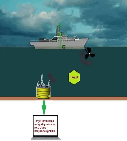
1. Introduction
2. Theoretical Background
2.1. The Lloyd–Mirror Pattern (LMP)
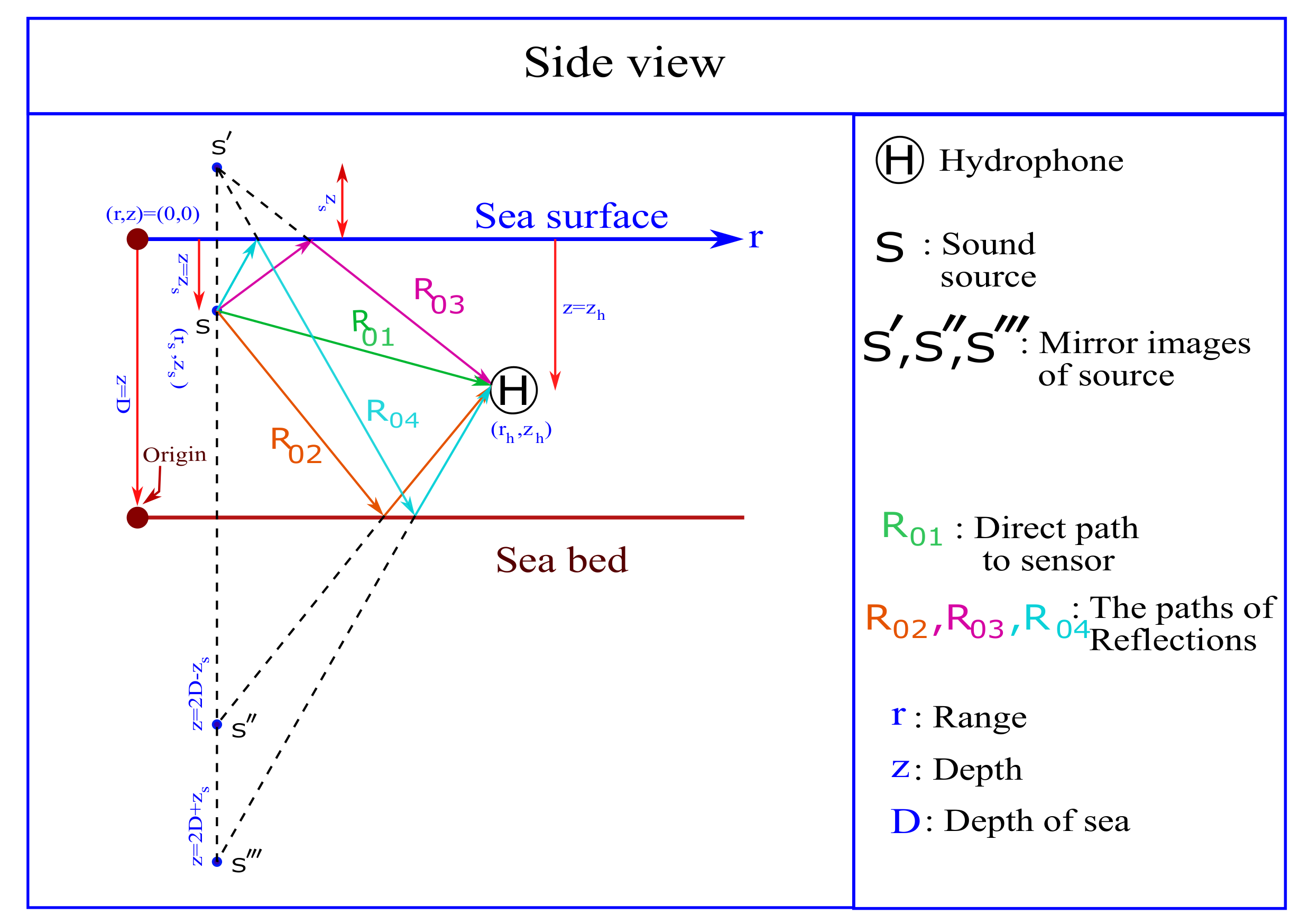
2.2. The Image Model
2.3. The Normal-Mode Model in an Isovelocity Environment
- (1)
- A pressure release at the surface ();
- (2)
- A perfectly rigid bottom with lossless reflection at the sea bottom, i.e., when . Note that, on a first order approximation, this assumption is valid for the test conditions in this work since the bottom is rocky [9].
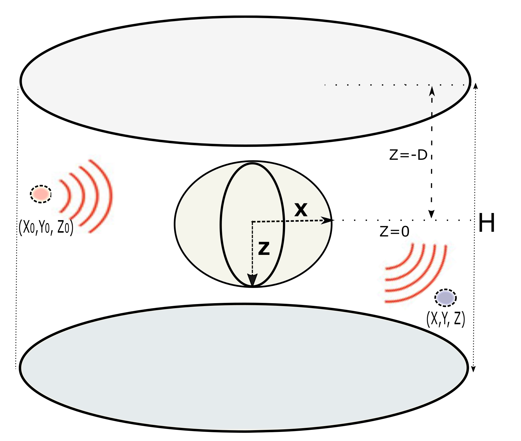
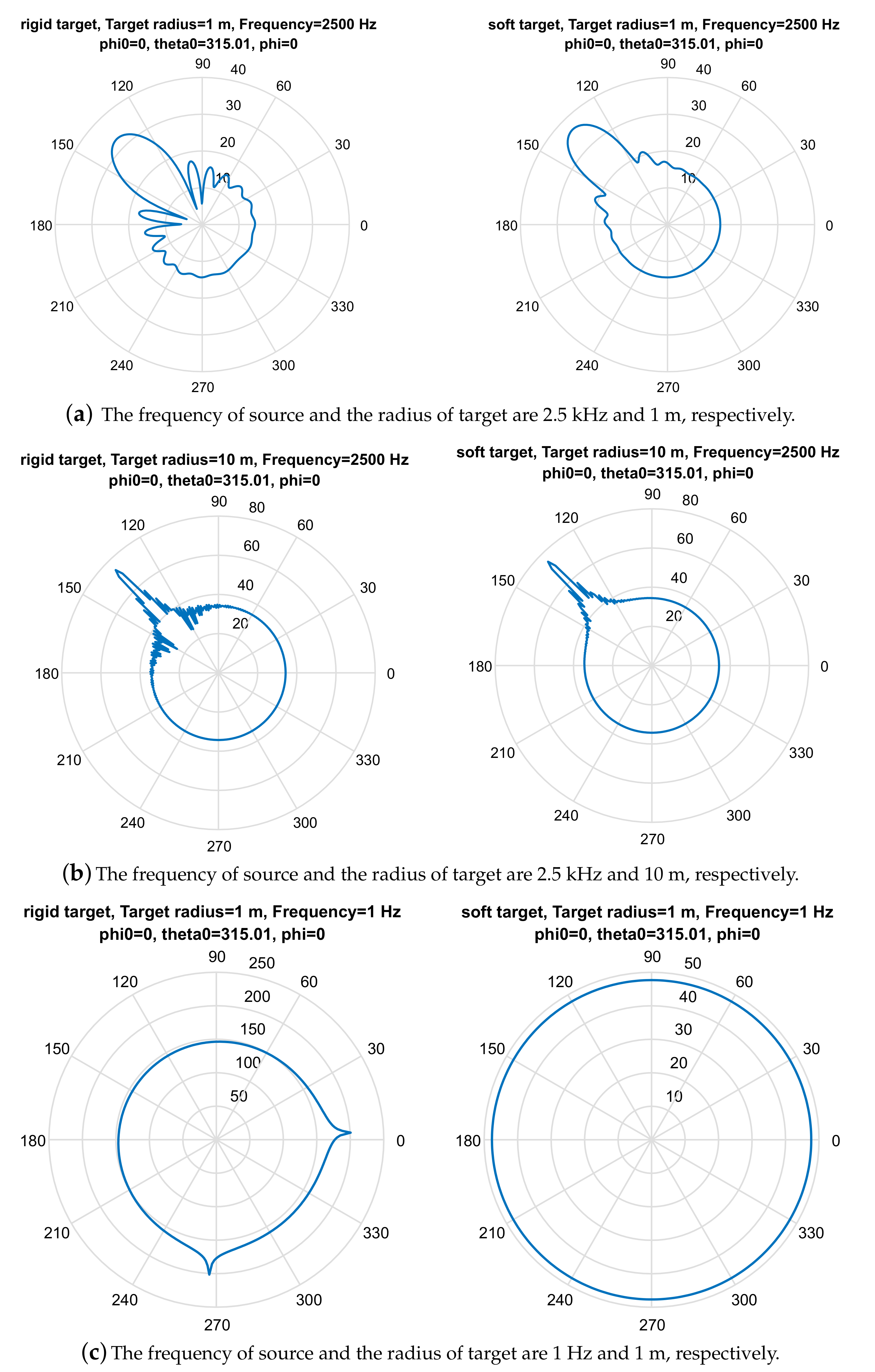
2.4. Scattering Field from Targets in a Waveguide
3. Methods and Material
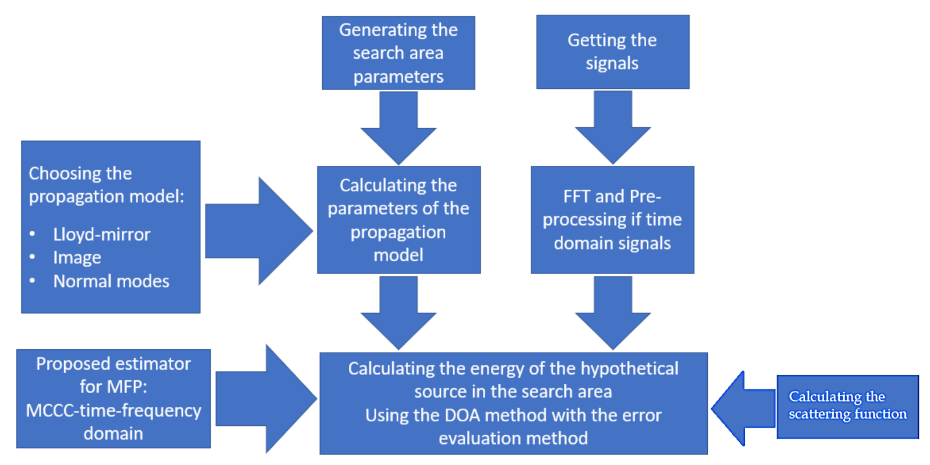
3.1. Proposed Localization Algorithm for MFP
3.2. Experimental Setup and Data Collection
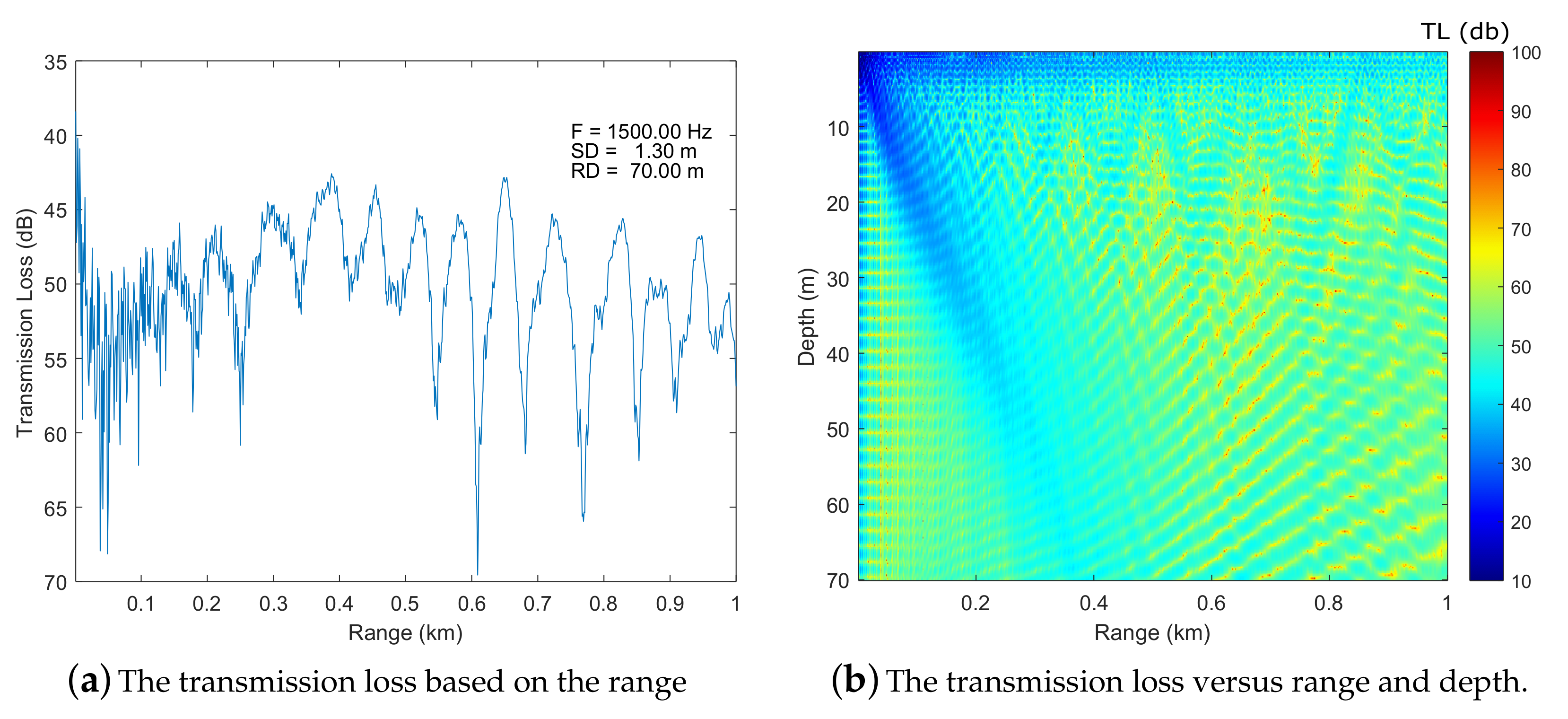
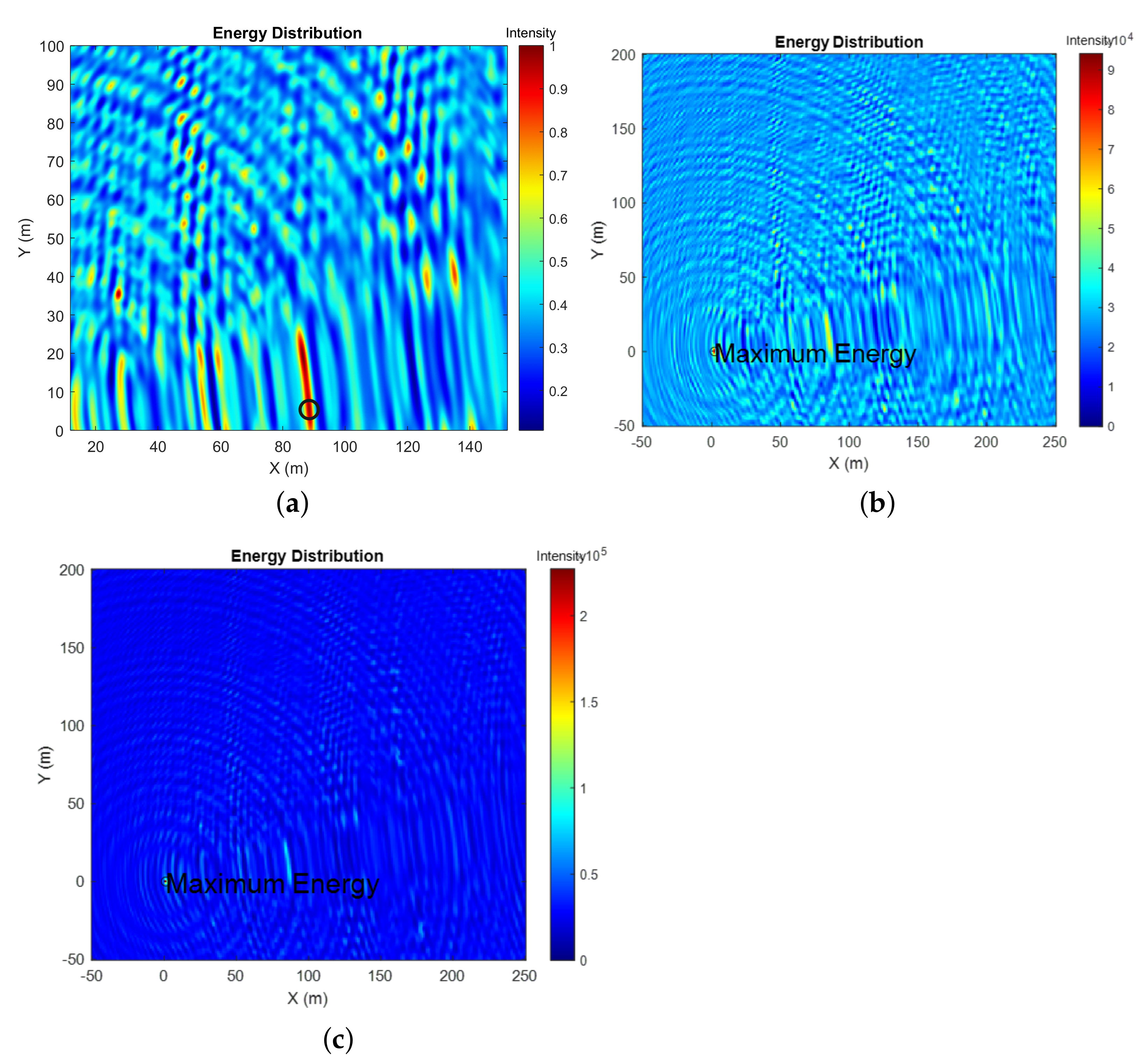
4. Simulation Results
Simulation Using the Synthetic Data
5. Conclusions
Author Contributions
Funding
Institutional Review Board Statement
Informed Consent Statement
Data Availability Statement
Acknowledgments
Conflicts of Interest
References
- Verlinden, C.M. Acoustic Sources of Opportunity in the Marine Environment-Applied to Source Localization and Ocean Sensing. Ph.D. Thesis, University of California, San Diego, CA, USA, 2017. [Google Scholar]
- Park, C.; Seong, W.; Gerstoft, P. Geoacoustic inversion in time domain using ship of opportunity noise recorded on a horizontal towed array. J. Acoust. Soc. Am. 2005, 117, 1933–1941. [Google Scholar] [CrossRef] [PubMed]
- Tollefsen, D.; Dosso, S.E. Bayesian geoacoustic inversion of ship noise on a horizontal array. J. Acoust. Soc. Am. 2008, 145, 788–795. [Google Scholar] [CrossRef] [PubMed]
- Tollefsen, D.; Dosso, S.E.; Knobles, D.P. Ship-of-opportunity noise inversions for geoacoustic profiles of a layered mud-sand seabed. IEEE J. Ocean. Eng. 2008, 45, 189–200. [Google Scholar] [CrossRef]
- Knobles, D.P. Maximum entropy inference of seabed attenuation parameters using ship radiated broadband noise. J. Acoust. Soc. Am. 2015, 138, 3563–3575. [Google Scholar] [CrossRef] [PubMed] [Green Version]
- Mirzaei Hotkani, M.; Seyedin, S.A.; Bousquet, J.-F. Estimation of the Bistatic Echolocation from Underwater Target Using Ship Noise based on Normal-Mode Model, Signal Processing and Renewable Energy. Signal Process. Renew. Energy SPRE 2020, 5, 1–14. [Google Scholar]
- McKenna, M.F.; Ross, D.; Wiggins, S.M.; Hildebrand, J.A. Underwater radiated noise from modern commercial ships. J. Acoust. Soc. Am. 2012, 131, 92–103. [Google Scholar] [CrossRef] [PubMed] [Green Version]
- Viitanen, V.M.; Hynninen, A.; Sipilä, T.; Siikonen, T. DDES of Wetted and Cavitating Marine Propeller for CHA Underwater Noise Assessment. J. Mar. Sci. Eng. 2018, 6, 56. [Google Scholar] [CrossRef] [Green Version]
- Jensen, F.B.; Kuperman, W.A.; Porter, M.B.; Schmidt, H. Computational Ocean Acoustics, 2nd ed.; Springer Science and Business Media: Berlin/Heidelberg, Germany, 2011. [Google Scholar]
- Zimmer, W.M.X. Principles of Underwater Sound in Passive Acoustic Monitoring of Cetaceans, 3rd ed.; Cambridge University Press: Cambridge, UK, 2011. [Google Scholar]
- Hovem, J.M. Underwater acoustics: Propagation, devices and systems. J. Electroceram. 2007, 19, 339–347. [Google Scholar] [CrossRef]
- Cobos, M.; Antonacci, F.; Alexandridis, A.; Mouchtaris, A.; Lee, B. A survey of sound source localization methods in wireless acoustic sensor networks. Wirel. Commun. Mob. Comput. 2017, 2017, 3956282. [Google Scholar] [CrossRef]
- Wu, P.; Su, S.; Zuo, Z.; Guo, X.; Sun, B.; Wen, X. Time Difference of Arrival (TDoA) Localization Combining Weighted Least Squares and Firefly Algorithm. Sensors 2019, 19, 2554. [Google Scholar] [CrossRef] [PubMed] [Green Version]
- Wang, L.; Yang, Y.; Liu, X. A distributed subband valley fusion (DSVF) method for low frequency broadband target localization. J. Acoust. Soc. Am. 2018, 143, 2269–2278. [Google Scholar] [CrossRef] [PubMed]
- Wang, L.; Yang, Y.; Liu, X. A cluster-based direct source localization approach for large-aperture horizontal line arrays. J. Acoust. Soc. Am. 2020, 147, EL50–EL54. [Google Scholar] [CrossRef] [PubMed]
- Lo, K.W. A matched-field processing approach to ranging surface vessels using a single hydrophone and measured replica fields. J. Acoust. Soc. Am. 2021, 149, 1466–1474. [Google Scholar] [CrossRef] [PubMed]
- Mesmoudi, A.; Feham, M.; Labraoui, N. Wireless sensor networks localization algorithms: A comprehensive survey. Int. J. Comput. Netw. Commun. 2013, 45–64. [Google Scholar] [CrossRef]
- Michalopoulou, Z.-H.; Gerstoft, P.; Caviedes-Nozal, D. Matched field source localization with Gaussian processes. JASA Express Lett. 2021, 1, 064801. [Google Scholar] [CrossRef]
- Tran, P.N.; Trinh, K.D. Adaptive Matched Field Processing for Source Localization Using Improved Diagonal Loading Algorithm. Acoust. Aust 2017, 45, 325–330. [Google Scholar] [CrossRef]
- Evans, R.B.; Di, X.; Gilbert, K.E. A Legendre-Galerkin spectral method for constructing atmospheric acoustic normal modes. J. Acoust. Soc. Am. 2018, 143, 3595–3601. [Google Scholar] [CrossRef] [PubMed]
- Zhang, T.; Yang, T.C.; Xu, W. Channel distortion on target scattering amplitude in shallow water. J. Acoust. Soc. Am. 2019, 146, EL470–EL476. [Google Scholar] [CrossRef] [PubMed]
- Ingenito, F. Scattering from an object in a stratified medium. J. Acoust. Soc. Am. 1987, 82, 2051–2059. [Google Scholar] [CrossRef]
- Benesty, J.; Chen, J.; Huang, Y. Microphone Array Signal Processing; Springer: Berlin/Heidelberg, Germany, 2018. [Google Scholar]


| Parameters | Values |
|---|---|
| The sound speed | m/s |
| Depth of water | m |
| Depth of source | m |
| Depth of Receiver | m |
| The average source frequency | Hz |
| Latitude | Longitude | Depth | |
|---|---|---|---|
| Target | 44.480366 | −63.51195 | 25 m |
| Hydrophone array | 44.4803 | −63.513115 | 70 m |
| Parameters | Values |
|---|---|
| Target diameter | 1.6 m |
| The actual range of the target from the array | 93 m |
| Depth of the target position from the ocean surface | 25 m |
| Type of the target | Rigid |
| Depth of ocean | 71.625 m |
| Maximum number of polynomials in Legendre function | 15 |
| Number of normal modes | 80 |
| Number of paths used in the image model | 4 paths |
| Sound speed in ocean | 1490 m/s |
| Sound speed on seabed | 1600 m/s |
| Desired frequency range | 500–2000 Hz |
| Density of water |
| Propagation Model | Estimated Target Location (x, y, z) | The Horizontal Range Relative Error | The Radial Range Relative Error |
|---|---|---|---|
| Normal-mode | (89 m, 29 m, 24.8 m) | 0.68% | 0.63% |
| Image | (91 m, 9 m, 24.8 m) | 1.64% | 1.24% |
| Lloyd-mirror | (116 m, 5 m, 24.8 m) | 24.88% | 20.62% |
| Propagation Model | Estimated Target Location (x, y, z) | The Horizontal Range Relative Error | The Radial Range Relative Error |
|---|---|---|---|
| Normal-mode | (88 m, 4 m, 24.2 m) | 5.2786% | 3.8774% |
| Image | (0 m, 0 m, 24.2 m) | 100% | 55.65% |
| Lloyd-mirror | (0 m, 0 m, 24.2 m) | 100% | 55.65% |
| Normal-mode | (85 m, 19 m, 24.2 m) | 6.3467% | 4.7295% |
| Image | (91 m, 6 m, 24.2 m) | 1.90% | 1.19% |
| Lloyd-mirror | (91 m, 6 m, 24.2 m) | 1.90% | 1.19% |
Publisher’s Note: MDPI stays neutral with regard to jurisdictional claims in published maps and institutional affiliations. |
© 2021 by the authors. Licensee MDPI, Basel, Switzerland. This article is an open access article distributed under the terms and conditions of the Creative Commons Attribution (CC BY) license (https://creativecommons.org/licenses/by/4.0/).
Share and Cite
Mirzaei Hotkani, M.; Bousquet, J.-F.; Seyedin, S.A.; Martin, B.; Malekshahi, E. Underwater Target Localization Using Opportunistic Ship Noise Recorded on a Compact Hydrophone Array. Acoustics 2021, 3, 611-629. https://doi.org/10.3390/acoustics3040039
Mirzaei Hotkani M, Bousquet J-F, Seyedin SA, Martin B, Malekshahi E. Underwater Target Localization Using Opportunistic Ship Noise Recorded on a Compact Hydrophone Array. Acoustics. 2021; 3(4):611-629. https://doi.org/10.3390/acoustics3040039
Chicago/Turabian StyleMirzaei Hotkani, Mojgan, Jean-Francois Bousquet, Seyed Alireza Seyedin, Bruce Martin, and Ehsan Malekshahi. 2021. "Underwater Target Localization Using Opportunistic Ship Noise Recorded on a Compact Hydrophone Array" Acoustics 3, no. 4: 611-629. https://doi.org/10.3390/acoustics3040039