Data Mining Applied to the Electrochemical Noise Technique in the Time/Frequency Domain for Stress Corrosion Cracking Recognition

Abstract

In this paper, time/frequency domain data processing was proposed to analyse the EN signal recorded during stress corrosion cracking on precipitation-hardening martensitic stainless steel in a chloride environment. Continuous Wavelet Transform, albeit with some limitations, showed a suitable support in the discriminatory capacity among transient signals related to the different stress corrosion cracking mechanisms. In particular, the aim is to propose the analysis of electrochemical noise signals under stress corrosion cracking conditions in the time–frequency domain by using the Hilbert–Huang approach. The Hilbert–Huang Transform (performed by the Empirical Mode Decomposition approach) was finally proposed to carry out an identification of the corrosion mechanisms in comparison to conventional data processing methods. By using this approach, a detailed simultaneous decomposition of the original electrochemical noise data in the time and frequency domain was carried out. The method gave useful information about transitions among different corrosion mechanisms, allowing us to (i) identify a specific characteristic response for each corrosion damaging phenomenon induced by stress corrosion cracking, (ii) time each corrosion of the damaging phenomenon, and (iii) provide a topological description of the advancing SCC damaging stages. This characteristic evidences that the Hilbert–Huang Transform is a very powerful technique to potentially recognize and distinguish the different corrosion mechanisms occurring during stress corrosion cracking.

1. Introduction

Stress corrosion cracking (SCC) represents one of the most crucial corrosion processes that can result in early catastrophic failures of structural parts or system, significantly reducing its life cycle. As a result, the adoption of a non-intrusive in situ assessment technique looks to be an intriguing way for obtaining knowledge and determining definite parameters in SCC procedures. Furthermore, various attempts are being made in the scientific community to develop NDT methods for monitoring stressed parts subjected to corrosive environments [1,2,3,4].

Among the several electrochemical techniques, electrochemical noise (EN) could potentially be considered most suitable for the assessment of damage evolution during SCC. Because this technology relies on spontaneous current and potential fluctuations created by corrosion processes, one of its primary advantages is its non-invasiveness [5,6].

Electrochemical noise (EN) can be applied to monitor and identify, in situ, the corrosion processes of metallic materials [7], and additionally monitor and assess the type and rate of corrosion in different harmful environments [8]. It can also be used to monitor the durability of coated metals [6,9]. Furthermore, this technique can detect localized corrosion, which affects small areas of the metal surface, as well as uniform corrosion, which affects the whole surface [10].

Indeed, various research efforts have shown that by using EN measurements, it is feasible to identify and discriminate between distinct forms of localized corrosion. [10], such as pitting [11], crevice [12], uniform corrosion [13], and stress-corrosion cracking [14].

In particular, as a reference, but not limited to, in [11], the stable and metastable pitting corrosion behaviour, pit initiation and growth in SLM 316L SS, via wavelet and stochastic analysis of ECN signals, were assessed.

Furthermore, in [12], localised crevice corrosion was investigated. Given that the mechanistic evaluation of localized corrosion mechanisms, with regard to electrochemical variables influencing the corrosion phenomena, is a critical point of discrimination, a combination of electrochemical impedance spectroscopy (EIS) and electrochemical noise (EN) approach using the Hilbert analysis was advantageously used.

Similarly, excellent potential for analysis of uniform corrosion using EN has been highlighted in several research activities [13], for which the uniform corrosion rate has been quantified by combining statistical characteristics and frequency domain analysis.

Analogously, the EN technique can be effectively applied to a complex phenomenon, such as stress corrosion cracking for a valuable detection of damage phenomena in SCC endorsing environment [14].

In this concern, studies performed on stainless steel under various conditions [15,16] showed that on SCC tests, it may be feasible to quantify electrochemical current and voltage noise variations caused by the cyclical activation and propagation of cracks. In a lot of research activities [17,18,19], hydrogen embrittlement and the impact of the related evolved hydrogen bubbles on the EN transient was accurately investigated.

SCC can form by either continuous and discontinuous mechanisms, characterized by quite distinct EN features. The discontinuous crack growth phenomenon is able to generate some distinctive current transients, whereas the continuous crack growth approach might generate low noise levels [20]. Therefore, EN has a substantial advantage over other methods for understanding the mechanism of SSC.

Although, it is difficult to link the crack tip activity with the fracture propagation rate and the EN response data, as observed in [21], the technique verifies the estimation of stress-corrosion thresholds and, considering that EN signal increased with activity at the crack tip, can be used to analyse the influence factors have on cracking.

An EN signal could be analysed in the time domain (by means of visual analysis, statistical analysis, such as maxima and minima recognition, or identification of statistical moments and other statistical parameters) or in the frequency domain (by means of Fast Fourier Transform (FFT), Power Spectral Density (PSD), Hilbert Transform (HT), Wavelet Transform (WT) and many other techniques).

To know beforehand whether a processed signal is stationary and linear is generally difficult. Thus, there is a risk that not all appropriate signal analysis methods could be used, therefore obtaining non-reliable results.

To limit this problem, the use of transforms such as FFT and PSD, which in fact require stationary and linear conditions, are applied for the limited signal time window, whose size is chosen to ensure the hypothesis of constant signal amplitude and linearity [22,23]. Therefore, the modified analysis becomes the so-called Short-term FT (STFT) [24,25,26], which shows critical issues on the choice of time window size, and, generally, provides a compromise between the assumption of stationariness and frequency resolution. Furthermore, typically acquired signals are a superposition of different signals from different sources (electrochemical dissolution, temperature drift, bubbles evolution...), each one with different intervals of stationary, so it is difficult to discriminate the correct values of each corrosion process.

Taking into account the aforementioned factors, traditional EN analysis approaches are insufficient to allow a clear discrimination among the different damage stages during the corrosion evolution in a component or system. Therefore, the use of a powerful time-dependent signal processing technique for data analysis should be evaluated.

The constant wavelet transform (CWT) was introduced to overcome the principal FFT theoretical limitation [27]; it furnishes a native energy/time/frequency representation, and it could be applied to the non-stationary signals due to its regional convolution mechanism. This method was successfully applied to the load variation analysis [24] and to the corrosion field [27]. However, it maintains a theoretical limitation on the applicability to non-linear signals, and, furthermore, there is an approximation related to the frequency/time resolution that should be taken into account.

A promising analysis method for non-stationary and non-linear signals of recorded EN data, which can be used to substitute or corroborate traditional time-dependent or frequency-dependent approaches, is the Hilbert–Huang Transform (HHT) [28]. The ability to analyse non-stationary and non-linear signals is the main advantage of HHT compared to ordinary signal analysis methods [29]. This relatively novel analysis technique was recently applied with promising results for electrochemical noise data to obtain trend removal and a characterization of EN data in some simple corrosion studies [30,31,32,33]

With this in mind, the aim of this paper is to address the gap in knowledge about SCC mechanisms by integrating different methods of EN signal analysis. These methods include traditional time and frequency (PSD) analysis, Wavelet Transform analysis, and the HHT technique. This comprehensive analysis approach can distinguish each relevant transient event that corresponds to a specific SCC damage mechanism. In particular, the HHT approach was applied to electrochemical noise signals acquired during stress corrosion cracking tests of a martensitic stainless steel. Based on this technique, coupled with conventional electrochemical noise analysis techniques, it is possible to identify a more precise topological damage map which might be used to monitor the damage progression of a real structure over time, identifying or avoiding its eventual failure.

2. Materials and Methods

2.1. Materials and Testing Conditions

Stress Corrosion Cracking (SCC) specimens were manufactured of 17-4 PH (UNS S17400) stainless steel. 17-4 PH is a martensitic stainless steel with more Cr and Ni than the standard AISI 4xx series for increased corrosion resistance, as well as an extra alloying element(s) for precipitation hardening. (

Table 1. 17-4 PH stainless steel nominal chemical composition.

Composition [wt %]
C	Ni	Cr	S	P	Cu	Mn	Si	Nb	Fe
0.042	4.43	15.10	0.005	0.02	3.31	0.44	0.50	0.22	balance

). Table 1 summarizes the 17-4 PH stainless steel nominal chemical composition obtained by X-ray fluorescence (XRF, Rigaku Supermini 200, Tokyo, Japan) analysis.

NACE TM0198-2011 was used to define the geometry of dog-bone specimens. The gauge portion measured 3.81 mm in diameter and 15 mm in length. After a modified twofold age-hardening procedure, in accordance with NACE MR 0175, samples were turned into tools from a forged disk [14] to obtain the mechanical properties reported in

Table 2. Mechanical properties of 17-4 PH stainless steel.

Mean Mechanical Properties
Yield stress fp 0.2k (MPa)	Ultimate tensile stress UTS fpk (MPa)	Elongation εuk (%)
745	1010	24

.

SCC tests, in agreement with the ASTM G36 standard, were performed in a water-based solution containing 30% magnesium chloride by weight at a temperature of 100 °C.

For the application of tensile stress to specimens during stress corrosion testing, a dead-weight type machine was used. The stress exerted to the samples during the SCC test was 90% of the material’s actual yield strength (745 MPa).

To allow the arrangement of the electrodes necessary for the collection of current and potential noise, a suitable cell was created by adapting the well-known design typically used for stress corrosion tests using dog-bone form specimens (i.e., NACE TM0177 technique A). The cell was made up of a Pyrex ring and two Teflon flanges with a central hole for holding the specimen. A three-electrode system was used to measure current and potential fluctuations simultaneously during EN measurements. The electrodes in this system were all made of the same material [34]. The electrodes were placed in a parallel pattern about 4 cm apart. The EN current between the working electrode and one of the cylindrical electrodes was measured using a zero-resistance ammeter (ZRA). Simultaneously, the EN voltage between the working electrode and the other cylindrical electrode was measured using a high-impedance voltmeter (1 Tera Ohm), via a PAR VersaSTAT 4 potentiostat. The stressed specimen’s effective working surface (working electrode) in contact with the test solution was about 24.1 cm². The sampling rate was 1 Hz. A scheme of the SCC test setup is reported in Figure 1.

The EN acquisition covered the full period of the tests. The performed experimental tests were phenomenologically comparable. The fracture times of the tests varied in the range of 45,000–68,000 s. A scheme of the proposed damage analysis approach of EN data is reported in Figure 2. Following the removal of corrosion products, the specimens were examined using a scanning electron microscope (SEM), specifically, the ZEISS crossbeam 540 FESEM (Zeiss Microscopy, Jena, Germany).

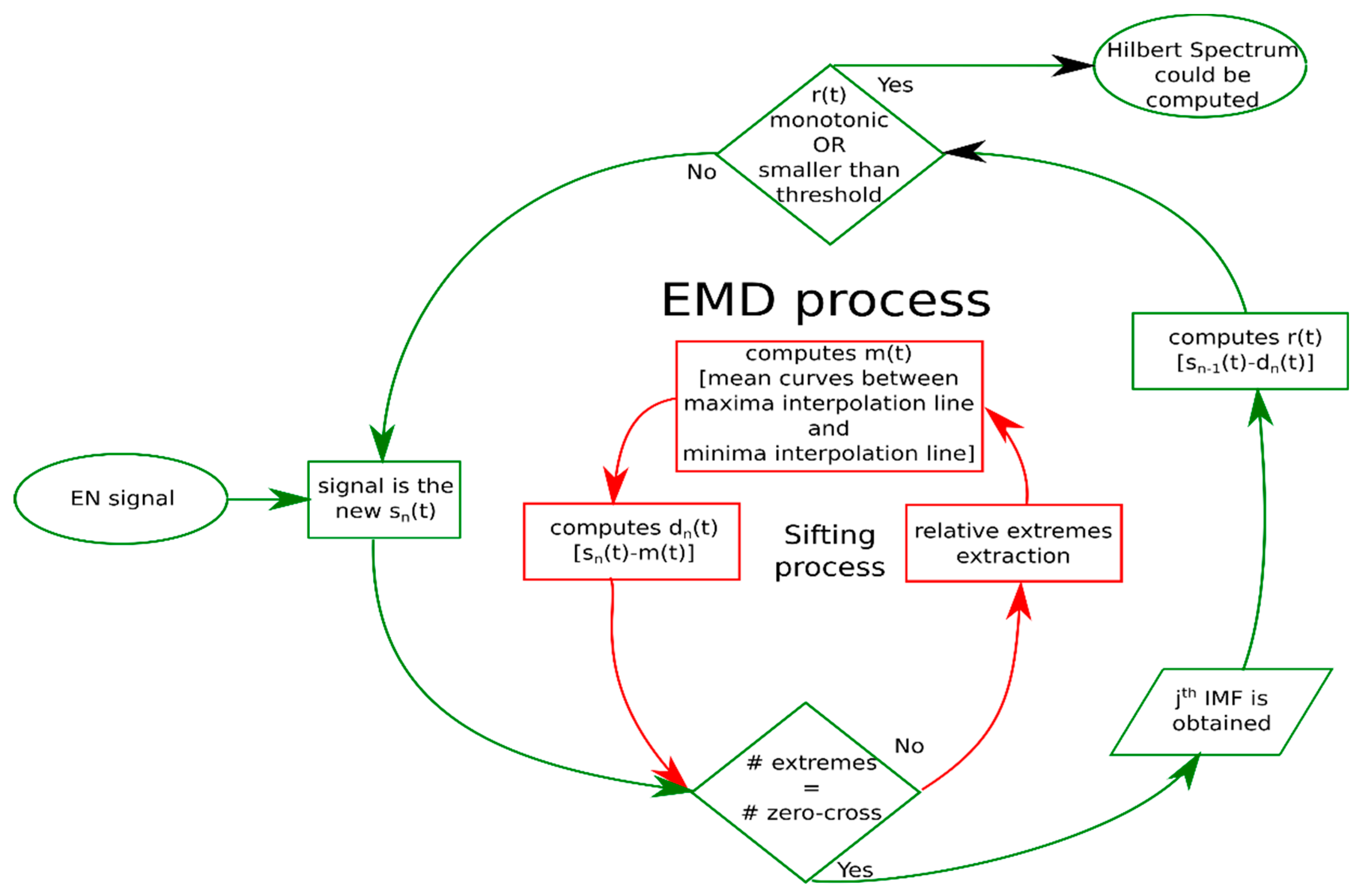
2.2. Hilbert–Huang Transform Approach

HHT is a way to analyse the signal through its Intrinsic Mode Functions (IMFs). The IMFs run in a simple oscillatory mode with varying amplitude and frequency along a time axis [35,36], and are used to obtain instantaneous frequencies at each moment in time with a symmetrical wave profile. The decomposition of the signal into its IMFs is obtained using the Empirical Mode Decomposition (EMD) method.

Empirical Mode Decomposition (EMD) [29,36] is an empirical method that exploits the definition of IMF to carry out the decomposition: a function with an equal number (or with a difference of 1) of extremes and zero crossing, whose envelopes are symmetric with respect to zero (i.e., at any point the average of the signal envelope determined by the local maxima and the envelope determined by the local minima is zero). It represents a generally simple oscillatory mode.

So, the EMD algorithm is composed by two indented processes: the main process and the sifting process. The main process is performed via the following steps, which are applied to the signal s(t):

• Executing the sifting process on the s(t), obtaining an IMF denominated as d_n(t).
• Calculating the residual r(t) = s_n−1(t) − d_n(t) (then, this residual is considered a new s(t)).

The sifting process consists of the following steps:

• Extracting relative extremes, obtaining two functions: v₁(t) is the interpolation of the maxima point, and v₂(t) is the interpolation of the minima point
• Determining the m(t) function as m(t) = 1/2(v₁(t) + v₂(t))
• Extracting d(t) = s(t) − m(t)

The sifting process is iterated i-times, until the number of extreme values equals the number of zero-crossings. The main process is iterated N-times, until r(t) is a monotonic function or r(t) is smaller than a predefined threshold.

Therefore, the original signal is decomposed as:

$$\mathrm{s}\left(\mathrm{t}\right)=\left(\sum _{\mathrm{n}=1}^{\mathrm{N}}{\mathrm{d}}_{\mathrm{n}}\left(\mathrm{t}\right)\right)+{\mathrm{r}}_{\mathrm{N}}(\mathrm{t})$$

(1)

By means of this method, each data set, however complex, can be decomposed into a finite number of components, each of which meets the definition of IMF. In Figure 3, the developed EMD algorithm is schemed. All algorithms have been implemented in Python language (Python 3.11.4).

The EMD method operates in the time domain, and it is highly efficient and very adaptive [37]. It furnishes a holomorphic function that is suitable to be used with the well-known Hilbert Transform (HT) to produce an accurate description of the signal. Hilbert Spectral Analysis (HSA) is then applicable to examine each IMFs as functions of time. The result is a frequency–time distribution of signal amplitude, named the Hilbert Spectrum, permitting the analysis of localized features [38]. The Hibert Spectrum thus provides an accurate resolution in punctual time, instead of averaging over the entire dataset of a time-window.

3. Results and Discussion

3.1. Time Domain Analysis

In Figure 4, the time series of the electrochemical noise potential and current, after a polynomial de-trend, are shown (Figure 4a,b, respectively). Polynomial de-trending is a type of filtering method that is widely used to remove trends in ENC and ENP signals [39]. It entails approximating the trend using a polynomial of a given order m. The coefficients of the polynomial were identified using the least squares regression method. An m = 5 polynomial order was chosen. According to [40], this choice is a good computational compromise, since the change of noise resistance in m > 4 can be considered negligible, implying that a high m order of the polynomial is not required. Furthermore, m > 6 values are advised to avoid large computed mistakes and relevant variations at the start and end of the data. Moreover, with high m, Rn exhibits extremely irregular variations after drift removal.

EN potential, after polynomial de-trend, shows a low-frequency fluctuation at increasing time, with amplitude ranging from 10 mV to 20 mV. The potential oscillations are relatively large and wide with usually about 4000 s periodicity (point A in Figure 4a), although a constancy of this parameter is not clearly identifiable. Occasionally, mainly at longer times, some large fluctuations can be also observed (point B in Figure 4a).

Current noise signal, after polynomial de-trend, is described by low-frequency broad fluctuations overlaid to high-frequency abrupt fluctuation with quick decay. At a low testing time, a series of small transient current peaks (repeated periodically in the whole transient) are observed (point C in Figure 4b); the majority of them are defined by a wide increase followed by a sharp reduction, which is said to be particularly prevalent during metastable pitting of stainless steels alloys [41,42,43] because of the slow growth of the pit, and prompt depassivation.

After about 1500 s, new transient phenomena, characterized by a sharp rise and a relatively short decay, were recorded (point D in Figure 4b). These events showed very high currents at, approximately, every 10–20 s, which suggests they were linked to the damage process of pits turning into cracks [44].

The third stage, at a longer testing time, is distinguished by a substantially large transient with a very sluggish decline. (point E in Figure 4b).

Considering the long duration of the acquired data and the significant fluctuations in frequency and amplitude ranges both on voltage and current transients, a visual time-domain analysis could not achieve a simple discrimination of several corrosion stages that take place during a SCC phenomenon [45].

However, in order to be able to acquire information related to the mode and stages of damaging mechanisms on SCC tests, electrochemical and statistical parameters from electrochemical noise data can be extrapolated. Several variables can be used to make a description of the corrosion phenomena, some of which derive from a time domain analysis, such as the standard deviation of noise potential and current, noise resistance, localization index, etc [46].

Noise Resistance, R_N, is described as the ratio of the standard deviation of potential and current variation.

$${\mathrm{R}}_{\mathrm{N}}=\frac{{\mathsf{\sigma }}_{\mathrm{E}}}{{\mathsf{\sigma }}_{\mathrm{I}}}$$

(2)

The Localization Index, LI, [47,48] is a variable that is related to the type of corrosion taking place: generalized (value close to 0) or localized (value close to 1). It has been demonstrated that this variable is very sensitive to electrode asymmetry [49]. It is calculated as:

$$\mathrm{L}\mathrm{I}={\mathsf{\sigma }}_{\mathrm{I}}/\sqrt{{\mathrm{I}}_{\mathrm{n}\mathrm{o}\mathrm{i}\mathrm{s}\mathrm{e}}^2+\overline{{\mathrm{I}}^2}}$$

(3)

where I_noise corresponds to the electrochemical noise current signal, I to the mean value, and σ_I to the standard deviation of the I_noise signal.

Another approach aimed to analyse EN signal, based on the shot noise theory, is based on the concept that current noise signals may be thought of as charge packets (with certain limitations [50]). Using the equations that come next, the charge associated with every electrochemical event, q, and the event frequency, f_n, may be calculated from the potential and current noise signals, according to [51]:

$$\mathrm{q}=\frac{\sqrt{{\mathsf{\psi }}_{\mathrm{E}}}\sqrt{{\mathsf{\psi }}_{\mathrm{I}}}}{\mathrm{B}}$$

(4)

$${\mathrm{f}}_{\mathrm{n}}=\frac{{\mathrm{B}}^2}{{\mathsf{\psi }}_{\mathrm{E}}\mathrm{A}}$$

(5)

where ψ_E and ψ_I are the low-frequency PSD values of the potential and current noise, respectively, B is the Stern–Geary coefficient (0.026 V [50]), and A the exposed electrode area (24.1 cm²). The charge q gives an indication of the lost metal mass in the event, while f_n provides information about the frequency of these events [51].

The charge, q, is considered to be an affordable index of the localized corrosion activity [48,52], so the cumulative sum of the charge could be used as an index to evaluate the overall rate of electrochemical noise activities that take place on the specimen surface.

In order to use the previously mentioned set of variables, a sliding window method was used. Each window has a width of 10 min and an overlap of 60 s. Window dimension and overlapping were chosen in such a way to ensure a sufficient resolution to the variable q.

The cumulative charge–time evolution is reported in Figure 5. By analysing this trend, it is possible to detect a first region, up to 1500 s of stability, where no significant electrochemical activity was observed. This stage could be related with the pre-activation corrosion phase. After that, the cumulative charge increases, showing a progressive enhancement of the electrochemical activity on the specimen surface. Figure 6 confirms this by showing the evolution during the time of the current standard deviation. The spikes represent an increased variability in current signal, related with electrochemical event occurrence. The first significant peak, point A in Figure 6, occurs around 1000 s. This local current peak could be ascribed to the activation of metastable pits. Therefore, this phase can be related to electrochemical phenomena activation on the specimen surface. Therefore, the relevant step in the cumulative charge rate observed at about 1500 s may be associated with the activation and propagation of surface pits (point B in Figure 5).

Then, at an increased time, a reduction of the electrochemical activity occurred, leading to the observation of a plateau with only some smooth steps in the cumulative charge plot (point B’ in Figure 5). In this stage, in the range 1500–10,000s, a relevant variability of the current standard deviation takes place, with intermediate peaks and valley regions (point C Figure 6).

After approximately 10,000 s, a progressive rise of the cumulative charge trend takes place until sample failure occurs. Continuous fluctuations in the standard deviation trend with relevant peak values occur (points C in Figure 6), and are related to short to long range cracks propagation [53]. In this stage, analysing the cumulative charge trend, continuous steps of increase and stabilization of the electrochemical activity can be identified (points C in Figure 5). Compatible with that in [14], this behaviour could be associated with the SCC cracks propagation. Due to the increase in crack length, the stress concentration increases at the crack tip, causing it to undergo more widespread blunting. A bigger plastic area means a longer period for the fracture to be reshaped by dissolution in order for a new crack to propagate [54]. Hence, crack stabilization periods, where metal dissolution (and, therefore, electrochemical activity) is relevant, are coupled cyclically with crack evolution (related to low electrochemical activity) [55].

With the advancing of crack length, the steps, point B and B’ in Figure 5, increase in height as a consequence of the progressive transition from short to long range crack propagation (magnitude from 0.6 nC to 2.7 nC). Afterward, for times above 40,000–45,000 s, the cumulative charge increases monotonically with short deviations from linearity (points C’ in Figure 5). This period is the prelude of the final rupture of the sample that takes place after about 58,000 s.

Concerning this, different EN features (e.g., noise resistance, localization index, etc.), are usually applied as key parameters to detect localized corrosion [48,56]. This is also applicable to a complex corrosive mechanism such as SCC [18]. Details of the main statistical parameter of the ENC and ENP time series investigated in this paper are reported in [14]; however, usually it is required to take a multiple variable approach on EN features, e.g., by using a neural network method [14], to discriminate the fundamental parameters and their correlation during the different and synergistic phases of the process. Surely, the integration of all this information can represent a profitable approach to investigate the phenomena which evolves during the SCC. However, this requires support validation of frequency or time-frequency domain analysis.

3.2. Frequency Domain Analysis

With the purpose of better highlighting the differences in the EN signals during the SCC damage steps, frequency domain analysis was performed.

Due to the application hypotheses at the basis of the Fourier Transform, for a correct use of the FFT algorithm, a signal framing was performed. The size of the signal framing windows was chosen in order to have signal portions that are stationary and linear. This approach has the benefit to obtain combined time and frequency information, i.e., a non-native representation for the Fourier Transform.

Due to the non-deterministic nature of the EN signals, based on FFT spectra, the PSD graph results in a more suitable analysis. This approach uses the auto-correlation function of the recorded signal, so it is capable to extract information about the signal power, but, at the same time, loses all the information based on the phase.

In Figure 7, the time evolution of PSD of the current signal is reported. As shown in the graph, different phases, each of which could be related to the corrosion phases, are difficult to detect. Several fluctuations in the initial and medium period of the test can be identified. Therefore, it is possible to perceive different activities which take place, but it is difficult to discriminate and relate each different stage to a specific corrosion phenomenon. This is due to the multiple variation in PSD parameters (roll-off slope, white noise, cut-off frequency, stop frequency, magnitude), which simultaneously occurs during time. Therefore, this discrimination activity is very difficult to be argued against via the conventional amplitude graph, due to the multivariate nature of the corrosion phenomena.

3.3. Time-Frequency Domain Analysis

The Wavelet transform has a strong theoretical base as in the case of FFT/PSD theory, but it adds native support to the non-stationary signals. In addition, it furnishes a native energy–time–frequency representation.

The mother wavelet function, applied here, is a Ricker wavelet (also known as the Mexican hat wavelet) [57], with a scale depth of 30. The scale parameter is inversely proportional to the frequency parameter.

Figure 8 shows the Continuous Wavelet Transform applied to the EN current signal. A mixed time scale was performed. In particular, in order to better evidence all corrosion evolution stages during the SCC test, a log-time scale at a short time, and a linear scale at a longer time were utilised.

Similarly to PSD analysis, the graph analysis shows the presence of different signal stages (detected by different magnitude at different scale). This analysis is advantageous, and enables us to obtain a better time resolution due to the absence of the approximation induced by the critical choice of the temporal window size which afflicts the STFT algorithm.

The Wavelet Transform cannot overcome the limitations related to the non-linearity of the signal. In addition, it has some inaccuracies related to the frequency resolution. Moreover, the choice of the mother wavelet turns out to be very critical. Despite these limitations, it is possible to make an interpretation of the electrochemical phenomena in progress during the SCC test.

According to the stages detected by the univariate analysis, the graph was divided in three stages. At first, up to about 1500 s, a growing electrochemical activity can be noticed. This area of activity shows a peak at the medium frequency range, and, as time increases, a widening of the peak towards the low frequencies is shown. A second phase, in the range 1500–5000 s, is characterized by the presence of competitive mechanisms, respectively, at medium-high and medium-low frequencies, followed by, at around 5000–10,000 s, an electrochemical quiescence zone. This region can be related to the triggering and mechanical propagation of the short-range cracks [14].

Afterwards, starting from 10,000 s and coded as the SCC short to long range crack propagation phase, according to Figure 5, more relevant electrochemical activities take place. This region is characterized by several subclusters of current transient signals, which are depicted by high magnitude and a scale frequency of about 10³ Hz. These regions identify that, at this stage, the propagation phenomenon by SCC is due to electrochemical contribution. Furthermore, the continuous alternation between high-intensity peaks and areas of lower relevance, compatible with the presence of transition mechanisms between stabilization due to local plastic deformation and long range crack propagation, are slightly visible. This last phase turns out to be preparatory to the final failure. Consequently, although this technique is able to discriminate the pit triggered SCC phase with relative sub-steps, it does not allow effective discrimination of the long-range crack propagation stages by providing partial information on the damage evolution in this phase.

A further improvement could be provided by the fractional energy of smooth and low-frequency crystals in wavelet analysis to better identify the corrosion mode (general, metastable or stable pitting) and its start time in the sample during the corrosion phenomenon [58]. By comparing the energy ratio of each crystal in the data sets, it could be possible, based on the power of WA, to distinguish corrosion types and assess their severity [59].

The Hilbert–Huang Transform (HHT), performed via the empirical mode decomposition (EMD) approach, was proposed to investigate the damage corrosion steps from the acquired EN non-stationary and non-periodic data. The EMD algorithm decomposes the original signal in its Intrinsic Mode Functions (IMFs): functions that respect the application condition of the Hilbert Transform.

The crack advancement rate, according to the SCC phenomenon, should be constant during the subcritical crack advancement phase. Certainly, given the interdependence of stress corrosion cracking growth rates, as determined by an integration of crack tip mechanics and crack tip oxidation kinetics [60], a suitable forecast for the influence of K on stress corrosion cracking growth rate is possible on these phenomena, and therefore could provide an improvement in knowledge regarding this concern. At first, the current approach is to evaluate, based on the ENC and ENP transient, how the electrochemical events are modified and how using a time-frequency technique (such as HHT), it is possible to identify macro-features of the process that are able to better discriminate, compared to conventional techniques, the phenomena for their correlation with the damage evolution steps in SCC.

In Figure 9, the results of the EMD decomposition for the current noise signal are shown. Only the first eight IMFs are presented. The current electrochemical noise was used for the HHT analysis, due to its powerful representation of corrosion phenomena compared to the potential signal.

The EN current signal has been decomposed into eleven IMFs. The IMFs that are characterized by a non-flat phase and an amplitude with a constant mean value are the most significant ones. IMFs that are characterized by a higher amplitude (and consequently greater power amount) includes large energy information of the source signal. A large number of IMFs (from the 6th to the 11th ones) are characterized by a very low amplitude and frequency (very close to the DC component) spectrum. Thus, these IMFs can probably be related to slow fluctuation phenomena (e.g., temperature, solution conductivity, etc). Consequently, only the first five IMFs can be considered relevant to the study of the corrosion phenomenon.

In Figure 10, the first IMF of the electrochemical noise current data is represented. The first IMF represents the most significant contributor to the whole signal and to the Hilbert Spectrum analysis, either in amplitude and in frequency content contribution.

It is possible to identify regions in which the activity is remarkably clear, interspersed with other regions where the quiescence of the electrochemical activity is noted.

In particular, identifying the stages in which the amplitude magnitude of the first current IMF has major peaks, four time steps can be identified:

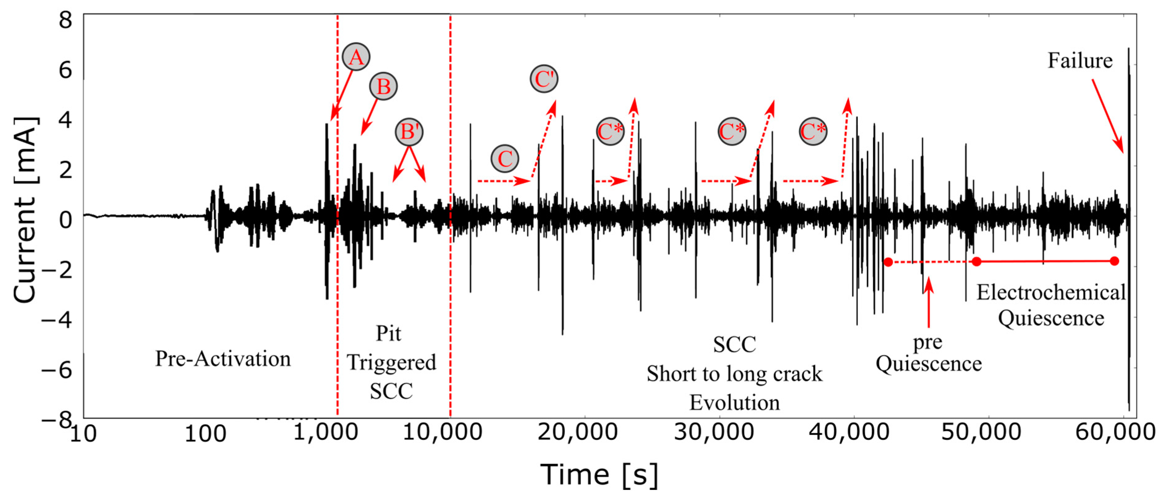
• At first, up to 1500 s, a low electrochemical activity region can be identified. As previously discussed, this stage could be related with the pre-activation corrosion phase. At very short times the electrochemical activity is not representative. However, with increasing time, the intensity of the IMF progressively increases. The first intensity and wide peak, point A in Figure 10, occurs at about 1000 s, in correspondence with the triggering of metastable pits [61]. Consequently, this phase can be associated with the superficial electrochemical activation of the specimen [62].
• The pre-activation stage continues to evolve during time, with the presence of several sub-peaks (point B in Figure 10), up to about 2000 s, in correspondence with the activation and propagation of superficial pits. Subsequently the IMF signal undergoes a sharp reduction in intensity, during which there are only occasional signal spikes (point B’ in Figure 10). During this time, in the time interval 2000–10,000 s, predominantly, the pit-to-crack transition takes place. The triggering of the SCC phenomenon obviously stimulates the defect evolution partly by mechanical contribution making therefore the electrochemical one less significant. The occasional secondary IMF peaks, identified by point B’, may be associated with the local formation and propagation of additional surface pits that evolve simultaneously during the stress corrosion triggering phase.
• After about 10,000 s a third stage was defined as short to long range crack propagation can be identified. During this stage several fluctuations in IMS signal can be highlighted. In particular After a long electrochemical quiescence step (point C in Figure 10) a significant peak can be identified at about 16,000–18,000 s (point C’ in Figure 10). This trend related to stabilization and abrupt increase steps in IMF noise current signal is periodically identifiable. This behaviour is caused by the crack evolution by SCC [36]. At this stage, the size of the crack can reach a length sufficient to assume that the stress concentration at the crack tip becomes significant, thus implying that there is a large area of plastic deformation, leading to a more extensive blunt at the crack tip. Due to the crack reshape, the mechanical crack evolution mechanism is inhibited, despite electrochemical dissolution [48]. Consequently, a phase of electrochemical stabilization associated with the mechanical evolution of SCC damage is complementary to a phase of metal dissolution at the crack tip, and, therefore, complementary to an electrochemical activity phase. Depending on various electrochemical dissolution factors, the current transient generated by the micro-crack opening and re-passivation can last for a few seconds [63]. These sub-steps alternate cyclically during this stage (points C* in Figure 10), where the sub-critical propagation of the medium and long-range crack takes place.
• After about 45,000 s, after a transient region (coded as pre-quiescence), a large electrochemical plateau in the IMF signal can be identified (above 48,000 s). During this step, no relevant electrochemical vents can be identified. This stage is the prelude for the critical failure of the sample that took place after about 58,000s.

In order to be able to better discriminate the different time steps with significant electrochemical activity, it may be desirable to relate each time step with both amplitude and frequency of each IMF.

In Figure 11, the Hilbert transform of the entire electrochemical noise current signal is shown. This graph represents the trend of the frequency content vs. time.

The Hilbert Spectra allow to discriminate events occurring in different time instants with high precision, as well as facilitating the identification and characterization of these phenomena. Figure 11 can be used as a topological map by highlighting different clustered areas of the map, and relating them to specific degradation phenomena that take place during the SCC test. Each cluster in the map is defined as a homogeneous area characterized by similar frequency contents.

Based on these considerations, four main cluster areas can be identified:

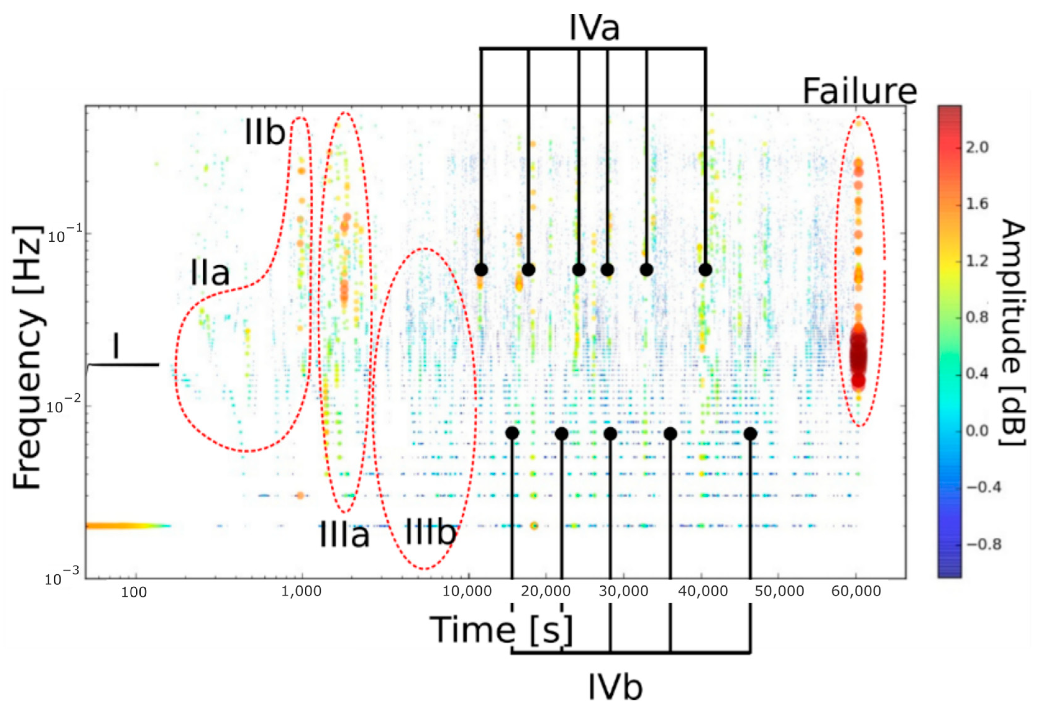
• Stabilization: at first, in the rage 0–100 s (step I in Figure 11), the noise signal is not characterised by any significant fluctuations. EN transient related to this phenomenon is characterised by the absence of high-frequency events: only some events at about 10⁻³ Hz can be observed. In this phase, the interaction between the electrolyte and specimen surface takes place, with an unstable alternation of general corrosion and passivation phases. The aggressive ions locally destabilize the passive oxide layer of the sample, causing a local thinning of the oxide. This process has a short duration (approximately 100 s) due to the high aggressiveness of the environment conditions of the test.
• Electrochemical activation: in the range 100–1500 s (step II in Figure 11), in correspondence with depassivated surface regions, the electrochemical activity is enhanced and the pit initiation stage extends to micrometre-sized, large dissolved holes. In this phase, an increase in the cumulative charge trend was also identified. This sub-stage is identified by a high activity at medium and low frequencies. In particular, at increasing time (after about 500 s) and with a progressive increment in the number of pits on the surface, the signal activity evolves towards a higher frequency (from 2 × 10⁻² to 5 × 10⁻¹ Hz, defining two substep: IIa and Iib). This stage can be related with the electrochemical activation phase (Iia) and the subsequent triggering of metastable pits (Iib) on the sample surface [14].
• SCC Activation and Propagation: This region, ranging from 1500 to 10,000 s, can be related mainly with the SSC triggering by short range crack activation. At this stage, the electrochemical activity becomes significant. Some sub-clusters can be identified. At first, region IIIa, as shown in Figure 11, suggests that high-frequency contribution can be identified. At this stage, the aggressive ions locally destabilize the passive oxide layer of the sample, causing a local thinning of the oxide. In correspondence with depassivated surface regions, the electrochemical activity is enhanced and the pit initiation stage extends to micrometre-sized, large dissolved holes (see pit in Figure 12d). This process leads to the formation of preferential areas of localized attacks by pitting, identifiable by a high magnitude of the IMF. Progressively, the signal activity evolves towards a lower frequency (from 5 × 10⁻³ to 5 × 10⁻² Hz) and magnitude (from 10^0.4 to 10^−0.4 dB), as shown via region IIIb in Figure 11. In this low frequency phase, the mechanical contribution is more relevant than the electrochemical one, as evidenced by the low EN signal magnitude, indicating that SCC short-range activation of the cracks was triggered [14].
• SCC propagation. At about 10,000 s, a new step begins. During this step, the SCC damage evolution phase of the sample occurs (in Figure 12c, it is possible to note a secondary crack originating from a pit). The progressive crack growth (region III) leads to an increase in the region of plastic deformation at the crack tip [64]. This implies that a more severe anodic dissolution is needed by the crack to re-sharpen before inducing a further propagation. At this phase, in fact, the dissolution within the crack is still taking place. When increasing the crack length, an increase in stress concentration occurs, which induces a larger plastic zone ahead of the crack tips. As a result, the crack point becomes more blunted. A larger plastic zone suggests that it will take more time for the fracture to be re-sharpened via dissolving for future crack propagation. This phase was indeed indicated as a mechanical quiescence [53] and the driving force in crack propagation. This stage shows metal dissolution at the crack tip. This region could correspond to the high-frequency activity in the first IMF. The electrochemical dissolution (sub-steps IVa in Figure 11), identifiable via the step-wise increase in cumulative charge (Figure 5), stimulates the mechanical instability of the crack (sub-steps IVb in Figure 11), primed for future subsonic propagation. Consequently, this stage identifies the prelude to the catastrophic failure of the specimen. In the topological map, this region is identified by medium-low amplitude valleys alternating with high-frequency peaks (5 × 10⁻²–3 × 10⁻¹ Hz). Afterwards, for times above 45,000 s, the Hilbert spectrum shows a low magnitude region where an electrochemical quiescence occurs. Finally, for catastrophic failure, the sample takes place after about 58,000s.

From a morphological point of view, the specimen’s fracture surface was irregular, showing mixed ductile/brittle propagation modes (Figure 12a), and confirmed the previous argument in relation to analysing the data in Figure 11. Cracks began with a cleavage-like manner from the pit’s bottom (point A, B and C in Figure 12a). A detail of a reference-pitted cracked area is shown in Figure 12b, where the short-range crack propagation by cleavage mechanisms is identifiable. In Figure 12d, a surface illustration of a pit to crack progression is depicted (stage III in Figure 11). The corrosion is caused by random germinating open-hemispherical holes with diameters of around 20 μm on the surface of the samples, as well as the gradual initiation and propagation of river-shaped fractures with the pit as their origin. Moreover, for long-distance cracks, ductile crack propagation can occur in conjunction with the crack apex due to localized plastic deformation at the crack tip (dotted ellipse in Figure 12d). Figure 12c depicts further information on crack propagation mechanism in relation to the dog-bone gauge cross section. The crack started from superficial pit and then propagated in a branched trans-granular mode.

On the basis of the above reported considerations, it can be possible to divide the HHT spectrum into specific damage mechanism areas, according to the schematic representation shown in Figure 13, in which we can distinguish SCC short- and long-range crack evolution and failure stages. The possibility to have topological maps is a further advantage of the HHT method, providing a graphical support in order to better discriminate the significant evolving damage phases.

Concerning the SCC short-range evolution stage, a crack activation cluster can be identified. This cluster is characterized by sharp peaks due to local corrosion attacks on the sample surface (pitting). Instead, the low-frequency region is related to short-range mechanical crack growth. Analogously, several sub-steps can be identified via analysing the SCC short-to-long-range evolution stage. EN events characterized by high magnitude and high frequency are clustered, and able to identify the dissolution of the crack tip’s metal. All events at low frequency identify the transition of the crack growth from short-to-long-range propagation. This transition is also related to a modification from brittle (cleavage) to ductile in crack evolution (as valuable in Figure 12). This region is usually related with a mechanistic SCC quiescence phase [65]. Afterwards, at a longer time, the electrochemical quiescence phase can be considered as a precondition for the final catastrophic failure of the sample.

In conclusion, it is the author’s opinion that HHT algorithms and the related Hilber–Huang Spectrum are powerful instruments for analysing non-stationary and non-linear signals of an EN data set, which overcomes the theoretical limits of Fast Fourier and Wavelet transforms. In these particular instances, the use of EN measurements not only validated earlier ideas established from time and frequency analysis, but also allowed the identification of multiple SCC damage processes happening over time on stainless steel samples. This separation was accomplished by the establishment of correlations between key EN properties and the relevant damage mechanisms.

Considering that, in SCC, the effects of the electrochemical reaction and mechanical stress occur simultaneously, a combined approach of the two techniques can be considered effective. In several papers [14,66,67], it was possible to detect how the combination of an electrochemical technique (EN) with a mechanistic one (e.g., acoustic emission, AE), by means of neural network analysis, can be profitable in order to determine the key features of the SCC process and the evolutionary states of damage. With this in mind, a future scope will be the possibility to synergistically combine the EN technique, analysed by means of HHT, with the acoustic emission technique by integrating them through neural network analysis.

4. Conclusions

The EN technique was used to investigate the SCC damage evolution on 17-4PH stainless steel samples. The conventional methods (time and frequency domain analysis) showed promising results on predicting the damage phase. However, they require a complex interpretation of the results, due to the system’s multivariate nature. Furthermore, the theoretical assumptions involve some approximations when applied to the EN signals.

For this purpose, the HHT method, based on an empirical mode decomposition (EMD) approach, allows calculating and analysing the EN signal accurately. This ability to handle and process non-stationary and non-linear data results in a detailed representation of the signal contents in the time–frequency domain.

Using the technique, clear information was obtained about the transitions between different corrosion phases caused by the SCC test. It was possible (i) to identify a specific response to each corrosion damage phenomenon, (ii) determine the timeline with accuracy, and (iii) also provide a topological representation of the SCC damage stages as they evolved.

In particular, the following stages were detected:

• Stabilization: at first, in the rage 0–100 s. The EN transient is characterised by the absence of high-frequency events. Only some events at about 10⁻³ Hz were observed.
• Electrochemical activation: in the range 100–1500 s. This stage was identified by a high activity at medium and low frequencies (from 2 × 10⁻² to 5 × 10⁻¹ Hz,). This stage can be related with electrochemical activation and the subsequent triggering of metastable pits on the sample surface.
• SCC Activation and Propagation: ranging from 1500 to 10,000 s. This is mainly related to the SSC triggering by short-range crack activation. At this stage, the electrochemical activity became significantly identifiable by a high magnitude of IMF. Then, progressively, the signal activity evolved towards a lower frequency (from 5 × 10⁻³ to 5 × 10⁻² Hz) and magnitude (from 10^0.4 to 10^−0.4 dB), because the mechanical contribution was more relevant than the electrochemical.
• SCC propagation. Above 10,000 s. This is related to progressive crack growth. This region was identified by medium–low amplitude valleys alternating with high-frequency peaks (5 × 10⁻²–3 × 10⁻¹ Hz). For times above 45,000 s a low magnitude region, related to an electrochemical quiescence, was identified before catastrophic failure of the samples.

These results indicate the HHT method as a potentially powerful technique for EN signal processing. Additionally, HHT is able to recognize and distinguish different damage mechanism stages that occur during degradation.

References

1. Benavides, S. Corrosion Control in the Aerospace Industry; Woodhead Publishing: Cambridge, UK, 2009. [Google Scholar]
2. Rao, B.P.C.; Raj, B. NDE Methods for Monitoring Corrosion and Corrosion-Assisted Cracking. In Non-Destructive Evaluation of Corrosion and Corrosion-Assisted Cracking; John Wiley & Sons, Inc.: Hoboken, NJ, USA, 2019; pp. 101–121. ISBN 9781118987735. [Google Scholar]
3. Calabrese, L.; Proverbio, E. A Review on the Applications of Acoustic Emission Technique in the Study of Stress Corrosion Cracking. Corros. Mater. Degrad. 2021, 2, 1–30. [Google Scholar] [CrossRef]
4. Cai, W.; Jomdecha, C.; Zhao, Y.; Wang, L.; Xie, S.; Chen, Z. Quantitative Evaluation of Electrical Conductivity inside Stress Corrosion Crack with Electromagnetic NDE Methods. Philos. Trans. R. Soc. A Math. Phys. Eng. Sci. 2020, 378, 20190589. [Google Scholar] [CrossRef] [PubMed]
5. Xia, D.-H.; Song, S.-Z.; Behnamian, Y. Detection of Corrosion Degradation Using Electrochemical Noise (EN): Review of Signal Processing Methods for Identifying Corrosion Forms. Corros. Eng. Sci. Technol. 2016, 51, 527–544. [Google Scholar] [CrossRef]
6. Lv, J.; Yue, Q.; Ding, R.; Wang, X.; Gui, T.; Zhao, X. The Application of Electrochemical Noise for the Study of Metal Corrosion and Organic Anticorrosion Coatings: A Review. ChemElectroChem 2021, 8, 337–351. [Google Scholar] [CrossRef]
7. Xia, D.-H.; Song, S.; Behnamian, Y.; Hu, W.; Cheng, Y.F.; Luo, J.-L.; Huet, F. Review—Electrochemical Noise Applied in Corrosion Science: Theoretical and Mathematical Models towards Quantitative Analysis. J. Electrochem. Soc. 2020, 167, 081507. [Google Scholar] [CrossRef]
8. Xia, D.-H.; Deng, C.-M.; Macdonald, D.; Jamali, S.; Mills, D.; Luo, J.-L.; Strebl, M.G.; Amiri, M.; Jin, W.; Song, S.; et al. Electrochemical Measurements Used for Assessment of Corrosion and Protection of Metallic Materials in the Field: A Critical Review. J. Mater. Sci. Technol. 2022, 112, 151–183. [Google Scholar] [CrossRef]
9. Lau, K.; Permeh, S. Assessment of Durability and Zinc Activity of Zinc-Rich Primer Coatings by Electrochemical Noise Technique. Prog. Org. Coat. 2022, 167, 106840. [Google Scholar] [CrossRef]
10. Obot, I.B.; Onyeachu, I.B.; Zeino, A.; Umoren, S.A. Electrochemical Noise (EN) Technique: Review of Recent Practical Applications to Corrosion Electrochemistry Research. J. Adhes. Sci. Technol. 2019, 33, 1453–1496. [Google Scholar] [CrossRef]
11. Zhang, Z.; Yuan, X.; Zhao, Z.; Li, X.; Liu, B.; Bai, P. Electrochemical Noise Comparative Study of Pitting Corrosion of 316L Stainless Steel Fabricated by Selective Laser Melting and Wrought. J. Electroanal. Chem. 2021, 894, 115351. [Google Scholar] [CrossRef]
12. Hoseinieh, S.M.; Homborg, A.M.; Shahrabi, T.; Mol, J.M.C.; Ramezanzadeh, B. A Novel Approach for the Evaluation of Under Deposit Corrosion in Marine Environments Using Combined Analysis by Electrochemical Impedance Spectroscopy and Electrochemical Noise. Electrochim. Acta 2016, 217, 226–241. [Google Scholar] [CrossRef]
13. Xia, D.-H.; Ma, C.; Behnamian, Y.; Ao, S.; Song, S.; Xu, L. Reliability of the Estimation of Uniform Corrosion Rate of Q235B Steel under Simulated Marine Atmospheric Conditions by Electrochemical Noise (EN) Analyses. Measurement 2019, 148, 106946. [Google Scholar] [CrossRef]
14. Calabrese, L.; Bonaccorsi, L.; Galeano, M.; Proverbio, E.; Di Pietro, D.; Cappuccini, F. Identification of Damage Evolution during SCC on 17-4 PH Stainless Steel by Combining Electrochemical Noise and Acoustic Emission Techniques. Corros. Sci. 2015, 98, 573–584. [Google Scholar] [CrossRef]
15. Zhao, R.; Xia, D.-H.; Song, S.-Z.; Hu, W. Detection of SCC on 304 Stainless Steel in Neutral Thiosulfate Solutions Using Electrochemical Noise Based on Chaos Theory. Anti-Corros. Methods Mater. 2017, 64, 241–251. [Google Scholar] [CrossRef]
16. Wei, Y.-J.; Xia, D.-H.; Song, S.-Z. Detection of SCC of 304 NG Stainless Steel in an Acidic NaCl Solution Using Electrochemical Noise Based on Chaos and Wavelet Analysis. Russ. J. Electrochem. 2016, 52, 560–575. [Google Scholar] [CrossRef]
17. Calabrese, L.; Galeano, M.; Proverbio, E.; Di Pietro, D.; Donato, A.; Cappuccini, F. Advanced Signal Analysis of Acoustic Emission Data to Discrimination of Different Corrosion Forms. Int. J. Microstruct. Mater. Prop. 2017, 12, 147–164. [Google Scholar] [CrossRef]
18. Carmona-Hernández, A.; Orozco-Cruz, R.; Carpio-Santamaria, F.A.; Campechano-Lira, C.; López-Huerta, F.; Mejía-Sánchez, E.; Contreras, A.; Galván-Martínez, R. Electrochemical Noise Analysis of the X70 Pipeline Steel under Stress Conditions Using Symmetrical and Asymmetrical Electrode Systems. Metals 2022, 12, 1545. [Google Scholar] [CrossRef]
19. Benzaid, A.; Huet, F.; Jérôme, M.; Wenger, F.; Gabrielli, C.; Galland, J. Electrochemical Noise Analysis of Cathodically Polarised AISI 4140 Steel. I. Characterisation of Hydrogen Evolution on Vertical Unstressed Electrodes. Electrochim. Acta 2002, 47, 4315–4323. [Google Scholar] [CrossRef]
20. Li, X.; Liu, C.; Zhang, T.; Lv, C.; Liu, J.; Ding, R.; Gao, Z.; Wang, R.; Liu, Y. Effect of PH and Applied Stress on Hydrogen Sulfide Stress Corrosion Behavior of HSLA Steel Based on Electrochemical Noise Analysis. J. Iron Steel Res. Int. 2023. [Google Scholar] [CrossRef]
21. van der Merwe, J.W.; du Toit, M.; Klenam, D.E.P.; Bodunrin, M.O. Prediction of Stress-Corrosion Cracking Using Electrochemical Noise Measurements: A Case Study of Carbon Steels Exposed to H2O-CO-CO2 Environment. Eng. Fail. Anal. 2023, 144, 106948. [Google Scholar] [CrossRef]
22. Jáquez-Muñoz, J.M.; Gaona-Tiburcio, C.; Cabral-Miramontes, J.; Nieves-Mendoza, D.; Maldonado-Bandala, E.; Olguín-Coca, J.; Estupinán-López, F.; López-León, L.D.; Chacón-Nava, J.; Almeraya-Calderón, F. Frequency Analysis of Transients in Electrochemical Noise of Superalloys Waspaloy and Ultimet. Metals 2021, 11, 702. [Google Scholar] [CrossRef]
23. Oppenheim, A.V.; Schafer, R.W.; Buck, J.R. Discrete Time Signal Processing; Prentice-Hall: Edinburg, Scotland, 1999; Volume 1999, ISBN 0137549202. [Google Scholar]
24. Rhif, M.; Ben Abbes, A.; Farah, I.R.; Martínez, B.; Sang, Y. Wavelet Transform Application for/in Non-Stationary Time-Series Analysis: A Review. Appl. Sci. 2019, 9, 1345. [Google Scholar] [CrossRef]
25. Jacobsen, E.; Lyons, R. The Sliding DFT. IEEE Signal Process. Mag. 2003, 20, 74–80. [Google Scholar] [CrossRef]
26. Allen, J.B. Short Term Spectral Analysis, Synthesis, and Modification by Discrete Fourier Transform. IEEE Trans. Acoust. Speech Signal Process. 1977, 25, 235–238. [Google Scholar] [CrossRef]
27. Zhang, Z.; Li, X.; Zhao, Z.; Bai, P.; Liu, B.; Tan, J.; Wu, X. In-Situ Monitoring of Pitting Corrosion of Q235 Carbon Steel by Electrochemical Noise: Wavelet and Recurrence Quantification Analysis. J. Electroanal. Chem. 2020, 879, 114776. [Google Scholar] [CrossRef]
28. Huang, N.E.; Wu, Z. A Review on Hilbert-Huang Transform: Method and Its Applications. October 2008, 46, 1–23. [Google Scholar] [CrossRef]
29. Huang, N.E.; Shen, Z.; Long, S.R.; Wu, M.C.; Shih, H.H.; Zheng, Q.; Yen, N.-C.; Tung, C.C.; Liu, H.H. The Empirical Mode Decomposition and the Hilbert Spectrum for Nonlinear and Non-Stationary Time Series Analysis. Proc. R. Soc. A Math. Phys. Eng. Sci. 1998, 454, 903–995. [Google Scholar] [CrossRef]
30. Calabrese, L.; Galeano, M.; Proverbio, E. Identifying Corrosion Forms on Synthetic Electrochemical Noise Signals by the Hilbert–Huang Transform Method Hilbert–Huang Transform Method. Corros. Eng. Sci. Technol. 2018, 53, 492–501. [Google Scholar] [CrossRef]
31. Homborg, A.M.; van Westing, E.P.M.; Tinga, T.; Zhang, X.; Oonincx, P.J.; Ferrari, G.M.; de Wit, J.H.W.; Mol, J.M.C. Novel Time-Frequency Characterization of Electrochemical Noise Data in Corrosion Studies Using Hilbert Spectra. Corros. Sci. 2013, 66, 97–110. [Google Scholar] [CrossRef]
32. Jáquez-Muñoz, J.M.; Gaona-Tiburcio, C.; Cabral-Miramontes, J.; Nieves-Mendoza, D.; Maldonado-Bandala, E.; Olguín-Coca, J.; López-Léon, L.D.; Flores-De los Rios, J.P.; Almeraya-Calderón, F. Electrochemical Noise Analysis of the Corrosion of Titanium Alloys in NaCl and H2SO4 Solutions. Metals 2021, 11, 105. [Google Scholar] [CrossRef]
33. Moradi, M.; Rezaei, M. Electrochemical Noise Analysis to Evaluate the Localized Anti-Corrosion Properties of PP/Graphene Oxide Nanocomposite Coatings. J. Electroanal. Chem. 2022, 921, 116665. [Google Scholar] [CrossRef]
34. Cottis, R.A. 5—Electrochemical noise for corrosion monitoring. In Techniques for Corrosion Monitoring; Woodhead Publishing: Cambridge, UK, 2001. [Google Scholar] [CrossRef]
35. Delgadillo, R.M.; Tenelema, F.J.; Casas, J.R. Marginal Hilbert Spectrum and Instantaneous Phase Difference as Total Damage Indicators in Bridges under Operational Traffic Loads. Struct. Infrastruct. Eng. 2023, 19, 824–844. [Google Scholar] [CrossRef]
36. Huang, N.E. An Adaptive Data Analysis Method for Nonlinear and Nonstationary Time Series: The Empirical Mode Decomposition and Hilbert Spectral Analysis. In Applied and Numerical Harmonic Analysis; Birkhäuser Verlag: Basel, Switzerland, 2006. [Google Scholar] [CrossRef]
37. Li, Y.; Lin, J.; Niu, G.; Wu, M.; Wei, X. A Hilbert–Huang Transform-Based Adaptive Fault Detection and Classification Method for Microgrids. Energies 2021, 14, 5040. [Google Scholar] [CrossRef]
38. Zhang, Z.; Zhao, Z.; Bai, P.; Li, X.; Liu, B.; Tan, J.; Wu, X. In-Situ Monitoring of Pitting Corrosion of AZ31 Magnesium Alloy by Combining Electrochemical Noise and Acoustic Emission Techniques. J. Alloys Compd. 2021, 878, 160334. [Google Scholar] [CrossRef]
39. Lentka, Ł.; Smulko, J. Methods of Trend Removal in Electrochemical Noise Data–Overview. Measurement 2019, 131, 569–581. [Google Scholar] [CrossRef]
40. Havashinejadian, E.; Danaee, I.; Eskandari, H.; Nikmanesh, S. Investigation on Trend Removal in Time Domain Analysis of Electrochemical Noise Data Using Polynomial Fitting and Moving Average Removal Methods. J. Electrochem. Sci. Technol. 2017, 8, 115–123. [Google Scholar] [CrossRef]
41. Hu, J.; Deng, J.; Deng, P.; Wang, G. Corrosion Monitoring Method of 304 Stainless Steel in a Simulated Marine–Industrial Atmospheric Environment: Electrochemical Noise Method. Anti-Corros. Methods Mater. 2022, 69, 629–635. [Google Scholar] [CrossRef]
42. Kearns, J.R.; Scully, J.R.; Roberge, P.R.; Reichert, D.L.; Dawson, J.L. Electrochemical Noise Measurement for Corrosion Applications-STP 1277; ASTM International: Philadelphia, PA, USA, 1996. [Google Scholar]
43. Gabrielli, C.; Huet, F.; Keddam, M.; Oltra, R. Review of the Probabilistic Aspects of Localized Corrosion. Corrosion 1990, 46, 266–278. [Google Scholar] [CrossRef]
44. Calabrese, L.; Galeano, M.; Proverbio, E.; Di Pietro, D.; Donato, A. Topological Neural Network of Combined AE and EN Signals for Assessment of SCC Damage. Nondestruct. Test. Eval. 2020, 35, 98–119. [Google Scholar] [CrossRef]
45. Ramezanzadeh, B.; Arman, S.Y.; Mehdipour, M.; Markhali, B.P. Analysis of Electrochemical Noise (ECN) Data in Time and Frequency Domain for Comparison Corrosion Inhibition of Some Azole Compounds on Cu in 1.0 M H2SO4 Solution. Appl. Surf. Sci. 2014, 289, 129–140. [Google Scholar] [CrossRef]
46. Fabre-Pulido, J.; Orozco-Cruz, R.; Mejía-Sánchez, E.; Contreras-Cuevas, A.; Galvan-Martinez, R. Stress Corrosion Cracking Process of X60 Steel Immersed in a Brine Solution with Corrosion Inhibitor through the Electrochemical Noise Technique. ECS Trans. 2019, 94, 189. [Google Scholar] [CrossRef]
47. Nagiub, A.M. Comparative Electrochemical Noise Study of the Corrosion of Different Alloys Exposed to Chloride Media. Engineering 2014, 6, 1007–1016. [Google Scholar] [CrossRef]
48. Cottis, R.A.; Al-Awadhi, M.A.A.; Al-Mazeedi, H.; Turgoose, S. Measures for the Detection of Localized Corrosion with Electrochemical Noise. Electrochim. Acta 2001, 46, 3665–3674. [Google Scholar] [CrossRef]
49. Mansfeld, F.; Sun, Z. Technical Note: Localization Index Obtained from Electrochemical Noise Analysis. Corrosion 1999, 55, 915–918. [Google Scholar] [CrossRef]
50. Sanchez-Amaya, J.M.; Cottis, R.A.; Botana, F.J. Shot Noise and Statistical Parameters for the Estimation of Corrosion Mechanisms. Corros. Sci. 2005, 47, 3280–3299. [Google Scholar] [CrossRef]
51. Cottis, R.A. Interpretation of Electrochemical Noise Data. Corrosion 2001, 57, 265–284. [Google Scholar] [CrossRef]
52. Permeh, S.; Lau, K. Identification of Steel Corrosion Associated with Sulfate-Reducing Bacteria by Electrochemical Noise Technique. Mater. Corros. 2023, 74, 20–32. [Google Scholar] [CrossRef]
53. Calabrese, L.; Campanella, G.; Proverbio, E. Identification of Corrosion Mechanisms by Univariate and Multivariate Statistical Analysis during Long Term Acoustic Emission Monitoring on a Pre-Stressed Concrete Beam. Corros. Sci. 2013, 73, 161–171. [Google Scholar] [CrossRef]
54. Shaikh, H.; Amirthalingam, R.; Anita, T.; Sivaibharasi, N.; Jaykumar, T.; Manohar, P.; Khatak, H.S. Evaluation of Stress Corrosion Cracking Phenomenon in an AISI Type 316LN Stainless Steel Using Acoustic Emission Technique. Corros. Sci. 2007, 49, 740–765. [Google Scholar] [CrossRef]
55. Nguyen, T.-T.; Bolivar, J.; Shi, Y.; Réthoré, J.; King, A.; Fregonese, M.; Adrien, J.; Buffiere, J.-Y.; Baietto, M.-C. A Phase Field Method for Modeling Anodic Dissolution Induced Stress Corrosion Crack Propagation. Corros. Sci. 2018, 132, 146–160. [Google Scholar] [CrossRef]
56. Tan, Y. Sensing localised corrosion by means of electrochemical noise detection and analysis. Sens. Actuators B Chem. 2009, 139, 688–698. [Google Scholar] [CrossRef]
57. Ganjalizadeh, V.; Meena, G.G.; Wall, T.A.; Stott, M.A.; Hawkins, A.R.; Schmidt, H. Fast Custom Wavelet Analysis Technique for Single Molecule Detection and Identification. Nat. Commun. 2022, 13, 1035. [Google Scholar] [CrossRef]
58. Kim, J.J. Wavelet Analysis of Potentiostatic Electrochemical Noise. Mater. Lett. 2007, 61, 4000–4002. [Google Scholar] [CrossRef]
59. Smith, M.T.; Macdonald, D.D. Wavelet Analysis of Electrochemical Noise Data. Corrosion 2009, 65, 438–448. [Google Scholar] [CrossRef]
60. Shoji, T.; Lu, Z.; Murakami, H. Formulating Stress Corrosion Cracking Growth Rates by Combination of Crack Tip Mechanics and Crack Tip Oxidation Kinetics. Corros. Sci. 2010, 52, 769–779. [Google Scholar] [CrossRef]
61. Homborg, A.M.; Tinga, T.; Zhang, X.; van Westing, E.P.M.; Oonincx, P.J.; Ferrari, G.M.; de Wit, J.H.W.; Mol, J.M.C. Transient Analysis through Hilbert Spectra of Electrochemical Noise Signals for the Identification of Localized Corrosion of Stainless Steel. Electrochim. Acta 2013, 104, 84–93. [Google Scholar] [CrossRef]
62. Guan, L.; Zhang, B.; Yong, X.P.; Wang, J.Q.; Han, E.-H.; Ke, W. Effects of Cyclic Stress on the Metastable Pitting Characteristic for 304 Stainless Steel under Potentiostatic Polarization. Corros. Sci. 2015, 93, 80–89. [Google Scholar] [CrossRef]
63. Zhang, Z.; Wu, X. Interpreting Electrochemical Noise Signal Arising from Stress Corrosion Cracking of 304 Stainless Steel in Simulated PWR Primary Water Environment by Coupling Acoustic Emission. J. Mater. Res. Technol. 2022, 20, 3807–3817. [Google Scholar] [CrossRef]
64. Calabrese, L.; Galeano, M.; Proverbio, E.; Di Pietro, D.; Cappuccini, F.; Donato, A. Monitoring of 13% Cr Martensitic Stainless Steel Corrosion in Chloride Solution in Presence of Thiosulphate by Acoustic Emission Technique. Corros. Sci. 2016, 111, 151–161. [Google Scholar] [CrossRef]
65. Aoyagi, Y.; Kaji, Y. Crystal Plasticity Simulation Considering Oxidation along Grain Boundary and Effect of Grain Size on Stress Corrosion Cracking. Mater. Trans. 2012, 53, 161–166. [Google Scholar] [CrossRef]
66. Kawasaki, Y.; Fukui, S.; Fukuyama, T. Phenomenological Process of Rebar Corrosion in Reinforced Concrete Evaluated by Acoustic Emission and Electrochemical Noise. Constr. Build. Mater. 2022, 352, 128829. [Google Scholar] [CrossRef]
67. Kovac, J.; Alaux, C.; Marrow, T.J.; Govekar, E.; Legat, A. Correlations of Electrochemical Noise, Acoustic Emission and Complementary Monitoring Techniques during Intergranular Stress-Corrosion Cracking of Austenitic Stainless Steel. Corros. Sci. 2010, 52, 2015–2025. [Google Scholar] [CrossRef]
Figure 1. Scheme of SCC test setup.
Cmd 04 00034 g001
Figure 2. Scheme of EN damage analysis procedure.
Cmd 04 00034 g002
Figure 3. Schematic representation of EMD algorithm. # indicates the analysed numbers.
Cmd 04 00034 g003
Figure 4. Electrochemical noise of potential (ENP) (a) and current (ENC) (b) vs. time.
Cmd 04 00034 g004
Figure 5. Normalized Charge Cumulative trend. A coupled log-linear time scale is performed, in order to evidence the short time segment.
Cmd 04 00034 g005
Figure 6. Current Standard Deviation evolution during time. A coupled log-linear time scale is performed in order to evidence the short time segment.
Cmd 04 00034 g006
Figure 7. Time evolution of the Power Spectral Density related to the current EN signal. The coloured bar indicates PSD amplitude [A2Hz−1].
Cmd 04 00034 g007
Figure 8. Continuous Wavelet Transform applied to the EC current signal. A non-linear time scale is performed in order to evidence the low time characteristics. A coupled log-linear time scale is performed in order to evidence the short time segment.
Cmd 04 00034 g008
Figure 9. EMD algorithm applied to the current noise signal. (a) original current signal. (b,c): obtained IMFs (1 to 8).
Cmd 04 00034 g009
Figure 10. Hilbert–Huang Transform applied to the electrochemical noise current data: only the first IMF is shown. A coupled log-linear time scale is performed in order to evidence the short time segment.
Cmd 04 00034 g010
Figure 11. Hilbert Spectrum representation: up: 3D view, down: Frequency/Time contour plot. A coupled log-linear time scale is performed in order to evidence the short time components.
Cmd 04 00034 g011
Figure 12. SEM-SE morphology of the fracture surface, details (ac). Cracks began in a cleavage pattern from the pit’s bottom. The specimen’s final rupture was identified by ductile propagation. Furthermore, gauge cross section displaying a pit-originating fracture (Vilella’s reagent etch) (d).
Cmd 04 00034 g012
Figure 13. Damage steps in Hilbert Spectrum Map.
Cmd 04 00034 g013