Article

Evaluating the Impact of Redox Potential on the Corrosion of Q125, 316L, and C276 Steel in Low-Temperature Geothermal Systems

Department of Geology and Geography, West Virginia University, 98 Beechurst Ave., Morgantown, WV 26506, USA
*
Author to whom correspondence should be addressed.
Corros. Mater. Degrad. 2023, 4(4), 573-593; https://doi.org/10.3390/cmd4040030
Submission received: 5 September 2023 / Revised: 25 September 2023 / Accepted: 2 October 2023 / Published: 8 October 2023

Abstract

:
Time series experiments were used to explore the fluid redox impact on the corrosion of Q125, 316L, and C276 steels in low-ionic-strength and neutral water at temperature and pressure conditions associated with low-temperature geothermal systems. After exposing polished samples of each steel grade to an oxidizing (H2O2) and a reducing (Zn-doped) fluid for intervals of 24 h, 1 week, and 6 weeks, the atomic force microscopy results revealed general corrosion for Q125, while 316L and C276 exhibited pitting, crevice expansion, and edge attack corrosion. Secondary depositional features are frequently found as topographic highs, adjacent to pitting corrosion. These features may be identified as there is a very strong spatial correlation between the height retrace and phase retrace surface maps. All steels became progressively rougher over time after exposure to both fluids, while the corrosion rates were more complex. Samples exposed to the reducing fluid experienced an increase in the corrosion rate over time, while C276 and 316L experienced a decrease in the corrosion rate. Finally, a novel data validation technique was developed to address the intrinsic scalability of corrosion. The results indicate that the AFM scan area does not affect the measured surface roughness over nearly three orders of magnitude.

1. Introduction

Corrosion investigations that are explicitly designed for geothermal applications often involve various combinations of the following conditions: a relatively high temperature [1,2,3,4], an acidic pH [5,6,7], and supercritical CO2 levels [8,9], across a range of different grades of steel in a brine which is often modeled based on specific geothermal fields [2,4,6]. These contributions are valuable, but the complexity and number of the variables that are present can make it difficult to identify general trends. In one instance, a multivariate approach was taken, although the mild steel was of no specific grade [10]. In general, corrosion is more significant in fluids with higher ionic strength and acidity compared to fluids with low ionic strength, or those of neutral or alkaline pH (e.g., [11]). Moreover, while higher temperatures increase the reaction kinetics, it is unclear how reasonably well corrosion data that are obtained at one temperature may be extrapolated to another. Finally, the importance and relationship of O2 and H2 are complex. Oxygen can serve as an electron acceptor and thus aid in corrosion. For example, oxygen scavengers are introduced in the well to mitigate dissolved oxygen-induced corrosion in the oil and gas industry [12]. However, O2-rich fluids have been shown to form a protective oxide coating, slowing corrosion, relative to H2-rich fluids [13].
Geothermal energy is often harnessed from fluids with temperatures of >200 °C [14]. Recently, however, there has been an interest in lower temperature (T < 100 °C) deep direct use (DDU) systems. [15] Some corrosion studies have been performed at relatively low geothermal temperatures (<100 °C); however, these studies involved complex brine chemistries with commensurate high ionic strengths [2,3]. Furthermore, considering that geothermal fluids are highly varied, with some fields having ionic strengths of ~10−3 molal [16], we find that the primary control of fluid redox at a combined low temperature and ionic strength is unknown. Such conditions are suited for the consideration of DDU geothermal systems.
Atomic force microscopy (AFM) is a high-resolution technique that has been used for nanometer-scale corrosion analysis [17]. It has been employed in many base metal or steel corrosion studies (e.g., [18,19,20,21,22]). AFM is an excellent analytical instrument for corrosion studies where parameters such as the surface roughness are sought.
The goal of this study is to constrain the complexity of steel corrosion by comparing the effects induced after exposure to an initially reducing fluid to the effects produced by an initially oxidizing fluid. By normalizing the pressure and temperature, along with ionic strength minimization, the experimental conditions model the reinjection side of a surficial, low-temperature geothermal power plant. Evaluating the degree of corrosion across multiple grades of steel in these relatively unaggressive conditions may also place a lower constraint on the corrosion rates and behavior of the steels, since the corrosion effects are expected to be enhanced at higher temperatures, ionic strengths, and acidic conditions.
As this research will show, steel corrosion is possible even in quite unaggressive conditions, and that the fluid pH and Eh evolve considerably over time. In addition, some outstanding questions that are raised include whether the minor sulfur content in the steel is sufficient to promote pitting corrosion. Also, the results and analysis below indicate that surface roughness is largely spatially indifferent over approximately three orders of magnitude, although the upper limit of this insensitivity is unknown.

2. Materials and Methods

2.1. Steel and Fluid Preparation

Three grades of steel (Q125, 316L, and C276) were selected because of their widespread use at or near the reinjection point of geothermal power plants (Table 1). 316L and C276 were chosen because they are common steel grades found in the corrosion literature, which serve as a valuable basis of comparison to delineate the role of Eh. 316L and C276 steel bars, approximately 6 mm in diameter, were sectioned into smaller pieces, about 16 to 18 mm in length. In addition, Q125 steel was chosen because it is a type of steel with a high tensile strength and is used as a well-casing material, suitable for deep direct use (DDU) geothermal systems. Q125 steel was obtained from a drilling operator as a 14 cm diameter pipe. To remove the curvature of the steel pipe that was required for the AFM analysis and provide a similar surface geometry to that of the 316L and C276 pieces, the Q125 steel pieces were milled into rectangular prisms, measuring approximately 15 × 15 × 6 mm. A total of six steel pieces were milled (each steel grade in duplicate) and prepared for two sets of batch reactions with the corrosive fluid.
All sectioned steel pieces were polished using an Allied High Tech Multiprep polisher in the Shared Research Facilities at West Virginia University. This polisher was equipped with diamond lapping films and polished all steel samples to a mirror finish (≤1 µm). Polishing increases the sample surface homogenization and reduces the surface roughness of the steel, thereby providing a basis for comparison before and after exposure to the corroding fluid. Finally, the polishing lubricant was removed (degreased) with acetone, rinsed with DI water, dried, and weighed. The composition of each steel is provided in Table 1. Note that the density of Q125 is not readily available and was determined via volume displacement to be ~7.8 g/cm3.
Stocks of both corroding fluids were made using 18.2 MΩ MQ water. To evaluate the Eh-induced corrosion, care was taken to minimize the ionic strength of each fluid. To this end, the low-Eh fluid (subsequently referred to as Fluid 1) was doped with 250 g of Zn metal (>99% purity ACS grade), with a calculated ionic strength of 0.0001 mol/L. The redox potential of Fluid 1 was monitored over the span of two weeks until the rate of change was minimized and the lowest ORP value was obtained. The raw ORP values were temperature-corrected and converted to SHE for reporting. The day before the start of the exposure testing, the Eh of Fluid 1 was −0.04 V. The high-Eh fluid (subsequently referred to as Fluid 2) consisted of a 6% (H2O2) solution with a calculated ionic strength of <0.0005 mol/L. Hydrogen peroxide was favored over a sodium hypochlorite solution (e.g., [28]) to avoid Na+ or Cl2 in the solution, which would increase the ionic strength of the fluid. Fluid 2 was made fresh on the day of the start of the exposure testing to limit its interaction with the atmosphere. The Eh of Fluid 2 was 0.3105 V at the beginning of the exposure tests. To eliminate the effect of the initial pH, both fluids were pH balanced using KOH to a value of 7.

2.2. Exposure Testing

One 250 mL Wheaton glass screw-top bottle was used for each grade of steel for each fluid. The steel pieces were placed into the Wheaton bottles, exposing the generalized region of interest (ROI) on the polished side. For Fluid 1, the 1500 mL stock fluid container was shaken to suspend any Zn particulates before filling each Wheaton bottle to 180 mL. The bottles were capped and placed onto a pre-heated hotplate (without stirring) at 75 °C, a temperature that is frequently associated with geothermal power plant reinjection in low-enthalpy systems [29,30]. Three time points (excluding t0) were selected at intervals of 24 h (t0–t1), 168 h (1 week) (t1–t2), and 1008 h (6 weeks) (t2–t3). At each time point, a ~60 mL aliquot of the fluid was filtered at 0.2 μm, acidified to 1%~v/v with concentrated trace metal grade HNO3, and the ORP and pH of the fluid was measured. The steel pieces were removed from the Wheaton vials, rinsed with DI water, dried, weighed, and photographed prior to the AFM analysis. The Wheaton bottles with the remaining fluid were kept on the hotplate at 75 °C for continuity. After the AFM analysis, the steel pieces were returned to the same Wheaton bottle, containing the remaining 75 °C fluid, until the next time point. While opening the reaction bottles at each time point for sampling would expose the fluid to atmospheric O2, this approach is not a flaw in the experimental design because binary power plants may be air-cooled, so it is representative of actual conditions [31]. After the first time series, the Wheaton bottles were allowed to soak in 10% HCl for over an hour, before triplicate DI rinsing before reuse. For the exposure tests using Fluid 2, each of the Wheaton bottles were wrapped in aluminum foil to reduce the H2O2 degradation.

2.3. Atomic Force Microscopy

Atomic force microscopy was performed using an Asylum MFP-3D, located in the Shared Research Facilities at West Virginia University. The steel samples were loaded onto glass slides with the probe tip above the polished region on the steel surface (aided by identifying the inscribed arrow indicators) and analyzed in the AC air topography mode. The instrument was retuned for each new steel sample, and if the retracted free amplitude varied by more than |0.05 A| from the set amplitude throughout the analytical session. The selected ROIs were typically 50 × 50 μm or 90 × 90 μm in area, with the latter being the maximum size allowed by the instrument. This scan size was chosen to collect spatial information over the largest area possible to maximize the sample representation. Multiple topographic maps were made in the polished region of each steel piece at each time point. The data were processed (i.e., graphical representation and surface roughness (Sa)) using the software program, Gwyddion.

3. Results

The average AFM topographic data and mass loss corrosion rate are presented in Table 2 for all steels, timepoints, and fluids. The mass loss corrosion rate was calculated at each time point following the form given by Mundhenk et al. (2013) [6]. If the change in mass was not measurable (i.e., below the LOD), the corrosion rate was incalculable; this does not necessarily mean that zero corrosion occurred, however. Here, we assume that the steel density and surface area did not change and were held constant. Therefore, uncertainty was principally controlled by the dimensional imprecision of the steel pieces. The dimensions for each steel sample piece were measured to the nearest mm (±0.5 mm). This level of accuracy results in ~9%, ~12%, and ~13% uncertainty for the corrosion rates for the Q125, 316L, and C276 steels, respectively. Polishing relics likely contribute to the surface roughness uncertainty at TP0 on all six steel samples. Interestingly, the higher grit 1 µm polish performed better than the 0.5 µm polish, as the 0.5 µm polishing produced surface roughness values of 30 ± 4 nm, 17 ± 32 nm, and 23 ± 15 nm for Q125, 316L, and C276, respectively, for the first batch used in the Fluid 1 exposure tests. In comparison, the second batch of steel samples used in the Fluid 2 exposure tests were polished to 1 µm, and yielded surface roughness values of 17 ± 11 nm, 15 ± 6 nm, and 15 ± 8 nm for Q125, 316L, and C276, respectively.

3.1. Fluid 1 (Low Eh) Exposure

Fluid 1 in each Wheaton bottle rapidly changed from a net reducing (Eh at TP 0 = −0.04 V) to an oxidizing fluid (~0.44 V) when exposed to all steel grades (Figure 1A). The pH of Fluid 1 remained relatively unchanged from TP0 to TP2. In the final time series, TP2–TP3, the pH of Fluid 1 increased by at least one unit for each steel grade, with an increasing rate of change over time (average pH/h of 6.9 × 10⁻⁴ for TP0 to TP1, −5.6 × 10⁻⁴ for TP1 to TP2, and 1.2 × 10⁻³ for TP2 to TP3). This observation, in conjunction with that made for the Eh, seems to support a protracted fluid evolution, and that Fluid 1 did not reach a steady state even after a combined total of 1200 h. Note that, while there was a decrease in the rates of change for both the pH and Eh from TP0 to TP1 and TP1 to TP2, this trend was reversed for the final TP2 to TP3 interval.
The surface roughness values for each steel sample progressively increased over time. It is worth noting that some localized surface features were interpreted as polishing relics (Figure 2 and Figure 3) and represent a source of uncertainty, as it is possible that some of these features may have been inadvertently included in the AFM analyses (Figure 4), resulting in potential false positives. Pitting corrosion is observed in all samples, while Q125 experiences general corrosion (Figure 3 and Figure 4). The Sa of each steel increased monotonically after each timepoint for the entire 1200 h duration.
The surface roughness of all steels became significantly rougher over the entire 1200 h exposure time (Figure 1D and Figure 4, Table 2). Q125 most notably displayed a relatively homogenous surface roughness increase compared to the other two grades of steel, where the significant increases in the surface roughness were more localized. Figure 4 displays the significantly oxidized surface at the end of the exposure. The entire surface of the Q125 steel underwent a general alteration (note that the AFM analysis was performed on the interior of the sample, as the rind was removed before analysis). Moreover, in some AFM topographic scans, the total translation exceeded the instrumental capability (~±7.5 µm). Fitting a logarithmic relationship to the corrosion rate data of Q125 (Figure 1C, Table 2) and taking the first derivative yields a corrosion rate that itself changes at (d2cm/dt2) = 2.7 × 10⁻⁷ cm/h2 (or 0.024 mm/year2). Pits formed on the surface of the 316L steel, and were frequently associated with adjacent peaks (Figure 3, TP 1 to 3). The surface roughness of 316L also became progressively rougher, and the average total vertical translation also increased, up to 1.8 µm after 1200 h exposure (Table 2). Long sequences of ~100 µm oblate pits in an echelon formation were produced, as well as an aggressive attack on the edges and corners, resulting in rounding and beveling (Figure 4). There was only one time interval in which a measurable mass loss was observed. Therefore, corrosion rate evolution analysis was not possible. C276 behaved similarly to 316L. Pits and immediately adjacent peaks were detected (e.g., Figure 3 TP2 for C276). This material generally experienced an increase in both the surface roughness and the total vertical translation over time, with the exception occurring at TP1, although both metrics were within uncertainty (Table 2). Like 316L, there were numerous gouges, as well as edge beveling and edge attacks, on the surface and corners of C276 (Figure 4). This steel did not experience a sufficient mass loss throughout the 1200 h exposure to allow for a mass loss corrosion rate, and because of this, it is impossible to even apply a constraint on the corrosion evolution of Fluid 1.

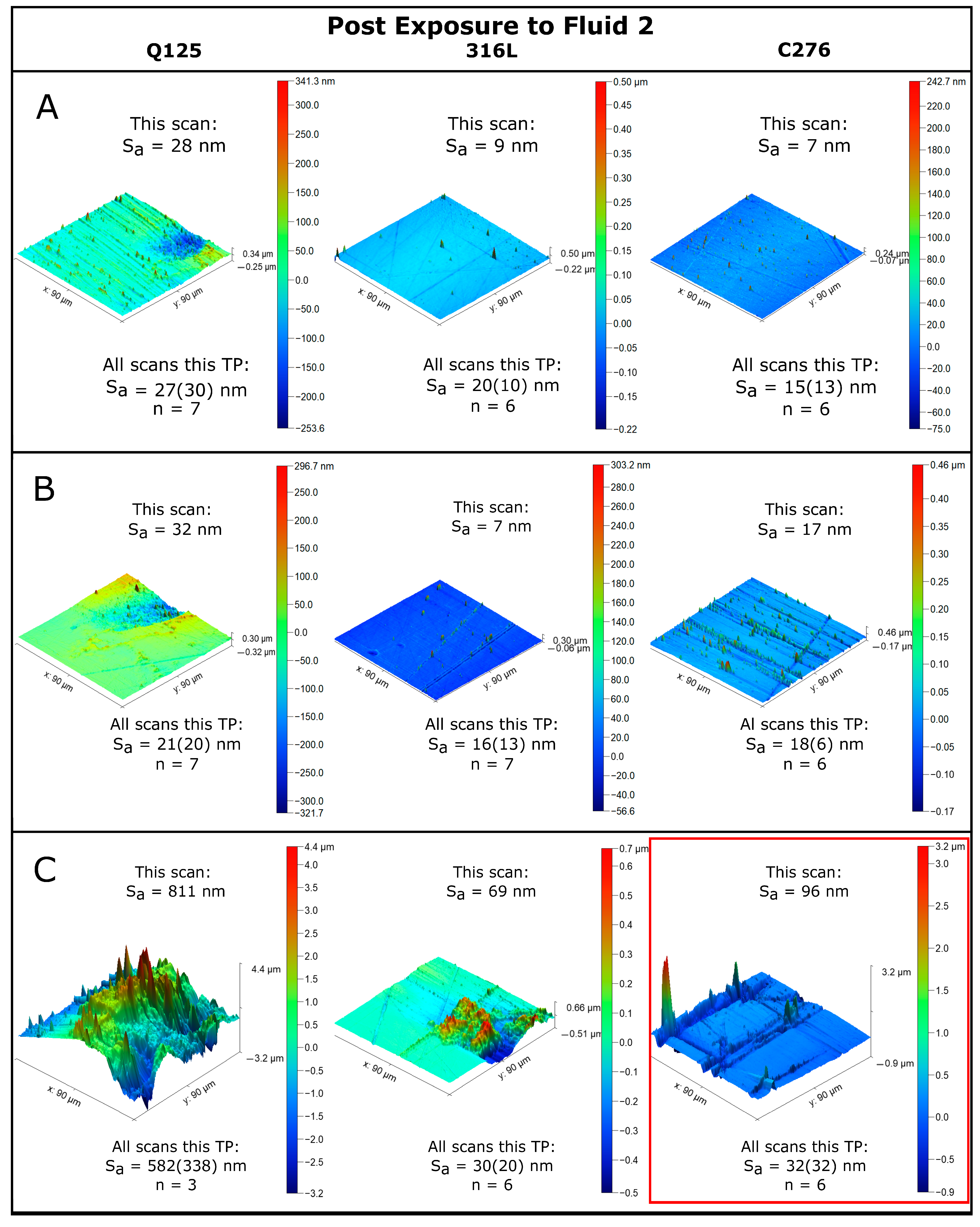
3.2. Fluid 2 (High Eh) Exposure

The pH and Eh evolution of Fluid 2 for all time points is given in Figure 5. After the exposure tests, the average pH values from all steel fluids increased by approximately 3 units from 7 to 9.5. Conversely, there was a decrease in the Eh of ~0.22 V, from 0.43 V to 0.216 V. The slope behavior of the pH versus time and Eh versus time were the same for all steel fluids across all time intervals. The rates of change for both parameters (dpH/dt and dEh/dt) were the greatest between TP0 and TP1. After TP1, the dpH/dt and dEh/dt progressively decreased over time. One interesting qualitative observation after the exposure of the steel samples to Fluid 2 was in their surface color. After a 24 h exposure (TP1), all steel samples were visually bright and had a shiny surface appearance. After TP2, the surface of C276 became an iridescent blue, but only for ~20 min before fading (Figure 6). Interestingly, this surface characteristic was retained after TP3 and did not diminish, and is contemporaneous with the golden-yellow corrosion feature (Figure 6). This area was targeted explicitly for AFM analysis (C276 TP3 is denoted by a red box in Figure 6 and Figure 7C). For the Q125 TP3 AFM data (Figure 7C), the exterior rind was gently removed prior to the AFM analysis of the interior. Finally, an audible gas release was noted after opening each Wheaton bottle for all timepoints, and gas bubbles were observed to be nucleating on the steel surfaces, particularly the C276 steel surface.
One of the most apparent observations of the C276 steel is the blue hue that was noticeable after TP2 (Figure 7). Regarding the surface features, there is a strong correlation between the linear features and the existence of ~100 µm tall peaks for the C276 steel (Figure 6, TP2). These features increased in frequency over time and were not observed in the pre-reaction AFM topographic maps. The pre-reaction AFM maps of the C276 steel contain similar or smaller ~100 µm peaks, but they are not as strongly correlated with valleys as in the post-reaction AFM topographic maps. This type of steel appears to display fissure expansion (red box in Figure 6 and Figure 7) and pitting corrosion. If the particularly rough localized corrosion (Figure 6 and Figure 7) is excluded, the surface roughness of the C276 steel samples changed minimally throughout the entire 1200 h exposure period (Table 2; if excluded, the surface roughness at TP3 becomes 20 ± 9 nm). Despite the overall small increase in the surface roughness of the C276 steel, a detectable mass loss was measured, allowing for a corrosion rate to be established, which decreased over time (Figure 5).
The mass loss corrosion rate and AFM data indicate that 316L performed similarly to C276, as the corrosion rate was also low and similarly decreased over time. Corrosion of the 316L steel at TP2 was not detected due to the mass loss being below detection. This does not, however, indicate that zero corrosion occurred in this time interval. Moreover, the surface roughness of 316L generally increased, although a decrease did occur at TP2, despite a total vertical translation increase of only 229 nm from TP0 to TP3 (Table 2). Regarding the corrosion type and surficial features, the 316L sample appears to have experienced significant pitting and edge attack (Figure 7).
The Q125 steel roughness increased significantly after TP2 at a rate of 0.56 nm/h, and in some instances, the vertical translation exceeded the capability of the AFM instrument (meaning that peaks or valleys on the surface had an absolute value > 7.5 µm). In contrast to the 316L and C276 steels, the Q125 steel experienced an acceleration in the corrosion rate despite similar pH and Eh fluid evolution behavior occurring in all three Wheaton aliquot bottles (Figure 5). At the start of the exposure test, this material experienced localized pitting, which transitioned into general corrosion at the end of the 1200 elapsed time. Similar to the rind encapsulating the Q125 piece from Fluid 1, the Q125 steel, after exposure to Fluid 2, produced a reddish-orange weathering rind (0.0861 g), which, after removal, accounted for 0.74% of the mass of the combined sample mass at TP0 (11.5931 g). Unfortunately, after the whole 1200 h exposure to Fluid 2, the corrosion was so extensive that the AFM tip broke, limiting the number of analyses to only three.

4. Discussion

4.1. Steel Grade Comparison

The Fe-rich Q125 steel performed the worst when exposed to both reducing (Zn-doped) fluid and oxidizing (H2O2) fluid, relative to 316L and C276. The effect of pre-existing surface roughness also plays a vital role in subsequent corrosion, as the unpolished Q125 steel surface is aggressively corroded, relative to the polished surface of the same sample (Fluid 1 in Table 2), indicating that a larger surface area for reactivity serves as positive feedback for corrosion. In respect of surface roughness, 316L performed slightly worse than C276 when exposed to reducing Fluid 1. When 316L was exposed to the oxidizing Fluid 2, the surface roughness was within uncertainty, and is thus statistically indistinguishable from the surface roughness observed on the C276 steel. The mass loss corrosion rates of 316L and C276 are similar between both materials and, in many cases, below the gravimetric balance’s detection limit. Note that this method is highly dependent upon sensitive balances and does not indicate that zero corrosion occurred. The Q125 steel corroded the fastest, at a rate of typically 102 greater than the other two steel grades. However, it is not immediately clear why the corrosion rate for Q125 increased when exposed to Fluid 1 and 2. However, there may be positive feedback with the transition from localized pitting to general surface corrosion. In this hypothesis, a rougher surface leads to more surface area, which leads to more corrosion nucleation sites, etc. Pitting corrosion is associated with the breakdown of the passivation layer and is exacerbated by the presence of halogen ions or thiosulfate [32]. The exact cause of this pitting, observed in all steel grades, is unknown, and is perplexing because, in the construction of the corroding fluids, neither halogen ions nor sulfur were introduced. However, each grade of steel does contain between 0.001 and 0.0272 wt % sulfur (Table 1). It remains to be shown whether or not this small amount of sulfur is capable of inducing localized pitting corrosion.
The ~20 min transient nature of the iridescent blue hue seen on the C276 steel sample suggests photosensitivity, while the long-term stability of the color after TP3 indicates a permanent coating. A blue hue has been noted on Cr-plated steel in the presence of low Cr-oxides, and was found to decrease in intensity as the Cr-oxides increased and took on a golden-tan color instead [33]. Therefore, the referenced work stands in strong agreement with the above observations, considering that the Eh evolution of Fluid 2 decreased over time, while the permanence of the iridescent blue hue increased. In addition, a blue/purple color (interpreted as a potential oxide) which transitions to yellow over time has been reported on alumina-forming austenitic steel [34]. It is thus likely that the golden-yellow corrosion feature occurring on the C276 surface at TP3 (Figure 7) may indicate what the potential surface of the steel would look like if the exposure time was further increased.

4.2. Fluid Comparison

In only 24 h of exposure to Fluid 2, C276 (regarded for its excellent corrosion resistance) experienced a measurable mass loss. Similarly, 316L and Q125 experienced 100% and 33% increases in mass loss in Fluid 2 at TP1 compared to Fluid 1. Considering the low ionic strengths and starting pH of 7, the effect of the more oxidizing fluid on corrosion is apparent. The oxidizing Fluid 2 induced more significant steel corrosion than the less-oxidizing Fluid 1, corroborating the aggressive bubbling that was observed on the steel surfaces submerged in Fluid 2. The decomposition of hydrogen peroxide into H2O and O2 is a spontaneous reaction [35], indicating that corrosive O2 will automatically be generated from Fluid 2 and attack the electron-rich steel surfaces. Moreover, one product in H2O dissociation is, of course, H+ (note that acidity may also increase in solution from CO2(g) partitioning into the fluid from the headspace in the unflushed/unevacuated Wheaton bottle). Merging two H+ yields molecular H2—a gas at the experiment pressure and temperature conditions. Indeed, H2 gas is produced and is the likely species of the observed gas bubbles [36], which bubble out of the solution, as observed, and simultaneously consumes acidity. Therefore, the positive pH evolution in Fluid 1 and 2 may be due to H+ consumption via the formation of H2 gas. This same phenomenon may explain the reversal of Eh values at TP3, because the H2O2 in Fluid 2 was converted into H+ and then reduced to H2(g). The gaseous H2 could not escape, but concentrated in the Wheaton bottle headspace instead. The increased partial pressure of hydrogen gas (pH2) resulted in an equilibration with the liquid in Fluid 2, allowing for partitioning back into the solution as H2(aq). This gas is reducing, and an increase in H2(aq) would cause the Eh of Fluid 2 to decrease.
The rapid change in the Eh values for Fluid 1 suggests that the reducing nature of the Zn-doped Fluid 1 was in disequilibrium with the atmospheric O2 in the Wheaton bottle. Interestingly, after only 24 h, the Eh values of Fluid 1 (mean = 0.442 V, all steels) and Fluid 2 (mean = 0.478 V, all steels) were very similar, suggesting that these fluids rapidly lost their initial redox characteristics and trended towards equilibrium. Yet, the pH remained the same (mean = 7.0 and 7.3, respectively). The pH,Eh coordinate pair for Fluid 1 at TP0 plots relatively close to the H2-H2O boundary while Fluid 2 plots in the center of the H2O field, indicating that Fluid 2 is likely more thermodynamically stable than Fluid 1. This may explain the sudden positive Eh excursion of Fluid 1 after only 24 h of exposure to a more stable pH,Eh coordinate, while also explaining why Fluid 2 deviated minimally after the same time interval. Over the entire 1200 h exposure test, both fluids likely approached equilibrium, as evidenced by the general decrease (or trend towards a rate of 0) for dEh/dt and dpH/dt. To ensure that the redox potentials of the fluid are maintained at disequilibrium values, this work could be improved by utilizing a reaction bottle that allows for both intermittent sampling and an evacuation or N2 flushing capability to remove atmospheric O2 (which promotes equilibrium).
Corrosion rates are dynamic and have been shown to both increase [2] and decrease [6] over time. While only the Q125 steel exhibited a measurable mass loss corrosion rate over multiple timepoints, Fluid 1 became slightly more corrosive over time. In comparison, all steels were corroded in Fluid 2, and the corrosivity of this fluid decreased over time. In summary, the corrosion results from the AFM surface roughness analysis, as well as the mass loss corrosion rates of steel when exposed to the oxidizing Fluid 2 solution, were greater than when exposed to Fluid 1.

4.3. Redepositional Features

Suspected redepositional features may be identified by comparing the height retrace and phase retrace AFM data (Figure 8). The latter is used to evaluate the boundaries between different materials on the basis of Van der Waals repulsive or attractive forces. Material phases that are ‘sticky’ will induce an attractive force on the AFM tip, resulting in a lag or offset (given in units of degrees) in the retrace map, relative to a non-sticky material. As can be seen in Figure 8, there is a strong spatial correlation between these two topographic maps, indicating that secondary corrosion products might be identifiable. Furthermore, the redepositional features appear to display a lower phase retrace angle, relative to the bulk steel substrate (Figure 8). Redepositional features are often located immediately adjacent to pitting corrosion, although, in other instances, they form amorphous topographical forms on the steel surface. The exact crystallography of the deposit is unknown, although they are likely oxy(hydroxides) [37] or hydroxides [4]. Crystallographic identification will inform the selective dissolution of the steel solid solution, relative to the corrosive fluid. For example, it has been shown that Zn increases in fluid at an acidic pH faster than Al [38]. To this end, we hypothesize that oxy(hydroxides) secondary deposits will have a lower phase retrace angle than the primary steel substrate, and that minerals such as wülfingite (Zn(OH)2) may be present, particularly in fluids or steels containing Zn.
Secondary products which form on the surface of steel offer corrosion protection, the result of which is a decrease in the corrosion rate [2]. Armoring peaks are not restricted to one steel grade or morphology. For example, on C276, the armoring peak is a prominent spire (Figure 8A), whereas on 316L, the armoring peak is immediately adjacent to the pitting corrosion (Figure 8B). These armoring peaks represent secondary precipitation from steel corrosion, reflecting a subtractive–additive relationship occurring at the fluid–steel interface. Like the fluid–rock interface in natural hydrothermal or geothermal systems, subtractive corrosion in one location may result in additive scaling in another. We propose that combining AFM phase retrace and height retrace data with a phase identification technique such as Raman spectroscopy (e.g., [37]) may further inform the corrosion-related fluid–steel interactions, thereby providing further information on the scale reduction of these secondary deposits.

4.4. Data Validation: Scale Dependence and Scan Window Model Selection

AFM, while being an excellent tool for corrosion imaging and topographic mapping, is limited in its spatial capability. Observations made in a particular ROI may or may not be representative at other sample surface locations. Using two different sub-window models (Figure 9), we sought to address surface area roughness scalability over nearly three orders of magnitude (from 25 µm2 to 8100 µm2). We have developed and herein introduced a repeating origin propagation (ROP) window model which uses the same starting point for each expanding sub-window (Figure 9A). In this model, the total scan area comprises several sub-windows of equal lengths. This model provides AFM data over the total scan area; however, each subsequent window propagation is affected by the previous windows’ data biasing, the effect of scale dependence, and surface heterogeneity. We also used the sliding origin propagation (SOP) window model, which provides wholly independent AFM data. The origin for the subsequent sub-window (xn,yn) is slid along a diagonal path at some displacement (Δ), changing coordinates according to Equations (1) and (2) for x and y, respectively, as
x n = x n 1 + Δ x
and
y n = y n 1 + Δ y .
Note that for the square sub-windows, Δx = Δy. Unfortunately, this model does not allow for the entire ROI to be included in its analysis (Figure 9B). Nonetheless, each subsequent window does not depend upon the previous window, allowing for the effect of scale on the surface heterogeneity to be more apparent. However, the reduction in both the number of sub-windows within an ROI and in the sub-window size itself reduces the range of observations compared to ROP. For example, the same ROI accommodates ten sub-windows under an ROP model (Figure 9A), but only four under an SOP model (Figure 9B).
The effect of the window scan length does not appear to be a significant factor in determining the surface roughness (Figure 9 and Figure 10, as indicated by the low correlation coefficients), an observation that was made for both the ROP and SOP models. If the 1σ uncertainty is considered, the average roughness value at both 50 µm and 90 µm for both models is in relatively good agreement with most of the datapoints. Some outliers exist, like the ~80 surface roughness datapoint at the 30 µm scan size (Figure 9B1). This datapoint results from a 10 µm × 10 µm localized corrosion pit (surface roughness of ~198) and has an increased spatial weight on the overall sub-window’s surface roughness. In comparison, this same corrosion pit in the ROP model (appears in the 70 µm × 70 µm sub-window) results in a surface roughness of ~46 (Figure 9A1). This example demonstrates that the SOP is more sensitive to outliers in |z|. Simultaneously, while possibly more sensitive, the SOP will not detect the 0.52 µm peak, although the ROP does (appears in the 80 µm × 80 µm sub-window as Scan 9 in Figure 9A).
In agreement with the visual surface heterogeneity (Figure 4), a log–log analysis of the scan area versus the surface roughness (Figure 10) indicates that there may be significant variation (up to and even exceeding the range in size, e.g., SOP C276 TP2 and TP3, Table 3) in the surface roughness within the same timepoint. However, despite the surface roughness variation, there is an insignificant correlation between the surface roughness and the sub-window size. The surface roughness increases over time, although the surface roughness at each timepoint varies by at least ~1 order of magnitude lower than the scan area (Table 3). We interpret the relatively constrained surface roughness for the Q125 sample as evidence of general corrosion, while the variation in surface roughness observed in the 316L and C276 samples are interpreted as evidence of localized pitting corrosion.

5. Conclusions

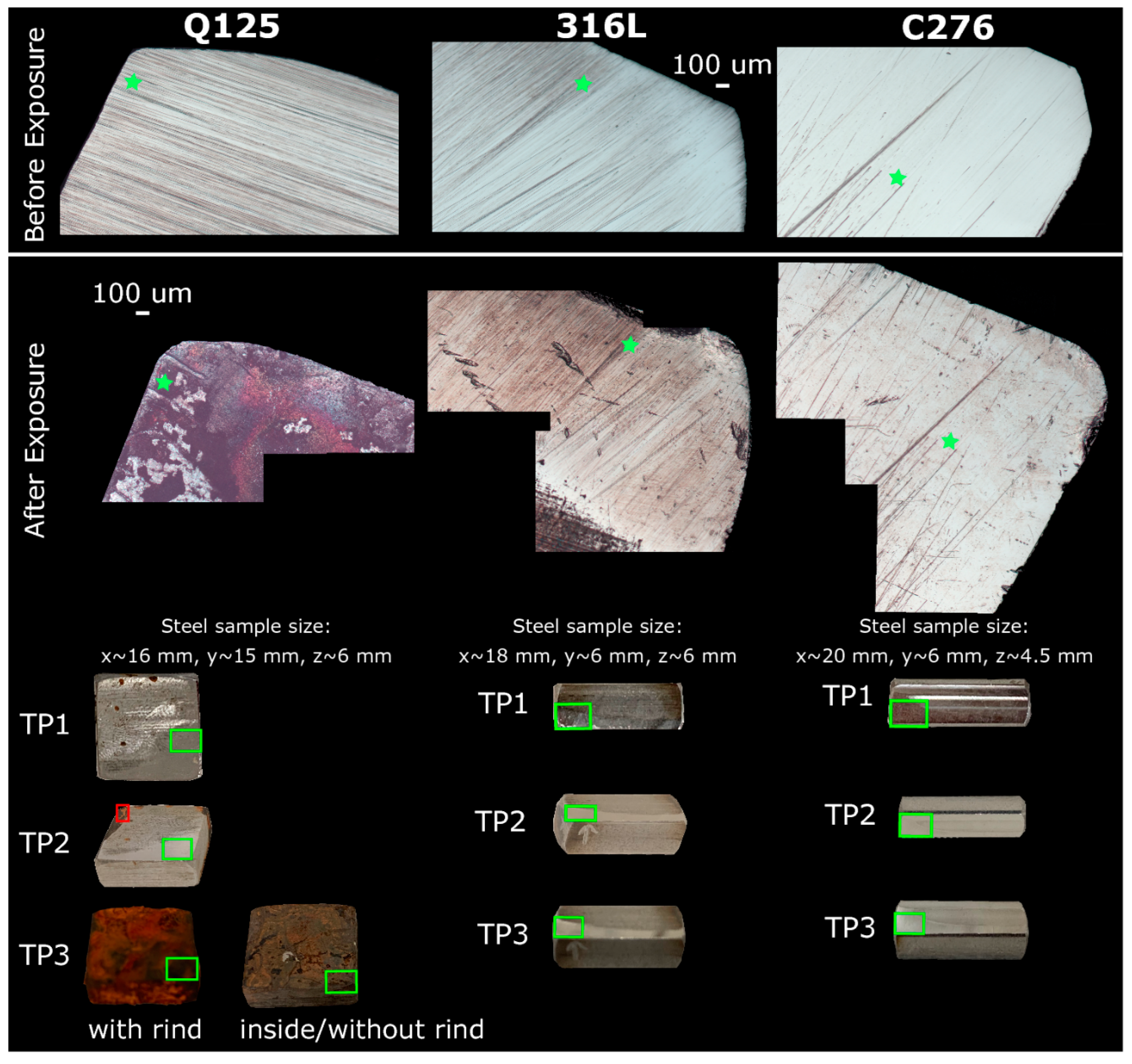
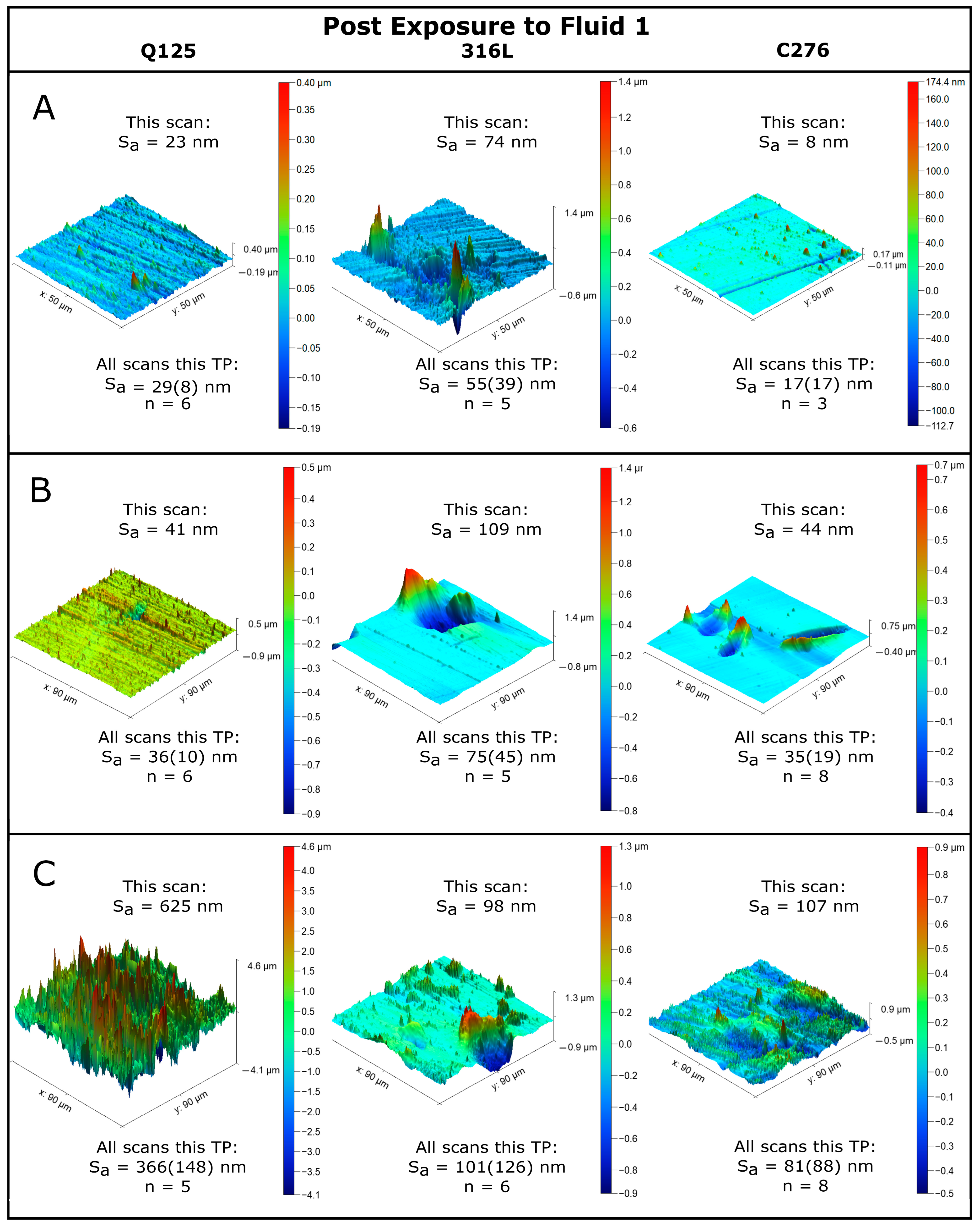
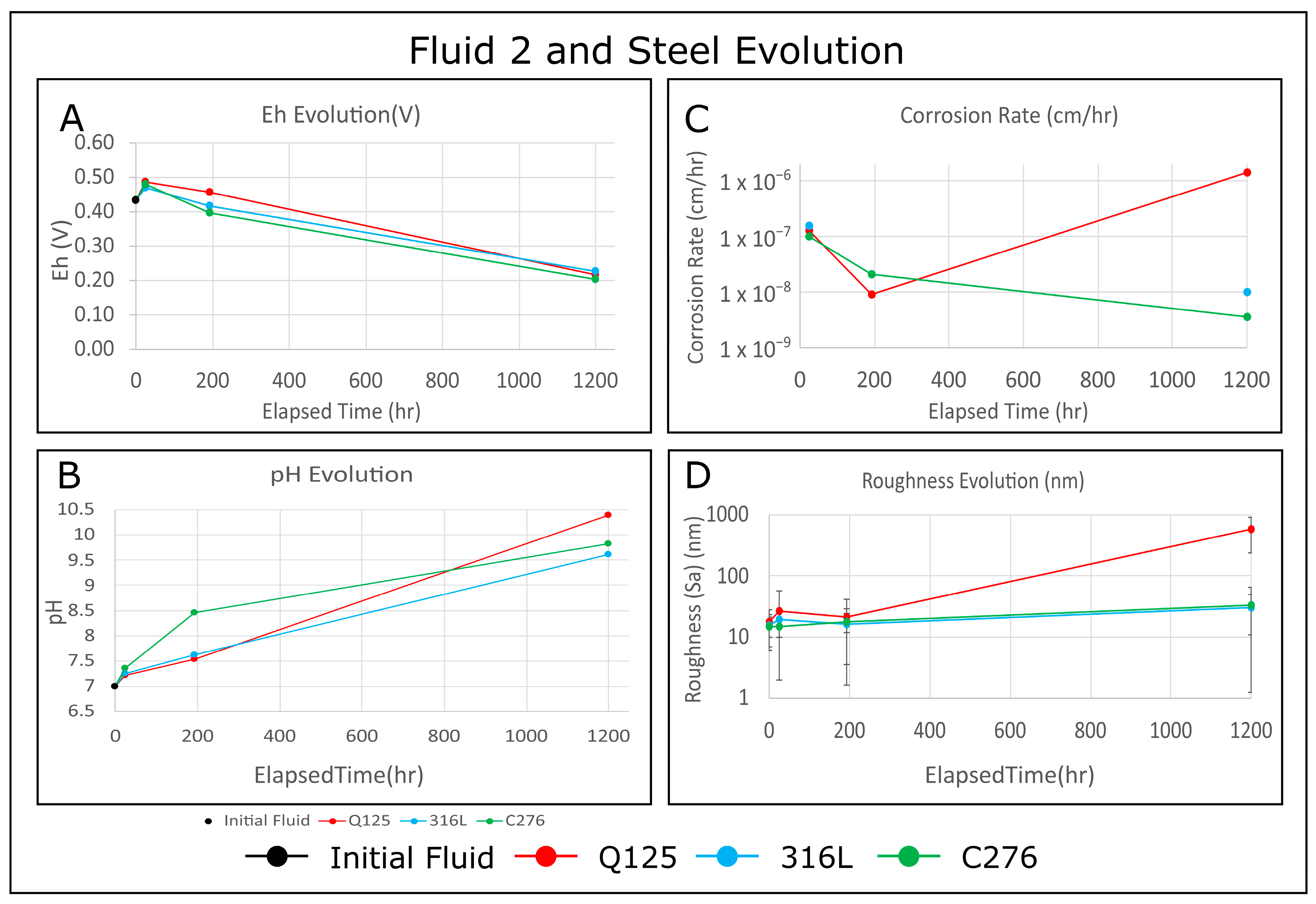
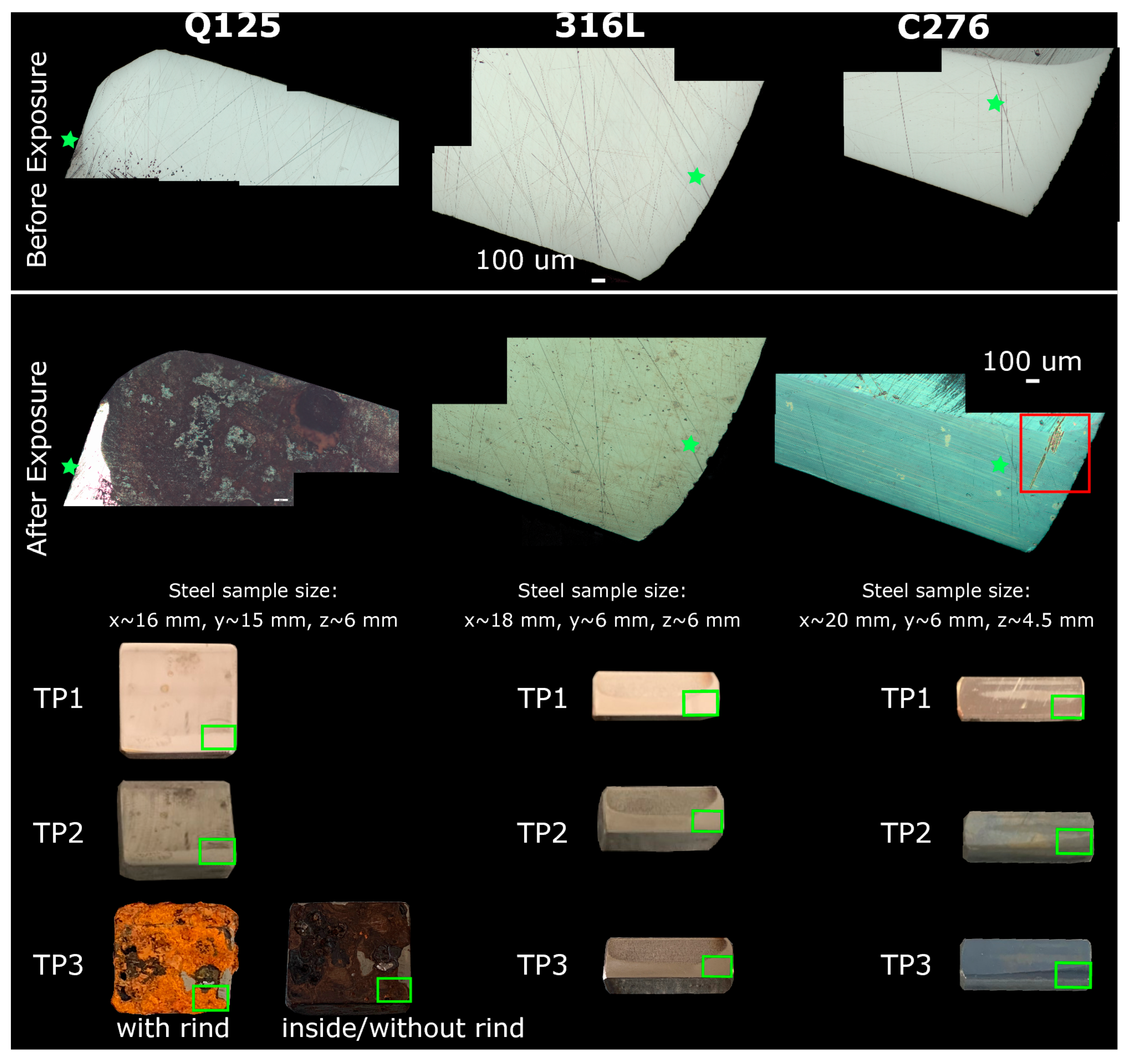
  • The AFM results show that Q125 performs approximately the same when exposed to both fluids and experiences general corrosion. After 1200 h of exposure, Q125, upon exposure to the reducing Fluid 1 solution, produced a weathering rind at a rate of 0.29% of the mass of the initial sample. Exposure to the oxidizing Fluid 2 solution produced a weathering rind at a rate of 0.74 wt % of the mass of the initial sample. Both the 316L and C276 steels performed similarly to each other, as both became progressively rougher over time when exposed to both corroding fluids. Pitting corrosion is the predominant form found on the surfaces of 316L and C276. The concentration of sulfur present in the fluids may be derived from steel dissolution. It is unknown if this is a contributing factor to the observed pitting corrosion or what the sulfur concentration (present as thiosulfate (e.g., [32])) must be for initiation. The pH and Eh of the initially reducing Fluid 1 change minimally after 1200 h, indicating that it is approaching atmospheric equilibrium at that point. Conversely, and perhaps perplexingly, after 1200 h, the pH of the initially oxidizing Fluid 2 evolves to become strongly basic and has a comparatively low Eh. This may be at least partially caused by H2O2 decay and the subsequent consumption of H+, followed by H2 production. Finally, our results have shown that significant steel corrosion can occur even after exposure to very low-ionic-strength (<0.0005 M) fluids.
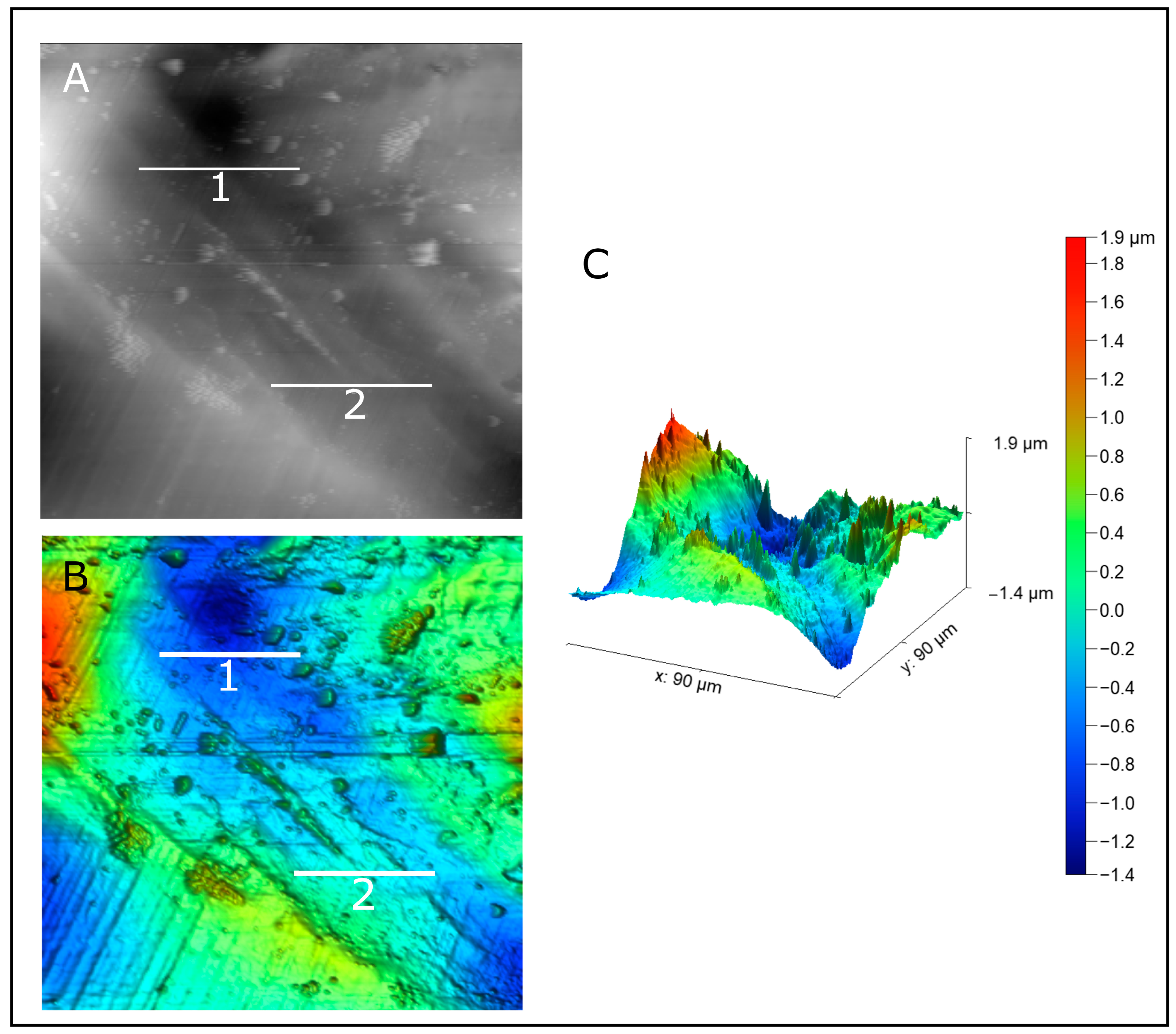
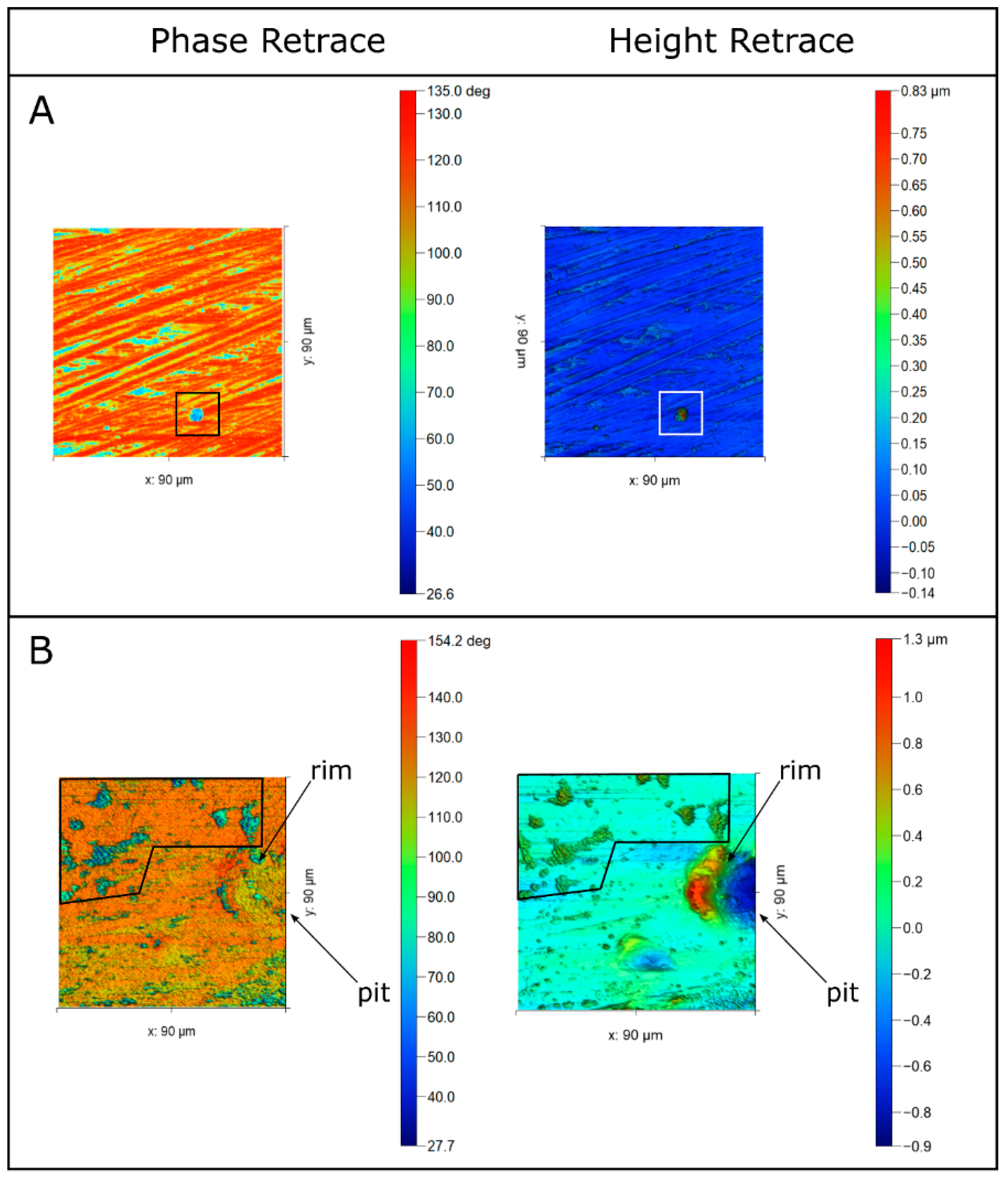
  • Redepositional peaks exhibit a significant spatial correlation with pitting corrosion, highlighting the utility of combining height retrace and phase retrace AFM maps. In qualitative terms, redepositional features are observed to have a lower phase retrace angle than the substrate’s bulk or approximate average angle. The accurate identification of these corrosion deposits could provide insights for selecting an appropriate antiscalant. AFM offers the advantage of providing ultra-high-resolution corrosion analysis.
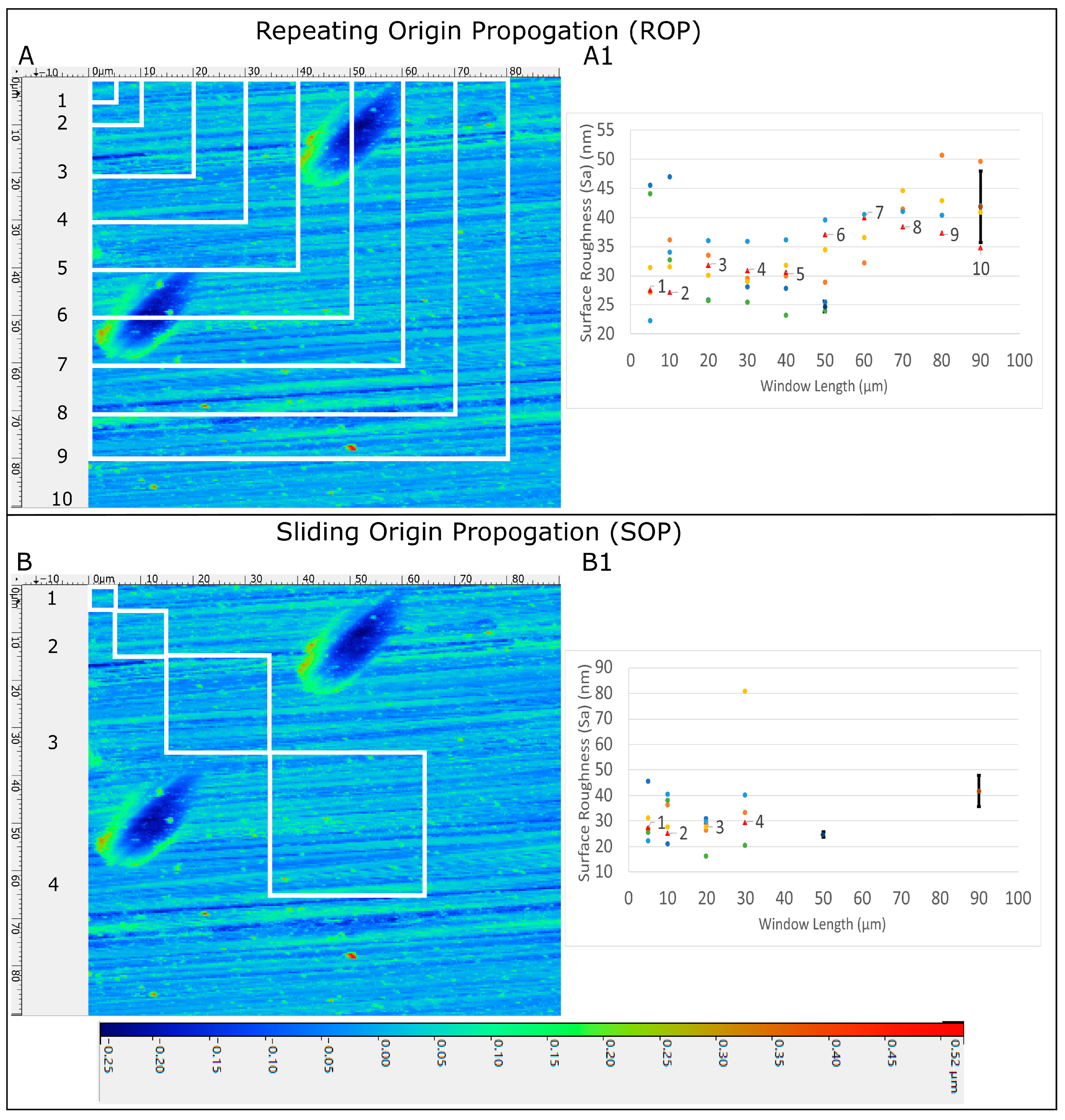
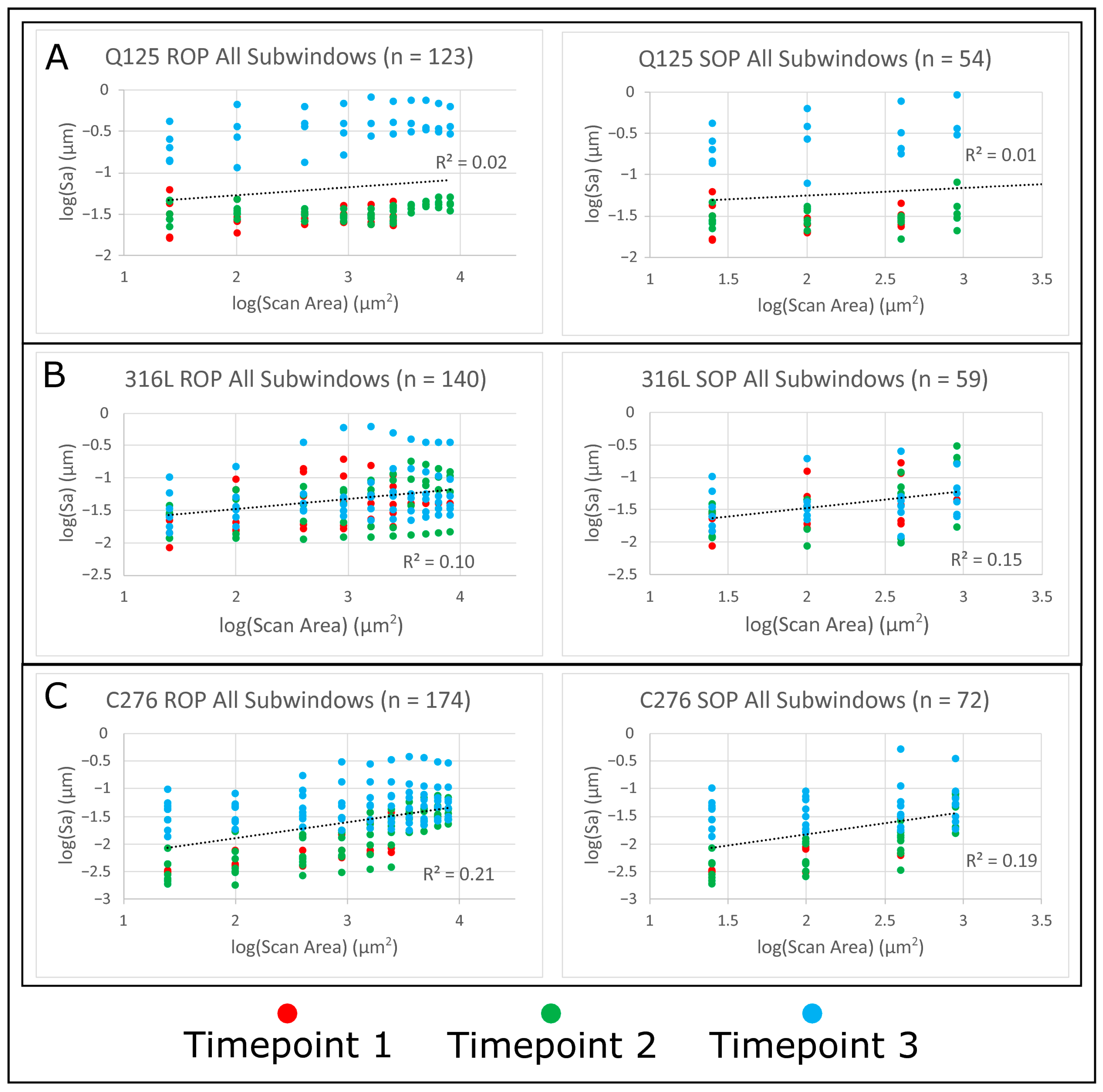
  • Although the surface features may appear heterogeneous, there seems to be no significant influence of sample site selection bias. Two models were created to examine the log–log relationship between the surface roughness and window scan area. Neither model exhibited a substantial correlation between these variables over approximately three log units, indicating a lack of scale sensitivity within this range. The specific spatial extent to which this observation no longer holds true remains unknown, and further research in this area will likely yield interesting results.

Author Contributions

Conceptualization, S.B., V.A. and S.S.; methodology, S.B., V.A. and S.S.; formal analysis, S.B.; investigation, S.B.; resources, S.S.; data curation, S.B.; writing—original draft preparation, S.B.; writing—review and editing, S.B., V.A. and S.S.; visualization, S.B.; supervision, V.A. and S.S.; project administration, S.S.; funding acquisition, S.S. All authors have read and agreed to the published version of the manuscript.

Funding

This work was funded by Department of Energy Office of Energy Efficiency & Renewable Energy (DOE EERE) Geothermal Technologies Program Award # DE-EE0009597 was awarded to to S. Sharma.

Data Availability Statement

The data presented in this study are available on request from the corresponding author.

Acknowledgments

We acknowledge the use of the WVU Shared Research Facilities, with special thanks to M. Redigolo and to Q. Wang. We wish to thank Northeast Natural Energy for the generous donation of the Q125 casing. We also thank C. Shobe for an insightful sliding window AFM discussion. Finally, we recognize the Department of Energy Office of Energy Efficiency and Renewable Energy (DOE EERE) Geothermal Technologies Program Award # DE-EE0009597 to S. Sharma, funding the research, as well as the authors’ time.

Conflicts of Interest

The authors declare no conflict of interest.

References

  1. Bäßler, R.; Burkert, A.; Saadat, A.; Kirchheiner, R.; Finke, M. Evaluation of Corrosion Resistance of Materials for Geothermal Applications; NACE-09377: Atlanta, Georgia, 2009. [Google Scholar]
  2. Faes, W.; Lecompte, S.; Van Bael, J.; Salenbien, R.; Bäßler, R.; Bellemans, I.; Cools, P.; De Geyter, N.; Morent, R.; Verbeken, K.; et al. Corrosion Behaviour of Different Steel Types in Artificial Geothermal Fluids. Geothermics 2019, 82, 182–189. [Google Scholar] [CrossRef]
  3. Liu, H.; Sun, J.; Qian, J.; Wang, B.; Shi, S.; Zhu, Y.; Wang, Y.; Neville, A.; Hua, Y. Revealing the Temperature Effects on the Corrosion Behaviour of 2205 Duplex Stainless Steel from Passivation to Activation in a CO2-Containing Geothermal Environment. Corros. Sci. 2021, 187, 109495. [Google Scholar] [CrossRef]
  4. Qi, W.; Gao, Q.; Zhao, Y.; Zhang, T.; Wang, F. Insight into the Stress Corrosion Cracking of HP-13Cr Stainless Steel in the Aggressive Geothermal Environment. Corros. Sci. 2021, 190, 109699. [Google Scholar] [CrossRef]
  5. Pound, B.G.; Abdurrahman, M.H.; Glucina, M.P.; Wright, G.A.; Sharp, R.M. The Corrosion of Carbon Steel and Stainless Steel in Simulated Geothermal Media. Aust. J. Chem. 1985, 38, 1133–1140. [Google Scholar] [CrossRef]
  6. Mundhenk, N.; Huttenloch, P.; Sanjuan, B.; Kohl, T.; Steger, H.; Zorn, R. Corrosion and Scaling as Interrelated Phenomena in an Operating Geothermal Power Plant. Corros. Sci. 2013, 70, 17–28. [Google Scholar] [CrossRef]
  7. Keserovic, A.; Bäßler, R. Geothermal Systems of Indonesia—Influence of Different Factors on the Corrosion Performance of Carbon Steel API Q125. In Proceedings of the World Geothermal Congress, Melbourne, Australia, 19–24 April 2015. [Google Scholar]
  8. Elgaddafi, R.; Ahmed, R.; Osisanya, S. Modeling and Experimental Study on the Effects of Temperature on the Corrosion of API Carbon Steel in CO2-Saturated Environment. J. Pet. Sci. Eng. 2021, 196, 107816. [Google Scholar] [CrossRef]
  9. Ropital, F.; Kittel, J. Corrosion Evaluation of Steels under Geothermal CO2 Supercritical Conditions. In Proceedings of the Proceedings World Geothermal Congress, Reykjavik, Iceland, 30 March–27 October 2021; p. 1. [Google Scholar]
  10. Han, J.; Carey, J.W.; Zhang, J. A Coupled Electrochemical–Geochemical Model of Corrosion for Mild Steel in High-Pressure CO2–Saline Environments. Int. J. Greenh. Gas Control 2011, 5, 777–787. [Google Scholar] [CrossRef]
  11. Zhao, M.-C.; Liu, M.; Song, G.-L.; Atrens, A. Influence of pH and Chloride Ion Concentration on the Corrosion of Mg Alloy ZE41. Corros. Sci. 2008, 50, 3168–3178. [Google Scholar]
  12. Lasebikan, B.A.; Akisanya, A.R.; Deans, W.F.; Macphee, D.E.; Boyle, L. The Effect of Ammonium Bisulfite on Sulfide in Brine/H2S Solution; OnePetro: Richardson, TX, USA, 2010. [Google Scholar]
  13. Rebak, R.B.; Yin, L.; Zhang, W.; Umretiya, R.V. Effect of the Redox Potential on the General Corrosion Behavior of Industrial Nuclear Alloys. J. Nucl. Mater. 2023, 576, 154257. [Google Scholar] [CrossRef]
  14. Saemundsson, K. Geothermal Systems in Global Perspective. In Short Course IV on Exploration for Geothermal Resources; UNU-GTP, KenGen and GDC: Naivasha, Kenya, 2009. [Google Scholar]
  15. Beckers, K.F.; Kolker, A.; Pauling, H.; McTigue, J.D.; Kesseli, D. Evaluating the Feasibility of Geothermal Deep Direct-Use in the United States. Energy Convers. Manag. 2021, 243, 114335. [Google Scholar]
  16. Weare, J.H.; Moller, N.; Greenberg, J.P. Modeling Geothermal Brine Process Chemistry. Geothermics 1986, 15, 401–405. [Google Scholar] [CrossRef]
  17. Maurice, V.; Marcus, P. Progress in Corrosion Science at Atomic and Nanometric Scales. Prog. Mater. Sci. 2018, 95, 132–171. [Google Scholar] [CrossRef]
  18. Bertrand, G.; Rocca, E.; Savall, C.; Rapin, C.; Labrune, J.-C.; Steinmetz, P. In-Situ Electrochemical Atomic Force Microscopy Studies of Aqueous Corrosion and Inhibition of Copper. J. Electroanal. Chem. 2000, 489, 38–45. [Google Scholar] [CrossRef]
  19. Martin, F.A.; Bataillon, C.; Cousty, J. In Situ AFM Detection of Pit Onset Location on a 304L Stainless Steel. Corros. Sci. 2008, 50, 84–92. [Google Scholar] [CrossRef]
  20. Nagarajan, S.; Rajendran, N. Crevice Corrosion Behaviour of Superaustenitic Stainless Steels: Dynamic Electrochemical Impedance Spectroscopy and Atomic Force Microscopy Studies. Corros. Sci. 2009, 51, 217–224. [Google Scholar] [CrossRef]
  21. Bai, P.; Zhao, H.; Zheng, S.; Chen, C. Initiation and Developmental Stages of Steel Corrosion in Wet H2S Environments. Corros. Sci. 2015, 93, 109–119. [Google Scholar] [CrossRef]
  22. Zhang, D.; Wang, M.M.; Jiang, N.; Liu, Y.; Yu, X.N.; Zhang, H.B. Electrochemical Corrosion Behavior of Ni-Doped ZnO Thin Film Coated on Low Carbon Steel Substrate in 3.5% NaCl Solution. Int. J. Electrochem. Sci. 2020, 15, 4117–4126. [Google Scholar] [CrossRef]
  23. Dirk, W.J.; Allen, C.A.; McAtee, R.E. Preliminary Evaluation of Materials for Fluidized Bed Technology in Geothermal Wells at Raft River, Idaho, and East Mesa, California. In Geothermal Scaling and Corrosion; Casper, L.A., Pinchback, T.R., Eds.; ASTM STP 717: West Conshohocken, PA, USA, 1980; pp. 69–80. [Google Scholar]
  24. Tardiff, G.E.; Snell, E.O. Failure Analysis of a Hastelloy C-276 Geothermal Injection Pump Shaft; Lawrence Livermore Laboratory: Livermore, CA, USA, 1979.
  25. Phair, K. 11—Direct Steam Geothermal Energy Conversion Systems: Dry Steam and Superheated Steam Plants. In Geothermal Power Generation; Di Pippo, R., Ed.; Woodhead Publishing: Cambridge, UK, 2016; pp. 291–319. [Google Scholar] [CrossRef]
  26. Morana, R.; Nice, P.I. Corrosion Assessment of High Strength Carbon Steel Grades P-110, Q-125, 140 and 150 for H2S Containing Producing Well Environments; OnePetro: Richardson, TX, USA, 2009. [Google Scholar]
  27. Jeon, J.; Ahmed, R.; Elgaddafi, R.; Teodoriu, C. Hydrogen Embrittlement of High-Strength API Carbon Steels in H2S and CO2 Containing Environments. J. Nat. Gas Sci. Eng. 2022, 104, 104676. [Google Scholar] [CrossRef]
  28. Grgur, B.N.; Trišović, T.L.; Rafailović, L. Corrosion of Stainless Steel 316Ti Tank for the Transport 12–15% of Hypochlorite Solution. Eng. Fail. Anal. 2020, 116, 104768. [Google Scholar] [CrossRef]
  29. Snyder, D.M.; Beckers, K.F.; Young, K.R.; Johnston, B. Analysis of Geothermal Reservoir and Well Operational Conditions Using Monthly Production Reports from Nevada and California. GRC Trans. 2017, 41, 2844–2856. [Google Scholar]
  30. Kamila, Z.; Kaya, E.; Zarrouk, S.J. Reinjection in Geothermal Fields: An Updated Worldwide Review 2020. Geothermics 2021, 89, 101970. [Google Scholar] [CrossRef]
  31. Kanoglu, M. Exergy Analysis of a Dual-Level Binary Geothermal Power Plant. Geothermics 2002, 31, 709–724. [Google Scholar] [CrossRef]
  32. Akpanyung, K.V.; Loto, R.T. Pitting Corrosion Evaluation: A Review. J. Phys. Conf. Ser. 2019, 1378, 022088. [Google Scholar] [CrossRef]
  33. Hoeckelman, R.F. Optical Properties of Chromium-Plated Steel. J. Electrochem. Soc. 1972, 119, 1310. [Google Scholar] [CrossRef]
  34. He, L.-F.; Roman, P.; Leng, B.; Sridharan, K.; Anderson, M.; Allen, T.R. Corrosion Behavior of an Alumina Forming Austenitic Steel Exposed to Supercritical Carbon Dioxide. Corros. Sci. 2014, 82, 67–76. [Google Scholar] [CrossRef]
  35. Bagotsky, V.S. Fundamentals of Electrochemistry, 2nd ed.; The Electrochemical Society Series; Wiley: Hoboken, NJ, USA, 2006. [Google Scholar]
  36. Chilingar, G.V.; Mourhatch, R.; Al-Qahtani, G.D. The Fundamentals of Corrosion and Scaling for Petroleum & Environmental Engineers; Gulf Oublishing Company: Houston, TX, USA, 2013. [Google Scholar]
  37. Dubois, F.; Mendibide, C.; Pagnier, T.; Perrard, F.; Duret, C. Raman Mapping of Corrosion Products Formed onto Spring Steels during Salt Spray Experiments. A Correlation between the Scale Composition and the Corrosion Resistance. Corros. Sci. 2008, 50, 3401–3409. [Google Scholar] [CrossRef]
  38. Vu, T.N.; Volovitch, P.; Ogle, K. The Effect of pH on the Selective Dissolution of Zn and Al from Zn–Al Coatings on Steel. Corros. Sci. 2013, 67, 42–49. [Google Scholar] [CrossRef]
Figure 1. Fluid 1 evolution and steel behavior from each Wheaton bottle containing a single piece of steel. (A,B) Fluid evolution. (C,D) Steel roughness and corrosion rate. The surface roughness values are averages of the entire ROI scan area and are taken from the Fluid 1 AFM data in Table 2. Surface roughness uncertainties are at the 1 σ level.
Cmd 04 00030 g001
Figure 2. Example of probable polishing relic from 316L TP3 from Fluid 1. Red areas represent topographic highs and blue areas represent topographic lows. (A) The transects 1 and 2 are both 30 µm in length. This is the diameter of the first diamond lapping film used in sample polishing. (B) Colorized version of the same ROI. (C) Oblique view with scale bar. Note the correlation between the transects and the deep linear valley, interpreted as a relic from the 30 µm diamond lapping film.
Cmd 04 00030 g002
Figure 3. Images of the selected region for AFM analysis on each steel sample before and after the full 1200 h exposure to Fluid 1. The “after exposure” samples are multiple images photomerged at the same magnification as the single “before exposure” image. The green stars refer to polishing relics. Green rectangles indicate the general ROI that was analyzed using AFM. Examples of AFM topographic maps from these areas are presented in Figure 4. The red rectangle on Q125 from TP2 is an unpolished area and corresponds to the “u.p.” data row in Fluid 1 of Table 2. Photographs except for Q125 from TP3 illustrate both an oxidized rind and the inside of the same sample after rind removal. This is the surface used for AFM analysis (Figure 4, Table 2). The interior surface is the surface that was analyzed using AFM.
Cmd 04 00030 g003
Figure 4. AFM height retrace topographic maps at each timepoint after exposure to Fluid 1. Red areas represent topographic highs and blue areas represent topographic lows. Note that the text below the AFM graphic is the average of each ROI for that piece of steel at the corresponding timepoint. Values at the 1σ level are given in parentheses. All AFM maps are shown using the same amount of scale exaggeration unless otherwise noted. (A) TP1. (B) TP2. (C) TP3. The scale exaggeration for the Q125 AFM topographic map has been reduced by a factor of 1.9 to reduce noise.
Cmd 04 00030 g004
Figure 5. Fluid 2 evolution and steel behavior from each Wheaton bottle containing a single piece of steel. (A,B) Fluid evolution. (C,D) Steel roughness and corrosion rate. Note that, for example, 1E-07 cm/hr is equivalent to 1 × 10⁻⁷ cm/hr. The surface roughness values are averages of the entire ROI scan area. The surface roughness values are averages of the entire ROI scan area and are taken from the AFM Fluid 2 data in Table 2. Surface roughness uncertainties are at the 1 σ level.
Cmd 04 00030 g005
Figure 6. Photomerge images of the selected region for AFM analysis on each steel sample before and after the entire 1200 h exposure to Fluid 2. Both “before exposure” and “after exposure” images were taken at the same level of magnification. The green stars refer to polishing relics. Green rectangles indicate the general ROI that was analyzed using AFM (Figure 7). The red rectangle is a specific location referenced in the text and the corresponding AFM map is found in Figure 7C. Photographs except for Q125 from TP3 illustrate an oxidized rind and the inside of the same sample after rind removal.
Cmd 04 00030 g006
Figure 7. AFM height retrace topographic maps at each timepoint after exposure to Fluid 2. Red areas represent topographic highs and blue areas represent topographic lows. Note that the text below the AFM graphic is the average of each ROI for that piece of steel at the corresponding timepoint. Values at the 1σ level are given in parentheses. All images are shown using the same amount of scale exaggeration unless otherwise noted. (A) TP1. (B) TP2. (C) TP3. Regarding Q125, the scale exaggeration for this AFM topographic map has been reduced by a factor of 1.9 to reduce noise. The red box outlining the C276 AFM map corresponds to the same ROI outlined in Figure 6.
Cmd 04 00030 g007
Figure 8. Redepositional features on steel surfaces. (A) Spire structure on C276 steel after TP3-ROI, outlined with a box. (B) Pitting corrosion pit with immediately adjacent redepositional rim on 316L TP3. Amorphous elevated structures are highly spatially correlated with phase retrace—ROI outlined in black.
Cmd 04 00030 g008
Figure 9. AFM topographic maps from Q125 TP2 after exposure to Fluid 1 (n = 6) comparing the surface roughness values obtained from the ROP and SOP window models. The spatial resolution is within 0.2 μm of the reported coordinates. (A) ROP results with ten square sub-windows within the full 90 × 90 μm window. (B) SOP results with four square sub-windows within the full 90 × 90 μm window. (A1,B1) Surface roughness obtained from each sub-window (numbered datapoints denoted by red triangles correspond to the respective sub-window in (A,B)). The remaining datapoints denoted by circles are the surface roughness values from additional AFM topographic maps of Q125 from TP2 after exposure to the low-Eh fluid. The black bar represents the 1σ of the full maps at the 50 × 50 μm scale (n = 2) and the 90 × 90 μm scale (n = 4), and is centered about the mean.
Cmd 04 00030 g009
Figure 10. Log–log analysis of scan area window size versus surface roughness for both ROP and SOP models. All data are AFM results obtained after exposure to Fluid 1. Each trendline pertains to all datapoints (independent of time). (A) Q125 steel. (B) 316L steel. (C) C276 steel.
Cmd 04 00030 g010
Table 1. Steel composition, industrial application, and calculated molar mass and ionic charge. The C276 and 316L elemental wt % are given by the manufacturer, and the values for Q125 are the maximum elemental wt % given by the sample donor. Dirk et al., 1980 [23]; Tardiff and Snell, 1979 [24]; Phair, 2016 [25]; Morana and Nice, 2009 [26]; Jeon et al., 2022 [27]. The ionic charge is calculated using oxidation states of 4, 2, 2, 1, 2, 2, 6, −3, 2, −3, −2, 4, 2, and 6 for C to W, respectively.
Steel Name AISI/EN/APIPurpose/UseElemental wt %M
g/mol
Ionic Charge
CCoCrCuFeMnMoNNiPSSiVW
C276/2.4819/-Heat exchangers [23] and pump shafts [24]0.0060.0115.60.025.70.5216.2-580.0030.0010.050.013.6767.92.8
316L/1.4404/-Condensers [25] and heat exchangers [23]0.02-16.70.5568.51.672.030.0533 10.10.0270.027 20.4--56.22.1
-/-/Q125High strength/pressure casing [26,27]0.35-1.5-94.91.350.85-0.990.020.01---56.02.0
Table 2. Corrosion rates and AFM results for each fluid and grade of steel at each timepoint. All steel data are taken from ROIs within the polished locations on each steel corner, while the unpolished (u.p.) Q125 AFM data pertain to an ROI at TP2.
At TP0:
pH = 7
T = 75 °C
TP0TP1TP2TP3
Time: 0 hTime: 24 h, Elapsed Time: 24 hTime: 168 h, Elapsed Time: 192 hTime: 1008 h, Elapsed Time: 1200 h
Average Surface Rough. 1σ (nm)Average Trans.
1σ (nm)
Average Surface Rough.
1σ (nm)
Average Trans.
1σ (nm)
Corr. Rate (mm/y)Average Surface Rough.
1σ (nm)
Average Trans.
1σ (nm)
Corr. Rate (mm/y)Average Surface Rough. 1σ (nm)Average Trans.
1σ (nm)
Corr. Rate (mm/y)
Standard Deviations are Reported at the 1σ Level and Pertain Values Inside Parentheses
Fluid 1Q12530 (4)400 (43)29 (8)510 (159)8.2 × 10−336 (10)972 (301)0.051366 (148)6286 (2428)0.11
Q125 (u.p.)1351649---~1352>15,197----
316L17 (32)415 (282)55 (39)1296 (746)8.8 × 10−375 (44)1204 (833)<LOD101 (126)1824 (901)<LOD
C27623 (15)617 (160)17 (17)424 (370)<LOD34 (19)1003 (435)<LOD81 (88)1477 (1092)<LOD
Fluid 2Q12517 (11)748 (312)27 (30)1003 (523)1.1 × 10−221 (20)652 (593)8.1 × 10−4582 (338)6864 (2724)0.13
316L15 (6)466 (84)20 (10)562 (239)1.8 × 10−216 (13)687 (397)<LOD30 (20)696 (369)8.6 × 10⁻⁴
C27615 (8)337 (216)15 (13)475 (255)8.7 × 10−318 (6)508 (120)1.8 × 10−333 (32)1085 (1521)3.1 × 10⁻⁴
Table 3. Log–log surface roughness analysis of Q125 steel after exposure to Fluid 1 for all timepoints for both ROP and SOP models.
Log–Log Analysis after Fluid 1 ExposureROP Range log(Sa) (µm)ROP Range log(Scan Area) (µm2)SOP Range log(Sa) (µm)SOP Range log(Scan Area) (µm2)
Q125 TP10.5812.0000.5811.204
Q125 TP20.3582.5110.6921.556
Q125 TP30.8522.5111.0671.556
316L TP11.3692.5111.2881.556
316L TP21.1962.5111.5461.556
316L TP31.6342.5111.3281.556
C276 TP11.0802.0000.9611.204
C276 TP21.6192.5111.6391.556
C276 TP31.4542.5111.5771.556
Disclaimer/Publisher’s Note: The statements, opinions and data contained in all publications are solely those of the individual author(s) and contributor(s) and not of MDPI and/or the editor(s). MDPI and/or the editor(s) disclaim responsibility for any injury to people or property resulting from any ideas, methods, instructions or products referred to in the content.

