Article

Sex Differential Dynamics in Coherent Mortality Models

by
Snorre Jallbjørn
1,2 and
Søren Fiig Jarner
1,*
1
Department of Mathematical Science, University of Copenhagen, 2100 Copenhagen, Denmark
2
Danish Labour Market Supplementary Pension Fund, Kongens Vænge 8, 3400 Hillerød, Denmark
*
Author to whom correspondence should be addressed.
Forecasting 2022, 4(4), 819-844; https://doi.org/10.3390/forecast4040045
Submission received: 12 August 2022 / Revised: 23 September 2022 / Accepted: 27 September 2022 / Published: 29 September 2022
(This article belongs to the Special Issue Mortality Modeling and Forecasting)

Abstract

:
The main purpose of coherent mortality models is to produce plausible, joint forecasts for related populations avoiding, e.g., crossing or diverging mortality trajectories; however, the coherence assumption is very restrictive and it enforces trends that may be at odds with data. In this paper we focus on coherent, two-sex mortality models and we prove, under suitable conditions, that the coherence assumption implies sex gap unimodality, i.e., we prove that the difference in life expectancy between women and men will first increase and then decrease. Moreover, we demonstrate that, in the model, the sex gap typically peaks when female life expectancy is between 30 to 50 years. This explains why coherent mortality models predict narrowing sex gaps for essentially all Western European countries and all jump-off years since the 1950s, despite the fact that the actual sex gap was widening until the 1980s. In light of these findings, we discuss the current role of coherence as the gold standard for multi-population mortality models.

1. Introduction

The aim of coherent multi-population mortality models is to forecast the mortality of related populations preserving the structural differences observed in the past, e.g., preserving differences between countries, regional differences within a country, or higher mortality for men than for women. The idea is to prevent divergence or implausible crossings of mortality trajectories that can arise from forecasting each population individually. The concept of coherence was introduced by Li and Lee [1], as an extension to the popular Lee-Carter model [2], and later formalized by Hyndman et al. [3]. Since then a number of coherent models have been proposed, both within the Lee–Carter framework [4,5,6,7], with added cohort effects [8,9,10], and based on the functional data approach [3,11]. Today, coherence still serves as the gold standard for multi-population mortality models.
Technically, coherence means that the ratio of age-specific mortality rates of the populations being forecasted converges (to finite, age-specific constants). This requirement ties the forecasts together and it ensures that differences in aggregate characteristics, e.g., survival probabilities and life expectancies, remain bounded as desired. The flip-side, however, is that converging mortality sex ratios may not be supported by data and enforcing it can lead to unrealistic continuations of historic trends despite the intention, see [12,13]. In this paper, we investigate and exemplify the implications of coherence in two-sex mortality models, in particular, the implications for the dynamics of the life expectancy difference between the sexes.
The sex differential in life expectancy is a key statistic for summarizing and communicating discrepancies in sex-specific mortality curves. The differential has varied considerably over time, although its general shape has been fairly consistent from country to country. In the Western world, the gap has the shape of a (unimodal) hill; the differential widened substantially in favor of women throughout most of the 20th century, but the trend reversed around the 1980s and the gap has continued to narrow since then [14,15].
Studies have sought to explain the observed trends in the sex gap through changes in behavioral, socioeconomic, and health factors, for example, smoking and drinking habits [16,17,18], labor market participation [19,20], risk behavior [21], and cause-of-death contributions [22,23,24]. The rationale being that changes in external risk factors explain changes in mortality sex ratios, which in turn explain trends in the life expectancy differential. This common-sense reasoning assumes that changing mortality sex ratios is the main driver of the sex gap, both when it increases and when it decreases. However, demographic analyses have challenged this assumption. In particular, Glei and Horiuchi [15] and Cui et al. [25] show that while the widening sex gap was indeed caused by changing mortality sex ratios, the narrowing of the sex gap was primarily caused by general mortality improvements for both sexes in combination with heterogeneity in the death distributions. In simpler terms, the expanding sex gap in the Western world was caused primarily by female mortality improving faster than male mortality (i.e., changing mortality sex ratios), while the subsequent narrowing of the gap was caused primarily by improvements in mortality for both sexes, with women retaining their relative advantage (i.e., improvements under stable mortality sex ratios).
In this paper, we demonstrate that coherent two-sex models generally imply unimodal sex gap dynamics. At first sight, this might seem as an attractive feature given that the sex gap in the Western world has also been unimodal, as described above. It turns out, however, that in practice the forecasts are almost always on the declining part of the sex gap trajectory. This in turn implies that coherent models are ill-suited to forecast the mortality in periods with increasing sex gaps. Coincidentally, the concept of coherence was introduced after a prolonged period of narrowing sex gaps and the continuation of this trend was seen as an argument in favor of coherent models, see Hyndman et al. [3]. That coherent models produce sensible forecasts only in periods with narrowing sex gaps does however question the status of coherence as a universally desirable feature in multi-population models. We will return to this point towards the end of the paper.
The rest of the paper is organized as follows. First, we illustrate the evolution of the sex gap in Western Europe since the 1950s and we survey the existing sex gap decomposition methods, formalizing the ratio and level effects responsible for the widening and the narrowing of the gap respectively. Second, we present our main mathematical result showing sex gap unimodality in (strongly) coherent models under certain conditions; we discuss the intuition behind the conditions and show by example when multi-modality can occur. Third, we analyze a dynamic Gompertz model as a simple example of a coherent model satisfying the conditions; we compute the typical sex gap trajectories that can arise under this model and we use this to explain why the forecasted sex gap will almost always be narrowing. Fourth, we apply the coherent models of Li and Lee [1] and Hyndman et al. [3] to Western European countries at selected jump-off years during the period with expanding sex gaps; with reference to the mathematical results, we discuss why the majority of these forecasts predict narrowing gaps. Finally, we end with some concluding remarks.

Data and Notation

Data is obtained from the Human Mortality Database [26] and consists of death counts, D ( x , t ) , and central exposure-to-risk estimates, E ( x , t ) , on Lexis A-sets, that is, age-period cells of the form [ x , x + 1 ) × [ t , t + 1 ) for integer ages x { 0 , , 110 } and calendar years t { 1950 , , 2020 } for countries in Western Europe. The empirical death rate is estimated as
m ( x , t ) = D ( x , t ) / E ( x , t ) .
Death rates for Western Europe are obtained by pooling death and exposure counts across individual countries. Throughout, (period) life expectancies are calculated by numerical integration whenever a continuous mortality curve is available, and under the assumption of piecewise constant mortality, whenever the mortality curve is only available at integer ages. That is,
e ( x , t ) = 1 S ( x , t ) x ω S ( y , t ) d y = x ω e x y μ ( z , t ) d z d y = i = x ω 1 1 e μ ( i , t ) μ ( i , t ) e j = x i 1 μ ( j , t ) ,
where S ( x , t ) = exp ( 0 x μ ( y , t ) d y ) is the (period) survival function, μ ( x , t ) the force of mortality at age x and time t, and  ω ( 0 , ) the age at truncation. Note that ω is not necessarily the maximum attainable age, and we do not assume that μ ( x ) = for x > ω . We return to the role of the truncation age later in the paper. The last equality in Equation (2) assumes piecewise constant mortality, a full derivation is given in Appendix C.

2. Changes in Mortality, Life Expectancy, and Sex Differentials

In this section, we briefly survey the existing methods for decomposing changes in life expectancy and the sex differential. This provides the basis for the subsequent treatment of sex differentials in coherent mortality models.

2.1. Decomposing Changes in Life Expectancy

There are two main approaches for decomposing changes in life expectancy into constituent parts. The first approach, pioneered by Pollard [27] and Arriaga [28], focuses on the effect of changing mortality from one age-specific schedule to another, and is typically used to assess how different age groups contribute in driving life expectancy progress between two distinct points in time. The second approach, popularized by Keyfitz [29], examines the effect of a local change to the mortality curve by quantifying how various age-specific improvements in mortality,
ρ ( x , t ) : = μ ˙ ( x , t ) μ ( x , t ) = t log μ ( x , t ) ,
translate into changes in life expectancy. In (3) and throughout, a dot over a function is used to denote its derivative with respect to time as in Vaupel and Romo [30].
Analyzing the effects of local change have been instrumental for understanding the linkage between the age pattern of mortality and the trends in e ( 0 , t ) observed in data. Indeed, studies have shown that the dispersion of the life table death distribution is a main determinant of the pace at which life expectancy improves [29,31,32].
The average number of life-years lost due to death (lifespan disparity) is given by
e ( t ) = 0 ω w ( x , t ) d x ,
where w ( x , t ) = μ ( x , t ) S ( x , t ) e ( x , t ) is the (life table) probability of dying at age x times the remaining life expectancy at that age. Lifespan disparity, e , is a dispersion measure, i.e., it quantifies the effect of age of death being distributed across ages. At one extreme, if  e is zero then everyone dies at the same age. Conversely, if  e is large then the population experiences a high number of premature deaths and large gains in e ( 0 , t ) can be made by reducing mortality. Improvements among the young are particularly important as more life years are lost upon death at these ages. This relation was formalized by Keyfitz [29] who showed that if the same rate of mortality improvement, ρ ( t ) , applies to all ages, then the change in life expectancy can be expressed as e ˙ ( 0 , t ) = ρ ( t ) e ( t ) . The absolute change in e ( 0 , t ) can thus be interpreted as a product of the proportion of deaths averted ( ρ ) and the average number of life-years gained ( e ) by those who now survive.
Vaupel and Romo [30] generalized Keyfitz’s formula to the case of age-dependent improvement rates, and suggested that a change in life expectancy at birth be decomposed into two components  
e ˙ ( 0 , t ) = 0 ω ρ ( x , t ) w ( x , t ) d x = ρ ¯ ( t ) e ( t ) + Cov ( ρ , e ) ,
where the first term captures the main effect of improvement, while the second term arises due to heterogeneity in ρ ( x , t ) at different ages. In (5), ρ ¯ denotes the average rate of improvement and Cov ( ρ , e ) is the covariance between improvement rates and life expectancy, see Vaupel and Romo [30] for details. Equation (5) is often taken as the basis for deriving the dynamics of life expectancy sex differentials.

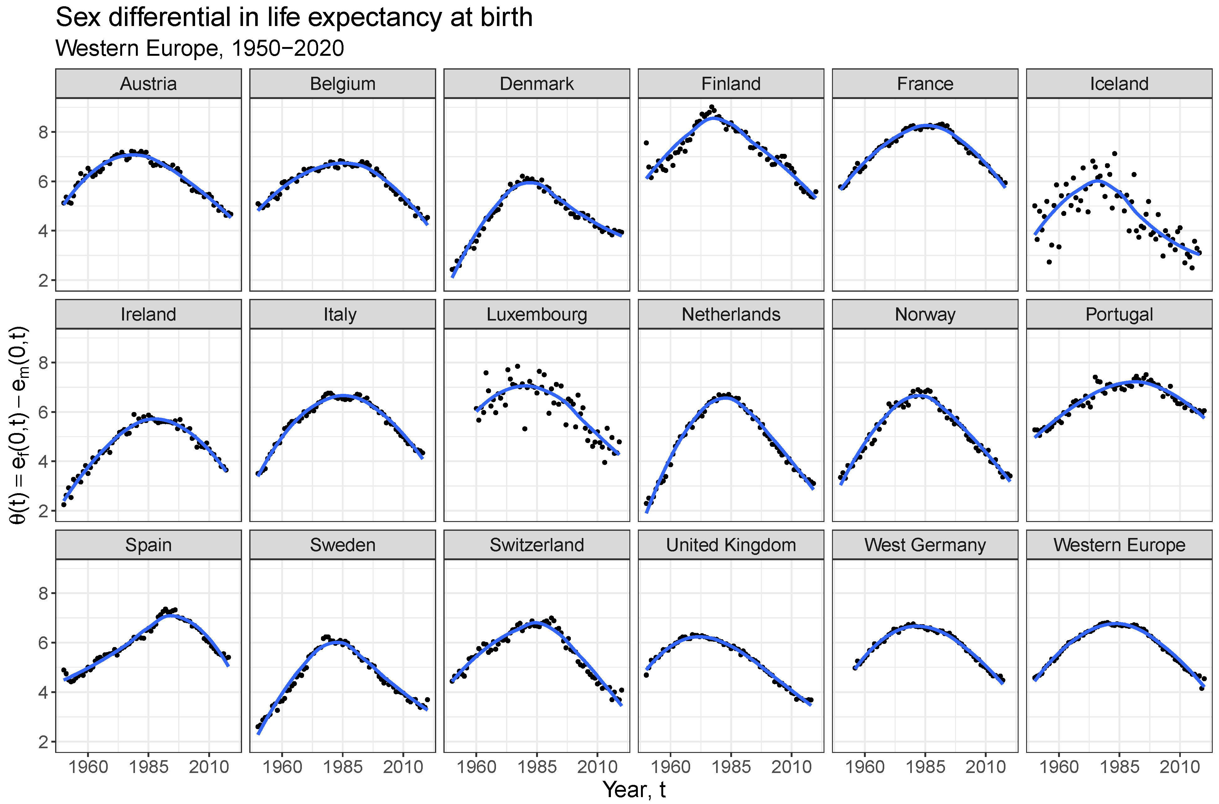
2.2. The Rise and Fall of Sex Differentials in Western Europe

The difference in life expectancy at birth between females and males in a given population (the sex gap) is defined as
θ ( t ) = e f ( 0 , t ) e m ( 0 , t ) = 0 ω e 0 x μ f ( y , t ) d y d x 0 ω e 0 x μ m ( y , t ) d y d x ,
where the subscripts f and m denote female and male quantities, respectively. In applications we might be interested also in (remaining) life expectancy and sex differential at other ages than 0; all formulas apply, mutatis mutandis, for a general age, but for ease of notation we develop the theory for age 0 only.
Figure 1 shows the evolution of the sex gap over time since 1950 in Western Europe. The overall pattern is the same across all countries with the gap being shaped as a countryside hill. That is, the gap initially widened, but has since fallen into a decline with differentials currently around 3–6 years. The timing of the turning point varies by country, occurring first in the United Kingdom circa 1970 and lastly in Spain towards the end of the 1990s.
The rise and fall of sex differentials observed in the data has recently been studied using demographic decompositions. The principal method of Glei and Horiuchi [15] separates change in θ into effects due to changing mortality ratios and effects due to changing mortality levels, namely  
θ ˙ ( t ) = 0 ω w m ( x , t ) + w f ( x , t ) 2 c ˙ ( x , t ) c ( x , t ) d x + 0 ω [ w m ( x , t ) w f ( x , t ) ] ζ ˙ ( x , t ) ζ ( x , t ) d x ,
where c ( x , t ) = μ m ( x , t ) / μ f ( x , t ) is the mortality sex ratio, ζ ( x , t ) = μ m ( x , t ) μ f ( x , t ) the geometric average of the two mortality rates, and, w f and w m are as in Equation (4) for females and males, respectively. Note that c ˙ ( x , t ) / c ( x , t ) = t log c ( x , t ) = ρ f ( x , t ) ρ m ( x , t ) , and  ζ ˙ ( x , t ) / ζ ( x , t ) = t log ζ ( x , t ) = [ ρ f ( x , t ) + ρ m ( x , t ) ] / 2 . It follows that the ratio effect is positive when ρ f > ρ m , while the sign of the level effect depends on the relative size of mortality dispersion for the two sexes (as measured by w f and w m ); thus, the two effects can work either in the same direction, or against each other.
Using (7), Glei and Horiuchi [15] show that the initial widening of θ seen in Figure 1 is caused primarily by women experiencing comparatively larger rates of mortality improvements than men ( ρ f > ρ m ), while the subsequent narrowing is largely attributable to differential dispersion between the sexes ( w m > w f ) in combination with general improvements. These results are echoed by Cui et al. [25], who use (5) to separate θ ˙ into three components of change through which they obtain conditions for the sex gap to be widening, narrowing, or at a turning point.

Pollard’s Paradox

Glei and Horiuchi [15] and Cui et al. [25] both stress that differential dispersion plays a pivotal role in determining changes in θ . In fact, differential dispersion may give rise to somewhat counter-intuitive changes. Pollard [27], for example, demonstrated that two populations may experience the same absolute change in mortality, but, at the same time, a widening life expectancy differential. The argument is as follows. For  i { f , m } , consider an absolute decrease in mortality at all ages, that is, μ ˜ i ( x ) = μ i ( x ) ε for some ε > 0 . Let S ˜ i ( x ) = S i ( x ) e ε x denote the new probability of surviving to age x. Assuming μ f ( x ) < μ m ( x ) for all x, the new life expectancy differential is then larger than before,
θ = 0 ω S f ( x ) S m ( x ) d x < 0 ω S f ( x ) S m ( x ) e ε x d x = θ ( ε , ε ) ,
where θ ( ε f , ε m ) denotes the life expectancy differential when female mortality is decreased by ε f and male mortality by ε m . If we subsequently increase female mortality slightly, we obtain a situation with 0 < ε f < ε and θ < θ ( ε f , ε ) , i.e., a narrowing mortality differential with a widening life expectancy differential. This phenomenon is sometimes referred to as Pollard’s paradox.
In a similar fashion we can argue that a narrowing life expectancy differential does not guarantee narrowing mortality ratios. For instance, taking outset in Keyfitz’s formula, when the rate of improvement is the same at all ages, we have
θ ˙ ( t ) = ρ f ( t ) e f ( t ) ρ m ( t ) e m ( t ) .
Suppose e m ( t ) > e f ( t ) , and let k = e m ( t ) / e f ( t ) > 1 . If  ρ m ( t ) < ρ f ( t ) < k ρ m ( t ) , then θ ˙ ( t ) < 0 , even though ρ m ( t ) < ρ f ( t ) . This situation could occur if female life expectancy is close to ω in which case e f ( t ) is small, but male life expectancy is not in which case e m ( t ) is comparatively larger. In this scenario, female mortality can improve at a faster pace than male mortality, but because males benefit from the improvements across a larger span of ages, they gain life expectancy faster than females. Generally, constant mortality ratios can occur together with both increasing and decreasing life expectancy differentials. Therefore, on its own, a narrowing life expectancy differential cannot be interpreted as male mortality rates “catching-up” to female mortality rates.

3. Sex Differentials in Coherent Mortality Models

In this section, we present our main mathematical result about sex gap unimodality under coherence. Since coherence implies that the modeled mortality schedules evolve in parallel, it is clear that the forecasted life expectancies approach the same maximal age, or age of truncation, when time approaches infinity. Likewise, it is clear that if we backcast, i.e., “run the model backwards”, both mortality schedules will degenerate and the life expectancies converge to zero. Hence, in both limits the sex gap converges to zero. The question is, what happens in between these limits? It might appear obvious that the sex gap will first increase and then decrease, i.e., be unimodal. However, in full generality, this is not true; assuming only coherence, the sex gap can in general exhibit an arbitrary number of modalities. The condition we provide indicates that the mortality schedules have to have the same “shape”, in a sense to be made precise later, to guarantee unimodality of the sex gap. Although the mathematical result may not cover most coherent mortality models used in practice, the implications of the result in terms of the location of the peak seems to be valid in much greater generality than proven. The result thereby provides an insight as to why coherent mortality models almost always forecast closing sex gaps.

3.1. Coherent Mortality Modeling

In demographic applications it is often required to make forecasts of related populations, e.g., Western, low-mortality countries, or males and females in a given population. Separate forecasting of even very similar populations runs the risk of exaggerating shortterm differences leading to diverging projections, but such outcomes seem implausible if the populations have evolved in parallel in the past. For instance, in the case of females and males, we expect the mortality of both groups to keep improving, but we also expect shorter life spans of men relative to women to persist despite converging social and lifestyle factors [1,13,33,34]. The intuitively appealing property that forecasts of related populations should “stay together” is formalized by the concept of coherence and its use is often motivated by a desire for preserving historic relationships.
The notion of coherence was introduced by Li and Lee [1] and later formalized by Hyndman et al. [3]. Given a model for the mortality of two populations, μ i ( x , t ) , we let μ ¯ i ( x , t ) denote the forecast for population i { 1 , 2 } . The distinction is, that μ i is typically a stochastic process, while μ ¯ i is a deterministic forecast, e.g., obtained as the median projection of μ i . The mortality forecasts are said to be coherent if their ratio converges to positive, finite, age-specific constants c ( x ) , that is
μ ¯ 1 ( x , t ) μ ¯ 2 ( x , t ) t c ( x ) , for each age x .
Forecasts for a group of populations are coherent, if the forecasts are pairwise coherent (Box 1).
Box 1. ON THE DEFINITION OF COHERENCE
The literature is marked by some confusion regarding the precise, mathematical definition of coherence. Scholars seem to agree on the property as one ensuring non-diverging forecasts, but one can find contradictory definitions depending on the context in which the concept is used. In particular, it is often unclear whether coherence is a property concerning deterministic or stochastic forecasts, especially when authors define coherence as a property related to the mean forecast but apply the concept in a stochastic setting. In the original paper by Li and Lee [1], coherence was directed at deterministic forecasts, namely “to avoid long-run divergence in mean mortality forecasts” (p. 577) by “imposing shared rates of change by age” (p. 575). The definition given by Hyndman et al. [3] is often quoted as the one formalizing coherence and labels “mortality forecasts as coherent when the forecast age-specific ratios of death rates for any two subpopulations converge to a set of appropriate constants” (p. 262). This definition, however, seems inappropriate for stochastic models. The proper, mathematical definition of coherence in the spirit of Hyndman et al. [3] would be to label forecasts as coherent if the age-specific mortality ratio converges to a stationary distribution π , that is,
μ 1 ( x , t ) / μ 2 ( x , t ) d π x ,   for   each   age   x .
In this paper, however, we use the usual deterministic definition given in (10).
The model proposed by Li and Lee [1], namely the augmented common-factor model or colloquially the Li-Lee model, models the observed death rate in population i as
log m i ( x , t ) = log μ i ( x , t ) + ε x , t , i = α x , i + B x K t + β x , i κ t , i + ε x , t , i ,
where K t and κ t , i are stochastic processes modeling common and population-specific secular trends, respectively, and  ε x , t , i is the observation error, i.e., the difference between the underlying mortality rates, μ i ( x , t ) , and the observed death rates, m i ( x , t ) . Median forecasts are obtained by inserting the estimates for the age-specific loadings, α ^ x , i , B ^ x and β ^ x , i , and turning off the error terms, i.e., by
log μ ¯ i ( x , t ) = α ^ x , i + B ^ x K ¯ t + β ^ x , i κ ¯ t , i ,
where K ¯ t and κ ¯ t , i denote median forecasts of the corresponding processes. The model is coherent (i.e., it produces coherent forecasts) when the κ t , i ’s are modeled as stationary, zeromean processes, e.g., AR(1)-processes. This assumption ensures that each κ ¯ t , i converges to zero, implying that asymptotically all population mortalities are subject to the same age-specific rates of improvements, which is the content of (10). The Li-Lee model is an archetypical coherent mortality model, and we recall it here to remind the reader of the type of models that we are considering. We return to this model in Section 5.
For the rest of the paper we focus on coherent, two-sex mortality models. Of course, mathematically, it makes no difference whether the mortalities are interpreted as sexspecific or not, but with the applications in mind and for ease of presentation, from now on we phrase everything in terms of female and male mortality.

3.2. Example: Sex Gap Unimodality for Truncated Exponential Distributions

To gain some intuition for the problem and method of proof, we start with a simple example in which the calculations can be made explicit. Assume female and male mortality are given by μ f ( x , t ) = μ / t and μ m ( x , t ) = c μ / t , respectively, for  0 x ω < and t ( 0 , ) , where μ > 0 and c > 1 are given constants. Hence, the period life times are distributed as truncated exponential variates with life expectancy
e ( μ ) = 0 ω e x μ d x = 1 μ 1 e ω μ ,
expressed as a functional of the level of mortality. Defining θ ( t ) as in (6), we then have
θ ( t ) = e ( μ / t ) e ( c μ / t ) = t μ 1 e ω μ / t t c μ 1 e ω c μ / t .
For t tending to zero, both sexes die instantaneously after birth, while for t tending to infinity, both sexes become immortal on [ 0 , ω ] . Thus, θ is zero in both limits, while strictly positive for 0 < t < . Consequently, since θ is smooth, it must have at least one stationary point, i.e., there must exist a t such that θ ˙ ( t ) = 0 . If we can prove that this is the only stationary point, it follows that θ is unimodal.
Now, note that if θ were to have more than one stationary point they cannot all be local maxima, some of them have to be local minima or points of inflection. From this observation, it follows that if we can prove that all stationary points are (local) maxima, there can be only one stationary point and we are finished. This in turn follows, if we can prove that θ ¨ ( t ) < 0 whenever θ ˙ ( t ) = 0 . By direct calculations we find
θ ˙ ( t ) = e ˙ ( μ / t ) e ˙ ( c μ / t ) = μ t 2 0 ω x e x μ / t c e x c μ / t d x ,
and  
θ ¨ ( t ) = e ¨ ( μ / t ) e ¨ ( c μ / t ) = ω 2 μ t 3 c e ω c μ / t e ω μ / t .
Let t be a stationary point for θ , and define the functions p ( x ) = e x μ / t and q ( x ) = c e x c μ / t for x [ 0 , ω ] . We want to prove p ( ω ) > q ( ω ) , since that implies θ ¨ ( t ) < 0 by (16). By assumption, θ ˙ ( t ) = 0 and it therefore follows from (15) that 0 ω x [ p ( x ) q ( x ) ] d x = 0 . Since p ( 0 ) = 1 < c = q ( 0 ) and since p and q can cross at most once (consider the straight lines x log p ( x ) and x log q ( x ) ) we must have that p ( ω ) > q ( ω ) . Because otherwise the integrand would be strictly negative Lebesgue almost surely on [ 0 , ω ] , contradicting that the integral is zero. This concludes the proof.
In this specific example we could of course also have investigated the monotonicity properties of θ more directly to arrive at the same conclusion. However, the approach of examining stationary points better extends to the general situation in which explicit expressions for θ are not available.
Note that the existence of a maximum for θ hinges on θ being zero as time tends to infinity. In the example, both sexes experience rectangularization of the survival curve such that their life expectancies converge to the same, finite upper limit. However, if we remove the truncation the situation changes. Without truncation, the sex gap is θ ( t ) = t / μ t / ( c μ ) = t ( c 1 ) / ( c μ ) with θ ˙ ( t ) = ( c 1 ) / ( c μ ) > 0 . In this case the sex gap is monotonically increasing to infinity as t tends to infinity. Assuming that an upper limit on life expectancy exists is probably uncontroversial, but it is worth noting that it is this assumption that forces a diminishing sex gap in the limit.

3.3. Main Result

We are now ready to state our main mathematical result concerning sex gap unimodality in coherent models. Since our main purpose is to provide insights into the role of coherence; we will only prove the result under the assumption of uniform rates of improvement. More general versions of the result exist, but the conditions become less intuitive, harder to interpret, and tedious to verify.
A twice continuously differentiable function f is called (strongly) unimodal on A R , if there exists an a A such that f is (strictly) increasing for t < a , and (strictly) decreasing for t > a . Let μ : [ 0 , ω ] × R ( 0 , ) be a twice continuously differentiable function satisfying
lim t μ ( x , t ) = , and lim t μ ( x , t ) = 0 .
We think of μ as the backcasted/forecasted mortality surface in a given mortality model, but for ease of notation we leave out the bar over μ that we used in Section 3.1. We assume that the relevant time limits are plus/minus infinity, but other limits could also have been used, e.g., zero and infinity as in the example in Section 3.2.
Let μ f ( x , t ) = μ ( x , t ) and μ m ( x , t ) = μ ( x , t ) c ( x ) denote female and male mortality, respectively. Thus, μ m ( x , t ) / μ f ( x , t ) = c ( x ) and the mortality forecasts are therefore strongly coherent, in the sense that the limit in (10) is replaced with an equality. In particular, females and males have the same rates of improvement at all ages and times. As previously, let θ ( t ) = e f ( 0 , t ) e m ( 0 , t ) denote the sex gap. Finally, for  g { f , m } , let I g ( x , t ) = 0 x μ g ( u , t ) d u , and let I g 1 ( z , t ) denote the age, x, for which I g ( x , t ) = z .
Theorem 1.
Assume t log μ ( x , t ) = ρ ( t ) > 0 for all x, i.e., the rates of improvement is the same for all ages and strictly positive at all times. If  c ( x ) > 1 for all x, and 
x log μ m ( I m 1 ( x , t ) , t ) μ f ( I f 1 ( x , t ) , t ) 0 ,
for all t R , and all x where the argument is defined, then θ is strictly unimodal on R .
The proof of Theorem 1 relies on a decision-theoretic argument and is given in Appendix A. As in the example in the previous section, the proof consists in showing that stationary points are local maxima. In brief, the stationarity assumption, e ˙ f ( 0 , t ) = e ˙ m ( 0 , t ) , is used to construct two probability measures and the monotonicity assumption (18) is used to show that these two measures are stochastically ordered from which e ¨ f ( 0 , t ) < e ¨ m ( 0 , t ) , and thereby local maximality, can be deduced.
As demonstrated by the counterexample in Section 3.4, coherence on its own is not enough to ensure sex gap unimodality. Specifically, exceedingly large jumps in mortality levels can cause sex gap multimodality and, intuitively, the role of Equation (18) is to prevent such jumps. Increases in mortality levels are revealed by the cumulative death rate I ( x ) , which can be interpreted as the expected number of deaths that would have occurred at age x had the event been repeatable. Thus I 1 ( x ) is the age at which we would have experienced x deaths. Equation (18) looks at the rate of change in log-mortality differences, but with the age input transformed by I 1 ( · ) . Because female mortality is lower than male mortality, I f 1 ( x ) will be higher than I m 1 ( x ) . Loosely speaking, condition (18) states that “high age” female mortality must increase faster than “low age” male mortality. This is typically, but not always, satisfied. As age and thereby mortality increases, I 1 ( x ) flattens. If there is a sharp transition in the age-specific mortality curve, this flattening occurs at a comparatively much lower x-value for females than for males and means that (18) is comparing μ f evaluated at a high age to μ m evaluated at a much lower age. Figure 2 shows I 1 ( x ) and μ ( I 1 ( x ) ) in the two-level mortality example from Figure 3 and for two Gompertz mortality curves. Condition (18) is violated in the former case as μ ( I 1 ( x ) ) does not “jump” at the same time for both sexes, turning the left-hand side of (18) positive once the male rate “jumps”. Although counterexamples as these can be constructed, in practice, (modelled) female and male mortality schedules are sufficiently aligned that (18) is satisfied.
Theorem 1 formalizes Pollard’s paradox; under the stated conditions we have a situation with fixed mortality ratios and a sex gap that is both widening and narrowing, in two distinct epochs. In the terminology of Section 2, both the initial widening and the subsequent narrowing of the sex gap are caused by the level effect, since the ratio effect is absent by construction. Moreover, it is possible to characterize the point where the sex gap peaks in terms of the life expectancy of one of the sexes, e.g., females. This will be illustrated in Section 4.

3.4. Counterexample

The sex gap is not unimodal for arbitrary mortality profiles. As a counterexample, consider a two-level piecewise constant mortality curve made continuous through quadratic interpolation
μ ( x ) = μ , x [ 0 , x 0 ) , μ δ [ 3 ( x x 0 ) 2 / ε 2 2 ( x x 0 ) 3 / ε 3 ] , x [ x 0 , x 0 + ε ] , μ δ , x ( x 0 + ε , ω ] ,
for fixed constants μ , δ , ε > 0 . That is, suppose the mortality schedule between ages 0 and x 0 is constant at level μ , but is “bumped” to a new level μ δ over the age range x 0 to x 0 + ε for some large δ and small ε . The left panel in Figure 3 shows an example mortality curve of this form, while the right panel shows the resulting life expectancy differential when mortality is subject to the same fractional improvement in the age-specific death rate at all ages; corresponding to μ ( x , t ) = μ ( x ) exp ( ρ t ) for some ρ > 0 . For reference, the unimodal curve shown as the dashed line is the life expectancy differential had ω = x 0 .
The gap takes on a multimodal (“roller-coaster”) shape. The additional humps are created by the jump in mortality after age x 0 , which creates a false life expectancy barrier (if δ is sufficiently large). This barrier is broken by the females first, whereby the life expectancy differential starts to rise again, creating another modality. Thus, even with monotonically increasing hazards and μ m ( x , t ) / μ f ( x , t ) > 1 , unimodality is not guaranteed. The example could be extended to create any number of modes by introducing more barriers. It is clear, however, that counterexamples are necessarily somewhat contrived and that they do not arise in “normal” situations.

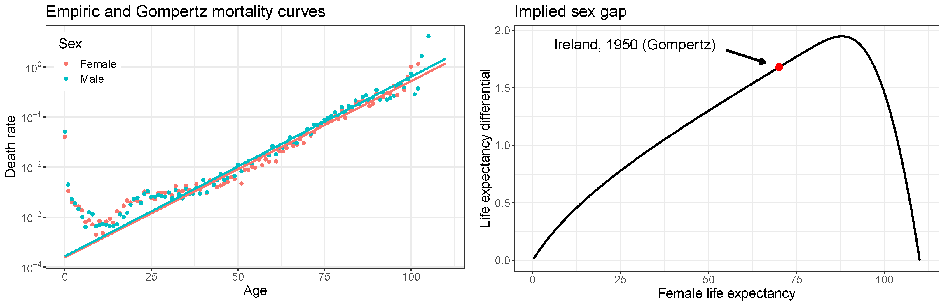
4. The Dynamic Gompertz Model

Parametric models can be used for mortality projections by letting calendar year enter the model through its parameters. That is, for each calendar year the parameters of the model are estimated and then viewed as stochastic processes, forecasted by standard time series methods. By linking the stochastic processes driving the models of different populations, coherence and other dependency structures can be achieved, see e.g., [8,9,13]. In this section, we analyze a particularly simple, coherent mortality model of this type. The model is too simple to be of practical use, but it is useful as an illustration of the sex gap trajectories implied by coherence.

4.1. The Model

The Gompertz mortality law prescribes that mortality increases exponentially,
μ ( x ) = e α + β x , 0 x ω .
This mortality profile is a remarkably good fit to adult mortality from age 20, say, onwards. For younger ages, and in fact also for very old ages, the profile is not appropriate. A simple two-sex model for adult mortality can be constructed by fitting a Gompertz law to period, sex-specific mortality data resulting in estimated coefficients ( α t , g , β t , g ) for g { f , m } and t ranging over the years in the estimation window.
If the parameters are modeled as random walks with the same drift for both sexes, the median forecast for population g becomes
μ ¯ g ( x , T + h ) = exp α T , g + β T , g x + h ( ξ α + ξ β x ) ,
where T denotes the projection jump-off year, h N 0 is the forecasting horizon, and  ξ α and ξ β are the (shared) drift terms of the α - and β -processes, respectively. By design, the forecasts in (21) are (strongly) coherent since the mortality sex ratios do not depend on h,
μ ¯ m ( x , T + h ) μ ¯ f ( x , T + h ) = exp ( α T , m α T , f ) + ( β T , m β T , f ) x = c ( x ) .
More complicated time-series models could also be used, but the current structure suffices for our purposes. Note that although h is assumed non-negative, we can evaluate (21) for all values of h. Specifically, we can think of a forecast as the right tail of an implied surface obtained by letting h range over all integers, negative and positive.

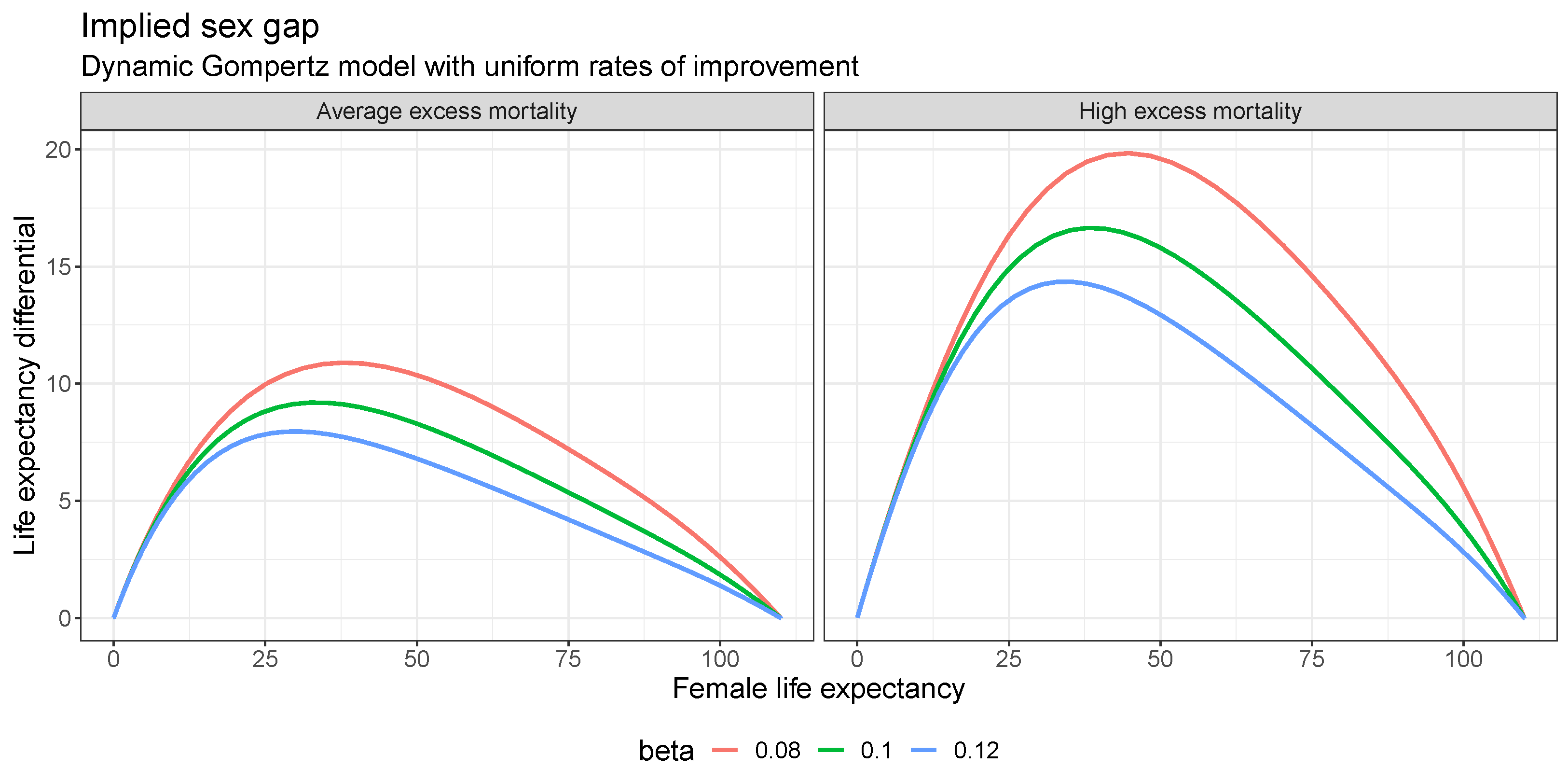
4.2. Sex Gap Unimodality under Uniform Rates of Improvement

Assuming uniform rates of improvement, the continuous-time analog of the dynamic Gompertz model is given by
μ ( x , t ) = e α + β x ρ t , 0 x ω ,
with level parameter α , slope parameter β > 0 , and rate of improvement ρ > 0 . As in Section 3.3, let μ f ( x , t ) = μ ( x , t ) and μ m ( x , t ) = μ ( x , t ) c ( x ) , where c ( x ) = exp ( Δ α + Δ β x ) , with  Δ β > β , such that μ m is also of form (23) with positive slope. Thus, mortality for both sexes follow a Gompertz mortality schedule with, in general, differing levels and slopes.
The cumulative death rate is
I ( x , t ) = 0 x μ ( u , t ) d u = e α ρ t ( e β x 1 ) / β ,
while its inverse for fixed time t is I 1 ( x , t ) = log ( 1 + x β / ( e α ρ t ) ) / β , whereby
μ ( I 1 ( x , t ) , t ) = e α ρ t + β x .
It follows that
x log μ m ( I m 1 ( x , t ) , t ) μ f ( I f 1 ( x , t ) , t ) = e α ρ t Δ β + β ( 1 e Δ α ) e α ρ t + β x e α + Δ α ρ t + ( β + Δ β ) x .
In practice, we typically find excess male mortality relative to female mortality with Δ α > 0 and Δ β < 0 , that is, the level is higher for males than for females, but the curve is less steep. In this situation, the right-hand side of (26) is negative, since the numerator is negative while the denominator is positive. It then follows from Theorem 1 that the sex gap is strictly unimodal.
We note that Theorem 1 only provides sufficient conditions for unimodality. For instance, having c ( x ) < 1 at high ages does not imply that unimodality of the gap will not occur. In fact, using empiric estimates we typically have this situation, but still the sex gap is unimodal.

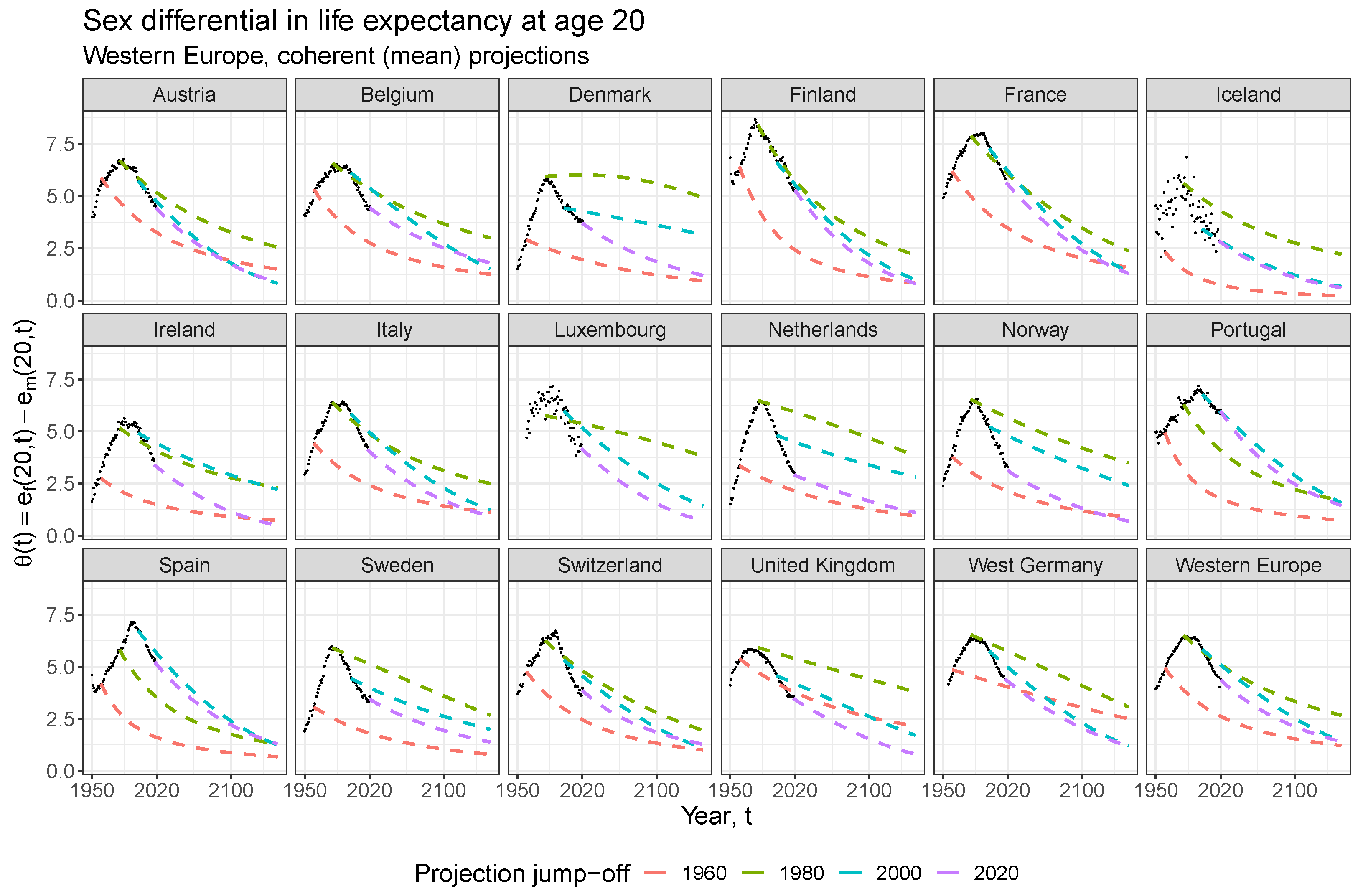
4.3. Sex Gap Trajectories

We define the sex gap trajectory as the pairs of female life expectancy and sex gap that can occur together on a given two-sex mortality surface,
T = { ( e f ( 0 , t ) , θ ( t ) ) : t R } ,
where as usual θ ( t ) = e f ( 0 , t ) e m ( 0 , t ) denotes the life expectancy differential (sex gap). In the continuous-time version of the dynamic Gompertz model, we have
μ f ( x , t ) = e α ρ t e β x , μ m ( x , t ) = e α ρ t e β x e Δ α + Δ β x .
Since ρ > 0 , we see that as t goes from minus infinity to plus infinity the common factor, exp ( α ρ t ) , takes all values in ( 0 , ) , regardless of the value of α and ρ . It follows that for the dynamic Gompertz model the sex gap trajectory is a function of the female slope parameter and excess mortality only, i.e.,  T = T ( β , Δ α , Δ β ) .
Based on mortality data from Western Europe 1950–2020, estimates of β are in a narrow range around 0.10 , while excess mortality shows greater variability from country to country and over time. Figure 4 shows two sets of trajectories for typical values of β ; the left plot corresponds to the average male excess mortality profile in the data, and the right plot corresponds to very high male excess mortality, as seen in, e.g., Finland.
We notice that although the size of the sex gap is different in the two plots, the overall shape of the trajectory is almost the same in all cases. In particular, we notice that the sex gap peaks when female life expectancy is in the range 30 to 50 years. This means that if a dynamic Gompertz model is fitted to data and forecasts are produced from a jump-off year where female life expectancy is larger than 50 years then the model will forecast a closing sex gap; at least if the slope parameters are relatively constant (i.e., if  ξ β 0 ).
Note that the speed with which the sex gap trajectory is traversed in the forecast depends on how fast female life expectancy evolves. We only know that as female life expectancy increases beyond 50 years, the sex gap closes. Since female life expectancy will not increase linearly, the shape of the sex gap in the forecast will typically not resemble the shape of the sex gap trajectories in Figure 4.
That the coherent, dynamic Gompertz model typically produces narrowing sex gaps also for age-dependent rates of improvement, is illustrated in Figure 5. The forecasts are produced by (21) for dynamic Gompertz models fitted to different countries in different periods. The Gompertz models are calibrated using data in the age range { 20 , , 100 } to avoid the poor fit at younger ages to influence parameter estimates; for the same reason we look at the life expectancy differential at age 20, instead of at birth. Parameters of the Gompertz models are estimated by maximum likelihood assuming independent, Poisson-distributed death counts, D ( x , t ) | E ( x , t ) Pois ( E ( x , t ) exp ( α t + β t x ) ) . The model’s parameters are calibrated to the latest 30 years of data available before projection jump-off. If data do not exist for all 30 years, only available data are used. We estimate and project the models for all countries in Western Europe and for periods with jump-off in 1960, 1980, 2000, and 2020, respectively.
As seen, almost all forecasts in Figure 5 produce narrowing gaps. In some periods the forecasts provide a good description of the future, e.g., the recent forecasts for Finland, France, Portugal and Spain, but in most cases the forecasted sex gap does not provide a sensible continuation of the historic trend. The problem is, that the behavior of data leading up to the jump-off year matters very little; it is the assumed coherence in the forecasts that produces the (implied) unimodal sex gap trajectory and it is the fact that female life expectancy is larger than 50 years at all jump-offs that places us on the declining part of that trajectory.
We note in closing, that the dynamic Gompertz model does not always forecast closing sex gaps. Periods with little or no mortality improvements for males (Denmark, 1980), or male mortality being very close to female mortality can lead to an increasing sex gap at jump-off. In the latter case, the peak of the implied sex gap trajectory can occur at a much higher age than indicated in Figure 4, cf. Box 2 “The outlier Ireland” for an example of this rarely happening situation.

5. The Forecast of Closing Sex Gaps by Coherent Mortality Models

In the previous section we demonstrated that the dynamic Gompertz model typically forecasts closing sex gaps, both under uniform rates of improvement, as predicted by Theorem 1, but also under age-dependent rates of improvement. In this section, we show that more “realistic”, coherent mortality models behave qualitatively similar to the dynamic Gompertz model. On this basis, we conclude that closing sex gaps is indeed a general feature of coherent models. The analysis is in two parts. First, we relax the parametric structure of the Gompertz curve but keep the uniform rate of improvement. Second, we show closing sex gaps for coherent, semi-parametric models with age-dependent rates of improvement.

5.1. Location of the Sex Gap Zenith under Uniform Rates of Improvement

Based on the dynamic Gompertz model, we concluded in Section 4.3 that for Western European data the implied sex gap peaks at an earlier age than the observed female life expectancy, leading to closing sex gap forecasts. One might object to this analysis that the Gompertz model allows for only a very limited set of mortality profiles, and that the conclusion implicitly rests on this fact. Below, we extend the analysis to general, smooth mortality profiles, retaining the assumption of uniform rates of improvement.
Consider a (strongly) coherent mortality surface with female and male mortality of the form μ f ( x , t ) = μ f ( x , T ) exp ( ρ ( t T ) ) and μ m ( x , t ) = μ f ( x , t ) c ( x ) , respectively, where T is a fixed year, μ f ( x , T ) is the female mortality at age x in year T, c ( x ) is the male excess mortality at age x, and  ρ > 0 is the (uniform) rate of improvement.
Recall from Equation (27) that the sex gap trajectory is defined as the set of female life expectancies and sex gaps that can occur together when t varies. By the same argument as in Section 4.3, this set does not depend on the rate of improvement. In other words, assuming a uniform rate of improvement, the sex gap trajectory depends only on the female mortality profile in any given year and the excess mortality profile. In particular, for any female mortality profile, μ f ( · , T ) , and any c-profile, we can define the (implied) sex gap zenith,
( a max , θ max ) = ( e f ( 0 , t max ) , θ ( t max ) ) , w h e r e   t max = arg max θ ( t ) ,
as the female life expectancy when the sex gap is at its maximum and the corresponding (maximal) value of the sex gap. The notation ( a max , θ max ) is chosen to reflect the abscissa and ordinate at the maximum point, cf. Figure 4.
We compute and compare ( a max , θ max ) for (i) a Gompertz model and (ii) a graduated mortality curve, where the mortality curves obtained by graduation closely represent the true underlying death rates. In short, the graduation procedure smooths the empirical death rates by a cubic smoothing spline, while the Kannisto model of old-age mortality is used at ages 80 and above. Further details are provided Appendix B.
The sex gap zenith is presented in Table 1 for the two models for the countries in Western Europe. For given year, mortality data for that year only is used to estimate female and male mortality profiles from which the c-profile is derived. Next, assuming a uniform rate of improvement, the implied sex gap trajectory (27) can be computed. Finally, the female life expectancy and the size of the sex gap at the zenith (29) of the trajectory are found. The computation is performed on data from three calendar years that captures the different epochs of the period. In the first year, 1950, all countries are on the widening part of the observed θ -curve. The second year, 1985, is the middle of the period where the observed θ -curve peaks, while the third year, 2020, is on the narrowing part of the curve, cf. Figure 1. If a country does not have data at one or both of the endpoints, the nearest data point is used instead.
BOX 2. THE OUTLIER IRELAND
The only outlier in Table 1 is Ireland, 1950. In this year, the observed life expectancy for females is 66.7 years, but according to Table 1, this is well below a max . Ireland is rather unique in a demographic context. Men outlived women at the beginning of the 20th century, and by the 1930s, Ireland was the only country in the West with higher survival rates for men than for women at any age [35]. This pattern has taken a while to reverse, and even though female mortality is lower than male mortality in 1950 (at most ages), the curves lie almost directly on top of each other as seen in Figure 6. Interestingly, this fact makes the sex gap widen for a prolonged period, that is, the slope of θ is rather moderate before reaching the turning point. Once the turning is passed, however, the gap will close quite rapidly; the slope on the narrowing part is much steeper compared to the slope on the widening part of the curve as seen in Figure 6. This feature needs to be understood in the context of life span disparity, e , and the maximum attainable age, ω . Because the mortality profiles are similar not only in slope but also in level, e f stays higher than e m for longer. Female life expectancy at the turning point, a max , is, therefore, closer to ω than had the mortality levels been further apart, causing the subsequent “catch-up” to happen much faster.
The Gompertz model predicts a female life expectancy of around 30–40 years when the sex gap is at its zenith, varying slightly from country to country and period to period. For comparison, observed female life expectancy in 1950 is between 61.0 (Portugal) and 73.6 (Iceland) and increasing over the period. Thus, all countries are on the declining part of the implied θ -curve, and continued improvements in mortality will further narrow the gap. The only exception is Ireland, see Box 2.
Because the Gompertz curve constitutes a highly stylized mortality profile, the life expectancy predictions from this model are fairly consistent across the different countries and periods. The graduated mortality curve is more flexible, resulting in more diverse predictions, in particular, regarding the female life expectancy at the sex gap zenith. The overall result is, however, qualitatively the same; with the exception of Ireland, the implied sex gap peaks when female life expectancy is below that observed at the estimation year (not shown). The takeaway message is that for essentially all countries and jump-off years, both models project narrowing sex gaps.
Figure 6. Mortality and implied sex gap for Ireland, 1950. In the left panel, the Gompertz fit is superimposed as solid lines.
Forecasting 04 00045 g006

5.2. Coherence Implies Closing Sex Gaps

Until now we have demonstrated sex gap unimodality and closing sex gap forecasts under conditions imposed for mathematical tractability. In particular, strong coherence and uniform rates of improvement. Of course, coherent mortality models used in practice are neither strongly coherent, nor do they have uniform rates of improvement. Nevertheless, the conclusion extends to “realistic”, coherent models also, and for the same reason. Calibrated to Western European mortality data, the sex gap implied by the models peaks when female life expectancy is (much) lower than levels observed after the Second World War.
Table 2 presents the slope of the sex gap following projection jump-off based on the dynamic Gompertz model (21), the Li-Lee model (11), and the product ratio model of Hyndman et al. [3] for different jump-off years. For the Li-Lee model (11), we use AR(1)-processes to describe the sex-specific time-varying indices. The product ratio model is fitted and forecasted using the Demography package (available on CRAN) in R.
Except for the United Kingdom, the actual sex gap was widening at all jump-off years, cf. Figure 1. Nevertheless, essentially all forecasts predict a narrowing sex gap. Further, for those (few) forecasts where the gap is projected to widen, the historical trend is not reproduced. Rather, the apex of θ is predicted to be in the near future with a gap that remains approximately constant on a short horizon (not shown); the forecast trajectories resemble that of Denmark, 1980 seen in Figure 5 (green, dashed line).
In semi-parametric mortality models, e.g., the Lee–Carter model [2] or the Li-Lee model [1], the fit to data is typically good due to a large number of parameters. Even parsimonious model structures such as the dynamic Gompertz model can capture many observed mortality patterns when parameters are allowed to vary freely. Consequently, in the estimation window, most mortality models allow flexible, if not freely varying, rates of improvement, ρ ( x , t ) . In the forecasting region, however, the improvement rates are often, directly or indirectly, constrained by (i) assuming temporal constancy, e.g., in models of the Lee–Carter type, and (ii) by imposing coherence:
ρ ( x , t ) Time invariance ρ ( x ) Coherence ρ f ( x ) ρ m ( x ) .
Both assumptions might be at odds with (recent) trends in data, resulting in death rate (median) trajectories that may not conform with those observed in the past. Relaxing the assumption of time-invariant improvement rates can be achieved by various techniques, for example, by imposing convergence to a long-term target [36], or applying frailty theory [37]. This, however, is not the focus of the present paper.
Although, formally only a condition in the limit, the coherence assumption built into many multi-population mortality models all but eliminates the ratio effect, identified by Glei and Horiuchi [15] and Cui et al. [25] as the main driver of the widening sex gap in Western Europe until the 1980s, cf. Section 2.2. In periods where the sex gap is narrowing, the ratio effect is less important and the coherence assumption agrees more with observed data. Narrowing sex gap projections are produced as intended but are not guaranteed to replicate the latest trends, cf. Figure 5. In summary, the implied sex gap trajectory of coherent models, being driven mainly by the level effect, is too inflexible to adequately describe and forecast the sex gap evolution since 1950.

5.3. Does Coherence Deserve Its Special Status?

The fact that the sex gap narrows in coherent projections at essentially all levels of mortality observed in the West over the last 70 years challenges the desirability of coherence as a modeling goal and adds to the recent criticism of coherence raised by Hunt and Blake [12] and Jarner and Jallbjørn [13]. At the time of its development, coherence coincidentally appeared as a desirable property that (to some extent) continued the narrowing of the sex gap that had been observed for some time, unlike most independent methods that projected widening or diverging gaps, see for example Figure 5 in Hyndman et al. [3]. One can understand that Hyndman et al. [3] and others concluded that coherent forecasts were an improvement over independent forecasts, but this verdict seems somewhat anchored in the sex gap decline of the time. Imagine standing in a year between 1950–1980, observing sharp transitions from widening to narrowing gaps such as those in Figure 5. It then seems far less obvious that coherence is a property one should impose on a model and certainly questions whether coherence deserves the special status it has been given.
From the adversarial perspective, it is—at least in theory—possible for coherent models to accommodate temporary ratio effects of varying (but bounded) size and thereby produce trends in the sex gap that are in keeping with those recently observed. In most applications, however, the ratio effect diminishes quickly, leading to a misalignment between historic and projected trends as demonstrated in Table 2. Arguably, a diminishing ratio effect is intentional, because otherwise, the rationale for imposing coherence would be undermined. Even though coherence may be a sensible restriction to impose when extrapolating the present mortality regime (for some populations), it does not seem to be so historically and may not be so in the future either. In our view, this suggests a revision of coherence as the guiding principle for multi-population mortality modeling.
Moreover, as is also pointed out by Jarner and Jallbjørn [13], coherence seems too tailored to the log-linear common factor models for which the property was introduced. Even though single population models can be coupled via cointegration techniques to achieve coherence, the choice of scale, i.e., ratios of mortality rates, remains somewhat arbitrary and effectively restricts the coherence label to models of the Lee–Carter type. Therefore, we see a need for a broader definition that covers a larger class of models and permits less restrictive dependency structures.
As a minimum, the coherence requirement should be relaxed to allow for observed patterns of covariation to continue in forecasts. A possible approach to tackle this issue could be to redefine coherence into a property that concerns modeling on the parameter scale rather than modeling on the (log) data scale. In particular, it seems more natural to identify cointegrating relations between (time-varying) parameters, i.e., identifying linear combinations of the parameters that are stationary, rather than requiring mean-reversion of mortality log differences. For further discussion on this point, see Jarner and Jallbjørn [13].

6. Conclusions

The notion of coherence has been one of the most influential ideas in multi-population mortality modeling. When projecting groups of related populations, e.g., males and females, or countries of similar affluence, which have evolved in parallel in the past, it is natural to expect these populations to “stay together” in the future also. Coherence solves the problem of diverging, or crossing, forecasts that can arise when projecting, even very similar, populations separately. It does so by requiring converging mortality ratios, or, equivalently, asymptotically equal rates of improvement at each age. At first sight, this seems an innocent and reasonable requirement, but in practice coherent models enforce a rigid structure on the forecasts that can be at odds with trends in data.
In this paper we discussed the implications of coherence in two-sex mortality models with focus on the dynamics of the sex differential in life expectancy (sex gap). We provided both theoretical and empirical evidence to support the conclusion that coherent models forecast closing sex gaps for Western European countries for almost all jump-off years since 1950. Despite the fact that the actual sex gap was widening until the 1980s. Coincidentally, coherence was introduced after almost 20 years of narrowing sex gaps, and a continued sex gap closing was seen as a desirable feature of coherent models. However, the inadequacy of coherent models in the first half of the period from 1950 till today, lead us to question coherence as a general modeling principle.
Technically, we prove in the paper that strongly coherent models with a uniform rate of improvement produce a unimodal sex gap trajectory. Further, we demonstrate that for Western European levels of male excess mortality (relative to female mortality) the implied sex gap trajectory typically peaks when female life expectancy is in the range 30 to 50 years. Although formally proven only for a specific subclass of coherent models, this insight applies in much greater generality and it explains why forecasts from coherent two-sex models are almost always on the declining part of the trajectory.
We also discussed the effects responsible for the observed widening and narrowing sex gap in Western Europe from 1950 till today. In particular, with appeal to Glei and Horiuchi [15] we identified changing sex ratios (the ratio effect) as the main driver of the widening sex gap, and differential dispersion combined with general improvements (the level effect) as the main driver of the subsequent narrowing of the sex gap. In light of the similarity between the observed and implied sex gap trajectories in Figure 1 and Figure 4, respectively, it is a priori surprising that coherent models cannot be used to describe the observed sex gap dynamics over the entire period. However, the implied sex gap trajectory peaks too early, in terms of female life expectancy, and therefore cannot be aligned with the widening part of the observed sex gap trajectory. Moreover, even on the narrowing part of the observed sex gap trajectory, coherent forecasts often have a kink at jump-off, see Figure 5. In conclusion, the implied sex gap trajectory of coherent models being driven purely, or mainly, by the level effect is not sufficiently flexible to describe the observed sex gap dynamics.
To prove unimodality of the sex gap, we relied on the assumption that life expectancies are bounded from above, implying that we eventually approach a life expectancy plateau and that the sex gap therefore vanishes in the limit. Even though life expectancy does not appear to be approaching a maximum at present [38] and even though women have been shown to “always” live longer than men [33,34], it does seem reasonable that a biological or genetic barrier to an infinite lifespan exists; however, if an upper limit does not exist a vanishing sex gap is not guaranteed. It is also conceivable that the present level of old-age mortality acts similar to a de facto barrier, but that continued improvements can “break through” the barrier and move it to even higher ages.
Although we have presented the results and the analysis as pertaining to coherent models and their properties, the unimodality result can also be given a real-world interpretation. In Western Europe, males have historically had lower rates of improvement than females, but currently the two sexes enjoy similar rates of improvement. Combined with the unimodality result, this indicates that the observed sex gap will continue to close in the future but it also points to factors that need to change for the gap to start widening again. That is, (i) if mortality undergoes a (perhaps temporary) regime change in which female rates of improvement substantially outweigh male improvements, for instance, if certain diseases that primarily target females are reduced or eradicated, or if sex-specific risk behavior changes in favor of women; (ii) if the current lifetime barrier is broken through, the sex gap dynamics could “start over” and result in a multimodal curve similar to that exemplified in Figure 3. It is also conceivable that a widening gap in favor of men could be brought about. This can happen, e.g., if the sex-specific mortality curves continue to steepen in such a way that high-age male mortality falls below high-age female mortality.
The paper focused on coherence in two-sex models. However, our main result applies also to other coherent, multi-population models whenever an ordering of the population-specific mortality rates exists. A noteworthy instance is mortality rates between different socio-economic groups, a case that has attracted much recent attention, see e.g., Bennett et al. [39], Cairns et al. [40]. Historically, the life expectancy gap between the most and least affluent has widened for some time, and the trend is expected to continue over the coming years by domain experts. However, under the assumption of coherence, the gap may inadvertently be projected to close right after projection jump-off. Other applications with mortality orderings expected to persist over time include modeling of rich countries relative to poor countries, insured lives relative to non-insured lives, and smokers relative to non-smokers. In all these cases, coherent models are likely to produce immediately narrowing gaps irrespective of the historic development leading up to jump-off.
Finally, since the main result hinges on excess mortality of one population relative to another, it cannot be applied to situations where such an ordering does not exist. For example, when modeling a group of neighboring countries of similar affluence, we cannot conclude that this will generally lead to closing gaps for all pairs of countries. Arguably, even if we could, narrowing gaps would perhaps be less of a worry in this context, at least in the long run.

Author Contributions

Conceptualization, S.J. and S.F.J.; Methodology, S.J. and S.F.J.; Validation, S.J. and S.F.J.; Writing—original draft preparation, S.J.; Writing—review and editing, S.F.J.; Visualization, S.J. All authors have read and agreed to the published version of the manuscript.

Funding

This research was funded by Innovation Fund Denmark (IFD) grant number 9065-00135B.

Institutional Review Board Statement

Not applicable.

Informed Consent Statement

Not applicable.

Data Availability Statement

The data used in this paper are available at https://www.mortality.org (accessed on 4 January 2022).

Acknowledgments

The authors wish to thank three anonymous referees for helpful comments that improved the manuscript.

Conflicts of Interest

The authors declare no conflict of interest.

Appendix A. Proofs and Lemmas

Appendix A.1. Stochastic Dominance

The following lemma gives a general result that is used to assess the sign of the second derivative of the sex gap at a stationary point. The lemma has ties to the concept of stochastic dominance, see e.g., Lindvall [41]. We say that a real-valued random variable Y stochastically dominates another real-valued random variable X if P ( Y z ) P ( X z ) for all z. Informally, this means that the distribution of X is to the left of the distribution of Y. Various inequalities based on this partial ordering can be derived. The result we need is stated below.
Lemma A1.
Let f 1 and f 2 be strictly positive functions with compact support [ 0 , K 1 ] and [ 0 , K 2 ] , respectively, with 0 < K 1 < K 2 < , satisfying
0 K 1 f 1 ( x ) d x = 0 K 2 f 2 ( x ) d x .
Assuming that f 1 and f 2 have continuous first derivatives such that
x log f 1 ( x ) x log f 2 ( x ) f o r   0 < x < K 1 ,
then for any strictly increasing, differentiable function h : [ 0 , K 2 ] R ,
0 K 1 h ( x ) f 1 ( x ) d x < 0 K 2 h ( x ) f 2 ( x ) d x .
Proof. 
Let m denote the common value in (A1), and let ν 1 and ν 2 denote measures concentrated on [ 0 , K 1 ] and [ 0 , K 2 ] , respectively, so that g 1 ( x ) = f 1 ( x ) / m and g 2 ( x ) = f 2 ( x ) / m are the Radon–Nikodym derivatives of ν 1 and ν 2 with respect to Lebesgue measure. Further, let G 1 ( x ) = 0 x g 1 ( u ) d u and G 2 ( x ) = 0 x g 2 ( u ) d u be the corresponding cdf’s.
It suffices to show that G 2 ( x ) G 1 ( x ) , x [ 0 , K 2 ] , with strict inequality at some x, because then
0 K 1 h d ν 1 0 K 2 h d ν 2 = 0 K 1 0 x h ( u ) d u d G 1 ( x ) 0 K 2 0 x h ( u ) d u d G 2 ( x ) = 0 K 1 h ( x ) 1 G 1 ( x ) d x 0 K 2 h ( x ) 1 G 2 ( x ) d x = 0 K 2 h ( x ) G 2 ( x ) G 1 ( x ) d x < 0 ,
and (A3) follows immediately. In the above, the first equality follows by writing
h ( x ) = h ( 0 ) + 0 x h ( u ) d u ,
and the second by reversing the order of integration. The latter computation is valid by Tonelli’s theorem since h is non-negative.
We know that G 1 ( 0 ) = G 2 ( 0 ) = 0 and G 2 ( x ) G 1 ( x ) = 1 for x [ K 1 , K 2 ] . For 0 < z < w < K 1 we have from (A2) that
log g 1 ( w ) g 1 ( z ) = z w x log f 1 ( x ) d x z w x log f 2 ( x ) d x = log g 2 ( w ) g 2 ( z ) ,
and thereby g 1 ( w ) / g 1 ( z ) g 2 ( w ) / g 2 ( z ) , or, equivalently, g 2 ( z ) / g 1 ( z ) g 2 ( w ) / g 1 ( w ) . Hence, r ( x ) = g 2 ( x ) / g 1 ( x ) is monotonically increasing on ( 0 , K 1 ) . Define the sets
A = { x x ( 0 , K 1 ) , r ( x ) < 1 } ,
B = { x x ( 0 , K 1 ) , r ( x ) = 1 } ,
C = { x x ( 0 , K 1 ) , r ( x ) > 1 } ,
that collectively cover ( 0 , K 1 ) . Since
0 K 1 g 1 ( x ) d x = 0 K 2 g 2 ( x ) d x > 0 K 1 g 2 ( x ) d x = 0 K 1 r ( x ) g 1 ( x ) d x ,
A cannot be empty. Due to the monotonicity of r, C cannot be empty without B being empty. If both B and C are empty or if only C is empty, we have that
G 2 ( x ) = 0 x r ( u ) g 1 ( u ) d u < 0 x g 1 ( u ) d u = G 1 ( x ) ,
for all x ( 0 , K 1 ) . If C is non-empty, suppose for contradiction that there exists an x C for which G 2 ( x ) G 1 ( x ) . Then, due to the monotonicity of r, we would have G 2 ( K 1 ) G 1 ( K 1 ) , but this contradicts (A10). Thus, we conclude that G 2 ( x ) < G 1 ( x ) for all x ( 0 , K 1 ) . □

Appendix A.2. Proof of Theorem 1

For ease of reference, we recall the central definitions and assumptions used in Theorem 1. Let μ : [ 0 , ω ] × R ( 0 , ) be a twice continuously differentiable function satisfying
lim t μ ( x , t ) = , and lim t μ ( x , t ) = 0 .
Let μ f ( x , t ) = μ ( x , t ) and μ m ( x , t ) = μ ( x , t ) c ( x ) denote female and male mortality, respectively. Let θ ( t ) = e f ( 0 , t ) e m ( 0 , t ) denote the sex gap. Note that θ is twice continuously differentiable. The proof of Theorem 1 relies on Lemma A1 and the following two lemmas.
Lemma A2.
Assume c ( x ) > 1 for all x. The sex gap, θ, attains its global maximum on R . In particular, θ has at least one stationary point.
Proof. 
We first note that θ ( t ) > 0 for all t R with limits
lim t θ ( t ) = lim t θ ( t ) = 0
This follows from (A12) and the assumption μ f ( x , t ) < μ m ( x , t ) for all x and t. Choose an arbitrary real number t 0 R . Because the limit of θ in either end of the real line is zero, there exist numbers < t l < t 0 < t u < such that θ ( t ) θ ( t 0 ) for t t l , and θ ( t ) θ ( t 0 ) for t t u . Since θ is continuous it attains a maximal value at, say, t m on the compact interval [ t l , t u ] , cf. Rudin [42] Theorem 4.16. This is also the global maximum by construction since t 0 [ t l , t u ] . Hence, since θ is continuously differentiable, it follows that θ ˙ ( t m ) = 0 . □
Lemma A3.
Assume c ( x ) > 1 for all x. If stationary points of θ are local maxima, that is, if
t R : θ ˙ ( t ) = 0 θ ¨ ( t ) < 0 ,
then θ is strongly unimodal on R .
Proof. 
Assume (A14) holds. We start by showing that θ can have at most one stationary point, or equivalently, that θ ˙ can have at most one root. Assume for contradiction that θ ˙ has at least two roots a , b R with a < b . By (A14), θ ¨ ( a ) < 0 and therefore there exists ε > 0 such that θ ˙ is strictly negative on ( a , a + ε ] . Let c = inf { t > a : θ ˙ ( t ) 0 } be the first time θ ˙ passes zero after a. The set defining c is disjoint with ( a , a + ε ] and it is non-empty because it contains b, by assumption. In particular, c a . By continuity, θ ˙ ( c ) = 0 , because if θ ˙ ( c ) > 0 there would exist a + ε < t < c with θ ˙ ( t ) = 0 contradicting the definition of c, see e.g., Rudin [42] Theorem 5.12. For the same reason, θ ˙ ( t ) < 0 for all t ( a , c ) . Now, since θ is twice differentiable at c, the limit
lim t c θ ˙ ( t ) θ ˙ ( c ) t c = lim t c θ ˙ ( t ) t c
exists and equals θ ¨ ( c ) ; however, since θ ˙ ( t ) < 0 in an interval to the left of c, we find θ ¨ ( c ) 0 contradicting (A14). We conclude that θ can have at most one stationary point.
By Lemma A2 we know that θ attains its unique maximum at some t m R , and as just shown this is the only stationary point. Consequently, θ ˙ ( t ) > 0 for all t < t m , and θ ˙ ( t ) < 0 for all t > t m , and we conclude the θ is strongly unimodal. □
Theorem 1.
Assume t log μ ( x , t ) = ρ ( t ) > 0 for all x, i.e., the rates of improvement is the same for all ages and strictly positive at all times. If c ( x ) > 1 for all x, and
x log μ m ( I m 1 ( x , t ) , t ) μ f ( I f 1 ( x , t ) , t ) 0 ,
for all t R , and all x where the argument is defined, then θ is strictly unimodal on R .
Proof. 
By Lemma A3 it suffices to prove condition (A14). The first and second derivatives of θ are given by
θ ˙ ( t ) = ρ ( t ) 0 ω I f ( x , t ) e I f ( x , t ) I m ( x , t ) e I m ( x , t ) d x ,
θ ¨ ( t ) = ρ ˙ ( t ) 0 ω I f ( x , t ) e I f ( x , t ) I m ( x , t ) e I m ( x , t ) d x + ρ 2 ( t ) 0 ω ( I f 2 ( x , t ) I f ( x , t ) ) e I f ( x , t ) ( I m 2 ( x , t ) I m ( x , t ) ) e I m ( x , t ) d x .
Fix a t R for which θ ˙ ( t ) = 0 . We then obtain from (A17) that θ ¨ ( t ) reduces to
θ ¨ ( t ) = ρ 2 ( t ) 0 ω I f 2 ( x , t ) e I f ( x , t ) I m 2 ( x , t ) e I m ( x , t ) d x .
Thus, to establish (A14) it suffices to establish that the integral in (A19) is negative.
The proof relies on an invocation of Lemma A1. To bring θ ˙ ( t ) and θ ¨ ( t ) on a form more suitable for this purpose, we introduce, with slight abuse of notation, the variable transform z = I ( x , t ) and write
θ ˙ ( t ) = ρ ( t ) 0 I f ( ω , t ) f f ( z , t ) d z 0 I m ( ω , t ) f m ( z , t ) d z ,
θ ¨ ( t ) = ρ 2 ( t ) 0 I f ( ω , t ) z f f ( z , t ) d z 0 I m ( ω , t ) z f m ( z , t ) d z ,
where f g ( z , t ) = z e z / μ g ( I g 1 ( z , t ) , t ) , for g { f , m } , is the (transformed) integrand of the integrals in (A17). We note that I is invertible by the inverse function theorem, see e.g., Rudin [42] Theorem 9.24.
Now, since assumption (A2) of Lemma A1 is equivalent to assumption (18) of Theorem 1, that is,
z log f f ( z , t ) f m ( z , t ) = z log μ m ( I m 1 ( z , t ) , t ) μ f ( I f 1 ( z , t ) , t ) 0 ,
and since μ m ( x , t ) > μ f ( x , t ) for all x implies that I m ( ω , t ) > I f ( ω , t ) , we can invoke Lemma A1 to obtain that
0 I f ( ω , t ) z f f ( z , t ) d z < 0 I m ( ω , t ) z f m ( z , t ) d z .
It immediately follows that the integral in (A21), and thereby the integral in (A19), is negative, and we are done. □

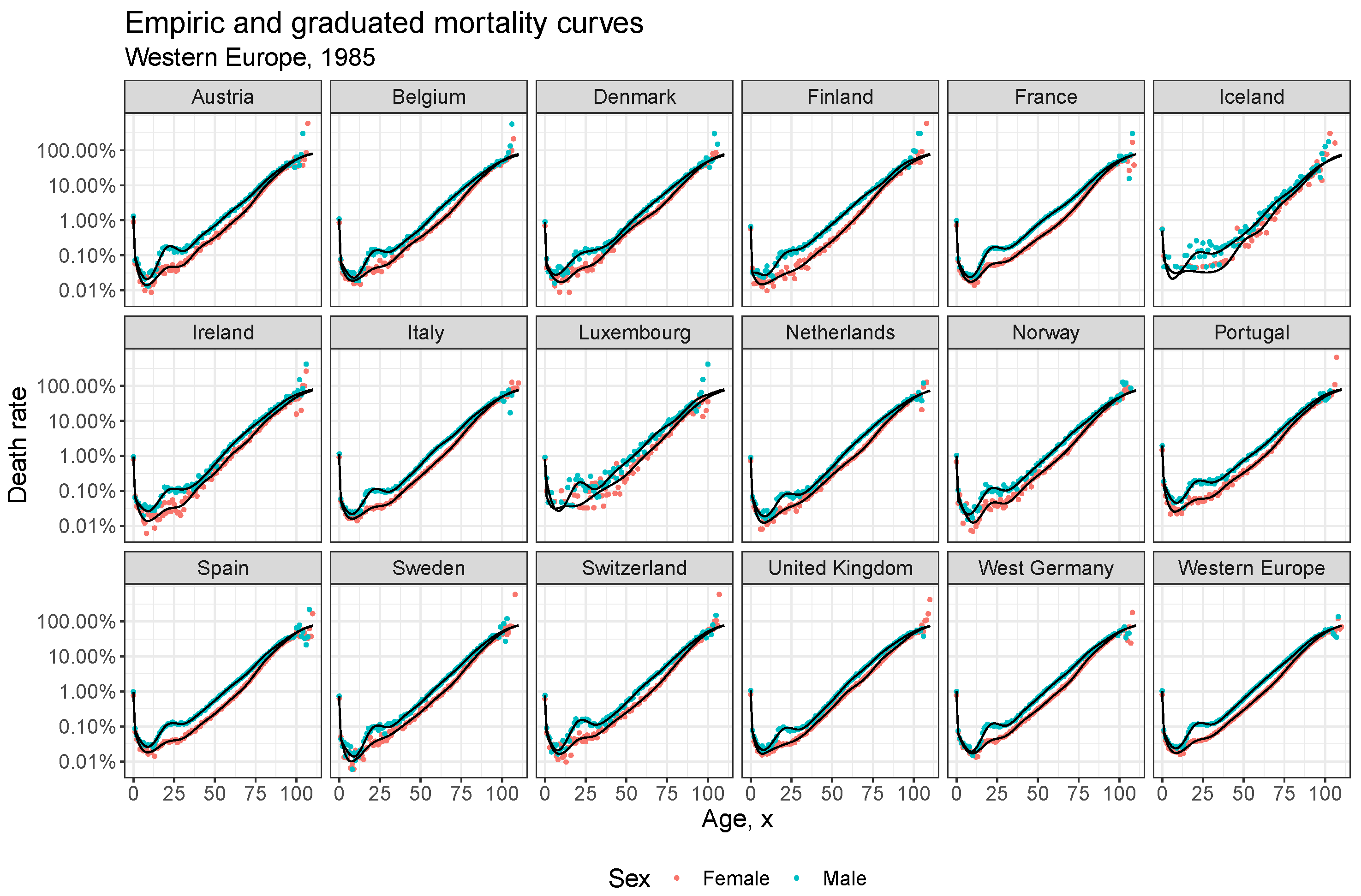
Appendix B. Graduation of μ(x)

Suppose we have data on deaths, D ( x ) , and exposures, E ( x ) , for integer ages x { 0 , , 110 } . By smoothing the empirical death rates, m ( x ) = D ( x ) / E ( x ) , we wish to obtain an improved representation of the true underlying mortality curve, μ ( x ) . An example of the graduation procedure described below applied to data is shown in Figure A1.
Figure A1. Empiric (dots) and graduated (line) death rates. The graduated mortality curve is computed through (A27).
Forecasting 04 00045 g0a1

Appendix B.1. General Smoothing

Within the observed age range (0–110) we fit a cubic smoothing spline to the observed death rates, i.e., we model m by an additive noise model m ( x ) = f ( x ) + ε ( x ) where ε ( x ) is assumed iid with mean zero and the cubic smoothing spline estimate f ^ of f minimizes
x X m ( x ) f ^ ( x ) 2 + λ f ^ ( u ) 2 d u
where the smoothing parameter λ is fitted through cross-validation and
X = { 0 , 1 , 10 , 20 , 30 , 40 , 50 , 60 , 70 , 80 , 110 }
is the set of knots used. From f ^ , we can obtain smoothed estimates μ ^ spline ( x ) = f ^ ( x ) for general (non-integer) x.

Appendix B.2. Old-Age Smoothing

For the highest ages, we smooth the mortality curve by fitting a logistic function to the observed death rates for ages 80 and above. That is, we fit the Kannisto model
logit μ ( x ; a , b ) = a + b ( x 80 ) ,
with parameters a , b R , cf. Thatcher et al. [43]. The parameters are found by maximizing a Poisson log-likelihood
log L ( a , b ) = x = 80 99 D ( x ) log μ ( x ; a , b ) E ( x ) μ ( x ; a , b ) ,
for data in the age-range 80–99. Substituting the maximum likelihood estimates a ^ and b ^ into (A25) yields smoothed death rates μ ^ logit ( x ) = μ ( x ; a ^ , b ^ ) .

Appendix B.3. Mortality for the Combined Curve

We calculate smooth death rates for the entire age range by the weighted average
μ ^ ( x ) = μ ^ spline ( x ) ( 1 w ( x ) ) + μ ^ logit ( x ) w ( x ) ,
with weights w ( x ) = min ( 1 , max ( ( x 80 ) / 20 , 0 ) ) for x [ 0 , 110 ] .

Appendix C. Life Expectancy under Piecewise Constancy

Suppose that mortality is piecewise constant over squares of the form [ x , x + 1 ) × [ t , t + 1 ) for integer ages x { 0 , , 110 } = X and calendar years t T , that is, suppose
μ ( x + Δ x , t + Δ t ) = μ ( x , t ) , Δ x , Δ t [ 0 , 1 ) ,
for all x X , t T . The assumption of piecewise constancy is convenient for many calculations of life table related quantities. In particular, for any integer age of truncation, ω { 0 , , 111 } , the (truncated) life expectancy can be evaluated analytically as:
e ( x , t ) = x ω e x y μ ( z , t ) d z d y = i = x ω 1 i i + 1 e x y μ ( z , t ) d z d y = i = x ω 1 i i + 1 e i y μ ( z , t ) d z d y e x i μ ( z , t ) d z = i = x ω 1 i i + 1 e μ ( i , t ) ( y i ) d y e j = x i 1 j j + 1 μ ( z , t ) d z = i = x ω 1 e μ ( i , t ) ( y i ) μ ( i , t ) i i + 1 e j = x i 1 μ ( j , t ) = i = x ω 1 1 e μ ( i , t ) μ ( i , t ) e j = x i 1 μ ( j , t ) .
We use ω = 110 throughout the paper.

References

  1. Li, N.; Lee, R. Coherent mortality forecasts for a group of populations: An extension of the Lee-Carter method. Demography 2005, 42, 575–594. [Google Scholar] [CrossRef] [PubMed]
  2. Lee, R.; Carter, L. Modeling and Forecasting U.S. Mortality. J. Am. Stat. Assoc. 1992, 87, 659–671. [Google Scholar] [CrossRef]
  3. Hyndman, R.J.; Booth, H.; Yasmeen, F. Coherent mortality forecasting: The product-ratio method with functional time series models. Demography 2013, 50, 261–283. [Google Scholar] [CrossRef]
  4. Li, J.S.H.; Hardy, M. Measuring Basis Risk in Longevity Hedges. N. Am. Actuar. J. 2011, 15, 177–200. [Google Scholar] [CrossRef]
  5. Li, J. A Poisson common factor model for projecting mortality and life expectancy jointly for females and males. Popul. Stud. 2013, 67, 111–126. [Google Scholar] [CrossRef] [PubMed]
  6. Zhou, R.; Wang, Y.; Kaufhold, K.; Li, J.S.H.; Tan, K.S. Modeling period effects in multi-population mortality models: Applications to Solvency II. N. Am. Actuar. J. 2014, 18, 150–167. [Google Scholar] [CrossRef]
  7. Kleinow, T. A common age effect model for the mortality of multiple populations. Insur. Math. Econ. 2015, 63, 147–152. [Google Scholar] [CrossRef]
  8. Jarner, S.F.; Kryger, E.M. Modelling adult mortality in small populations: The SAINT model. ASTIN Bull. J. IAA 2011, 41, 377–418. [Google Scholar] [CrossRef]
  9. Cairns, A.J.; Blake, D.; Dowd, K.; Coughlan, G.D.; Khalaf-Allah, M. Bayesian Stochastic Mortality Modelling for Two Populations. ASTIN Bull. 2011, 41, 29–59. [Google Scholar] [CrossRef]
  10. Börger, M.; Aleksic, M.C. Coherent projections of age, period, and cohort dependent mortality improvements. In Proceedings of the 30th International Congress of Actuaries, Washington, DC, USA, 26–30 March 2014. [Google Scholar]
  11. Shang, H.L.; Hyndman, R.J. Grouped functional time series forecasting: An application to age-specific mortality rates. J. Comput. Graph. Stat. 2017, 26, 330–343. [Google Scholar] [CrossRef] [Green Version]
  12. Hunt, A.; Blake, D. Identifiability, cointegration and the gravity model. Insur. Math. Econ. 2018, 78, 360–368. [Google Scholar] [CrossRef]
  13. Jarner, S.F.; Jallbjørn, S. Pitfalls and merits of cointegration-based mortality models. Insur. Math. Econ. 2020, 90, 80–93. [Google Scholar] [CrossRef]
  14. Trovato, F.; Lalu, N. Narrowing sex differentials in life expectancy in the industrialized world: Early 1970’s to early 1990’s. Soc. Biol. 1996, 43, 20–37. [Google Scholar] [CrossRef] [PubMed]
  15. Glei, D.A.; Horiuchi, S. The narrowing sex differential in life expectancy in high-income populations: Effects of differences in the age pattern of mortality. Popul. Stud. 2007, 61, 141–159. [Google Scholar] [CrossRef] [PubMed]
  16. Retherford, R.D. Tobacco smoking and the sex mortality differential. Demography 1972, 9, 203–215. [Google Scholar] [CrossRef]
  17. Mäkelä, P. Alcohol-related mortality by age and sex and its impact on life expectancy: Estimates based on the Finnish death register. Eur. J. Public Health 1998, 8, 43–51. [Google Scholar] [CrossRef]
  18. Preston, S.H.; Wang, H. Sex mortality differences in the United States: The role of cohort smoking patterns. Demography 2006, 43, 631–646. [Google Scholar] [CrossRef]
  19. Pampel, F.C.; Zimmer, C. Female labour force activity and the sex differential in mortality: Comparisons across developed nations, 1950–1980. Eur. J. Popul. Eur. De Démographie 1989, 5, 281–304. [Google Scholar] [CrossRef]
  20. Trovato, F. Narrowing sex differential in life expectancy in Canada and Austria: Comparative analysis. Vienna Yearb. Popul. Res. 2005, 1, 17–52. [Google Scholar] [CrossRef]
  21. Waldron, I. Sex differences in human mortality: The role of genetic factors. Soc. Sci. Med. 1983, 17, 321–333. [Google Scholar] [CrossRef]
  22. Pampel, F.C. Declining sex differences in mortality from lung cancer in high-income nations. Demography 2003, 40, 45–65. [Google Scholar] [CrossRef]
  23. Trovato, F.; Lalu, N. From divergence to convergence: The sex differential in life expectancy in Canada, 1971–2000. Can. Rev. Sociol. Can. De Sociol. 2007, 44, 101–122. [Google Scholar] [CrossRef] [PubMed]
  24. Booth, H. Epidemiologic Transition in Australia–the last hundred years. Can. Stud. Popul. 2016, 43, 23–47. [Google Scholar] [CrossRef]
  25. Cui, Q.; Canudas-Romo, V.; Booth, H. The Mechanism Underlying Change in the Sex Gap in Life Expectancy at Birth: An Extended Decomposition. Demography 2019, 56, 2307–2321. [Google Scholar] [CrossRef] [PubMed]
  26. Human Mortality Database. University of California, Berkeley (USA), and Max Planck Institute for Demographic Research (Germany). 2022. Available online: http://www.mortality.org (accessed on 4 January 2022).
  27. Pollard, J.H. The expectation of life and its relationship to mortality. J. Inst. Actuar. 1982, 109, 225–240. [Google Scholar] [CrossRef]
  28. Arriaga, E.E. Measuring and explaining the change in life expectancies. Demography 1984, 21, 83–96. [Google Scholar] [CrossRef]
  29. Keyfitz, N. Applied Mathematical Demography; John Wiley and Sons: New York, NY, USA, 1977. [Google Scholar]
  30. Vaupel, J.W.; Romo, V.C. Decomposing change in life expectancy: A bouquet of formulas in honor of Nathan Keyfitz’s 90th birthday. Demography 2003, 40, 201–216. [Google Scholar] [CrossRef]
  31. Vaupel, J.W. How change in age-specific mortality affects life expectancy. Popul. Stud. 1986, 40, 147–157. [Google Scholar] [CrossRef]
  32. Goldman, N.; Lord, G. A new look at entropy and the life table. Demography 1986, 23, 275–282. [Google Scholar] [CrossRef]
  33. Kalben, B.B. Why Men Die Younger: Causes of Mortality Differences by Sex. N. Am. Actuar. J. 2000, 4, 83–111. [Google Scholar] [CrossRef]
  34. Zarulli, V.; Jones, J.A.B.; Oksuzyan, A.; Lindahl-Jacobsen, R.; Christensen, K.; Vaupel, J.W. Women live longer than men even during severe famines and epidemics. Proc. Natl. Acad. Sci. USA 2018, 115, E832–E840. [Google Scholar] [CrossRef] [PubMed]
  35. Coleman, D.A. The Demographic Transition in Ireland in International Context. Proc. Br. Acad. 1992, 79, 53–57. [Google Scholar]
  36. Li, N.; Lee, R.; Gerland, P. Extending the Lee-Carter method to model the rotation of age patterns of mortality decline for long-term projections. Demography 2013, 50, 2037–2051. [Google Scholar] [CrossRef]
  37. Jarner, S.F.; Jallbjørn, S. The SAINT Model: A Decade Later. ASTIN Bull. J. IAA 2022, 52, 483–517. [Google Scholar] [CrossRef]
  38. Oeppen, J.; Vaupel, J.W. Broken limits to life expectancy. Science 2002, 296, 1029–1031. [Google Scholar] [CrossRef]
  39. Bennett, J.E.; Pearson-Stuttard, J.; Kontis, V.; Capewell, S.; Wolfe, I.; Ezzati, M. Contributions of diseases and injuries to widening life expectancy inequalities in England from 2001 to 2016: A population-based analysis of vital registration data. Lancet Public Health 2018, 3, e586–e597. [Google Scholar] [CrossRef]
  40. Cairns, A.J.; Kallestrup-Lamb, M.; Rosenskjold, C.; Blake, D.; Dowd, K. Modelling socio-economic differences in mortality using a new affluence index. ASTIN Bull. 2019, 49, 555–590. [Google Scholar] [CrossRef] [Green Version]
  41. Lindvall, T. Lectures on the coupling method; Dover Publications: New York, NY, USA, 2002. [Google Scholar]
  42. Rudin, W. Principles of Mathematical Analysis; McGraw-Hill: New York, NY, USA, 1976; Volume 3. [Google Scholar]
  43. Thatcher, A.R.; Kannisto, V.; Vaupel, J.W. The force of mortality at ages 80 to 120; Odense University Press: Odense, Denmark, 1998. [Google Scholar]
Figure 1. Life expectancy sex gap across Western Europe (black dots) with a fitted LOESS curve superimposed (blue line).
Forecasting 04 00045 g001
Figure 2. Illustration of I 1 ( x ) and μ ( I 1 ( x ) ) for the two-level mortality curve depicted in Figure 3 (left panels) and a Gompertz mortality curve (right panels).
Forecasting 04 00045 g002
Figure 3. Mortality rates and the resulting life expectancy differential over time when the same, positive mortality improvement rate is applied to both sexes. In the right panel, the superimposed dashed line is the sex gap had the life expectancy calculation been truncated at x 0 . The curves are calculated using μ ( x ) = μ when x [ 0 , x 0 ) and μ ( x ) = μ δ when x ( x 0 + ε , ω ] with μ = e 1 , x 0 = 60 , δ = 50 , ε = 5 , and ω = 120 . Continuity between x 0 and x 0 + ε is achieved by quadratic interpolation as in (19). The means of interpolation is not important for the calculation; using any C 2 -interpolating curve or applying a bump function to make μ ( x ) smooth and continuous yields virtually the same result.
Forecasting 04 00045 g003
Figure 4. The sex gap trajectory implied by a dynamic Gompertz model for different values of the female slope parameter, β , for average and high excess male mortality. Left plot has Δ α = 1.25 and Δ β = 0.012 , right plot has Δ α = 2.2 and Δ β = 0.021 .
Forecasting 04 00045 g004
Figure 5. Forecast of the life expectancy sex gap in Western Europe using a dynamic Gompertz model with parameters forecasted as a random walk with drift, cf. Equation (21), and varying jump-off years.
Forecasting 04 00045 g005
Table 1. Female life expectancy ( a max ) when the implied sex gap trajectory is at its maximum ( θ max ). For each country and model, the year refers to the data used to compute the implied sex gap trajectory, see main text for details. Life expectancies are truncated at the age of 110.
Gompertz Mortality CurveGraduated Mortality Curve
a max θ max a max θ max
CountryData Avail195019852020195019852020195019852020195019852020
1. Austria1947–201933.234.532.16.913.511.547.543.841.45.310.67.8
2. Belgium1841–202032.835.031.87.611.59.843.045.052.06.28.36.2
3. Denmark1835–202028.036.732.03.58.46.727.533.829.84.58.08.5
4. Finland1878–202035.636.333.812.215.614.449.249.245.78.912.211.0
5. France1816–201835.436.834.77.715.413.454.356.058.65.910.98.6
6. Iceland1838–201834.133.929.98.913.08.837.644.543.19.29.46.2
7. Ireland1950–201787.935.830.72.08.18.173.736.037.91.78.48.9
8. Italy1872–201831.734.331.35.612.19.848.144.139.04.09.17.4
9. Luxembourg1960–201932.135.831.89.810.09.532.438.331.39.110.310.1
10. Netherlands1850–201928.036.230.93.79.45.230.966.237.74.67.04.7
11. Norway1846–202029.734.830.15.412.27.434.339.340.36.210.07.6
12. Portugal1940–202038.034.834.37.212.915.555.943.662.05.011.29.2
13. Spain1908–201837.834.533.36.413.813.354.547.664.84.910.47.7
14. Sweden1751–202028.834.330.34.010.17.129.651.537.85.57.38.4
15. Switzerland1876–202032.134.830.36.711.79.241.242.938.35.79.67.9
16. United Kingdom1922–201838.139.331.45.26.98.061.535.242.24.56.66.7
17. West Germany1956–201731.534.732.08.711.410.439.254.455.17.28.16.0
Table 2. Direction of the sex gap five years after projection jump-off for different coherent models and jump-off years. The table shows whether the gap is narrowing (↘) or widening (↗). The models are calibrated to data in the period 1950 (or the earliest year where data are available) to the listed jump-off year. No direction is shown if the model cannot be calibrated (i.e., lack of data).
Gompertz ModelLi-Lee ModelThe Product-Ratio Model
Country196019651970197519801960196519701975198019601965197019751980
1. Austria
2. Belgium
3. Denmark
4. Finland
5. France
6. Iceland
7. Ireland
8. Italy
9. Luxembourg---
10. Netherlands
11. Norway
12. Portugal
13. Spain
14. Sweden
15. Switzerland
16. United Kingdom
17. West Germany-
Publisher’s Note: MDPI stays neutral with regard to jurisdictional claims in published maps and institutional affiliations.

