Benchmarking Thermodynamic Models for Optimization of PSA Oxygen Generators

Abstract

In this review, the authors conducted benchmarks for three thermodynamic models to analyze PSA-based medical oxygen concentrator (MOC) systems to allow for optimization and operational flexibility. PSA oxygen generator plants are good medical-grade oxygen sources, a crucial tool in healthcare from the primary to the tertiary level. However, they must be designed accordingly and properly operated, considering key design goals such as improving adsorbent productivity, improving oxygen recovery, and innovating to reduce unit size and weight. The importance of mapping the performance of various design and operating requirements or designs themselves on outlet product specifications and production effectiveness is outlined. Emphasizing optimal PSA design and operation, the authors suggest considering simulation-based optimization frameworks or high-fidelity modeling for the optimal layout and operation conditions of adsorption-based MOC systems. Notwithstanding, a simplified first-principles-based model with additional assumptions and simplifications generates a large volume of scenarios faster. Therefore, it represents a good approach for a feasibility study dealing with many options and designs or even the real-time monitoring of PSA operating conditions. All this paved the way for efficient translation into machine learning models and even deep learning networks that might be better suited to simulate the complex PSA process. The conclusion outlines that PSA-based plants can be flexible and effective units using any of the three models when properly optimized.

1. Introduction

Medical-grade oxygen is essential at all levels of the healthcare system, as only high-quality oxygen should be given to patients. At the peak of the COVID-19 pandemic, the medical oxygen demand (notably for ventilators) increased dramatically, and supplying medical O2 exacerbated the healthcare system struggle in many countries. However, even well before the pandemic, it was inconvenient to carry O₂ in remote areas. Consequently, developing efficient air separation devices to produce medical oxygen onsite is greatly needed [1]. Moreover, oxygen is included on the World Health Organization (WHO) list of essential medicines [2]. Therefore, it must be made readily available in sufficient amounts and quality in the many developing countries with the most significant mortality of critically ill newborns, children, and adults [3,4].

While oxygen is one of the most common elements on Earth and is vital to sustaining life, in the plight of the COVID-19 pandemic, oxygen has become a critical consumable resource. (According to the Indian government, hospital and healthcare facility demand for oxygen has soared almost ten times compared to the need before the pandemic.)

As an illustration of the importance of medical oxygen, we can look at the formula integrated by the WHO in its WHO COVID-19 Essential Supply Forecast Tool [3,5]. This WHO-ESFT tool facilitates decision-maker efforts to estimate how much oxygen supply in liters per minute (L/min) is needed in a healthcare facility and can be written in an equation form.

Table 1. Examples where we can calculate the oxygen requirement by using the WHO formula.

WHO ESFT Total Oxygen Requirements Formula
$O_{2 TOT}=\left[0.75 \left(Bed{s}_{TOT}-\left(Bed{s}_{ICU}+Bed{s}_{OT}\right)\right)+7\left(Bed{s}_{OT}\right)+30\left(Bed{s}_{ICU}\right)\right]\raisebox{1ex}{$\mathrm{L}$}\!\left/ \!\raisebox{-1ex}{$\min $}\right.$
Example/scenario	50-bed hospital	200-bed hospital
	With 20% ICU beds, five operation theatres,	With 25% ICU beds, ten operation theatres,
Oxygen requirement calculations	=[{50 − (10 + 5)} × 0.75] + (5 × 7) + (10 × 30)	=[{200 − (50 + 10)} × 0.75] + (10 × 7) + (50 × 30)
$\mathrm{Total} \mathrm{oxygen} \mathrm{demand}; O_{2 TOT}$	=361.25 L/min	=1710 L/min

illustrates two examples of calculating the oxygen requirement using the WHO formula for 50- or 200-bed hospitals.

Although this type of calculation is summary, this estimate remains sufficiently valid for a large number of oxygen administration systems. In addition, for patients with COVID-19, oxygen needs under severe conditions (required oxygen requirement, intensive care support) is 10 L/min of flow, and under critical conditions (requiring intensive care support) this value is 30 L/min. Consequently, a hospital’s total oxygen flow changes either between the unit floor and a COVID ward.

Knowing the severity of oxygen consumption in seriously infected COVID patients requiring oxygen, it is clear that a regular oxygen gas cylinder (679 L) would be consumed in less than 1.5 h if a flow of 10 L/min was maintained.

Oxygen production and its sudden strong demand are important factors responsible for the exhaustion of resources, and it is increasingly important to develop the ability to generate it locally.

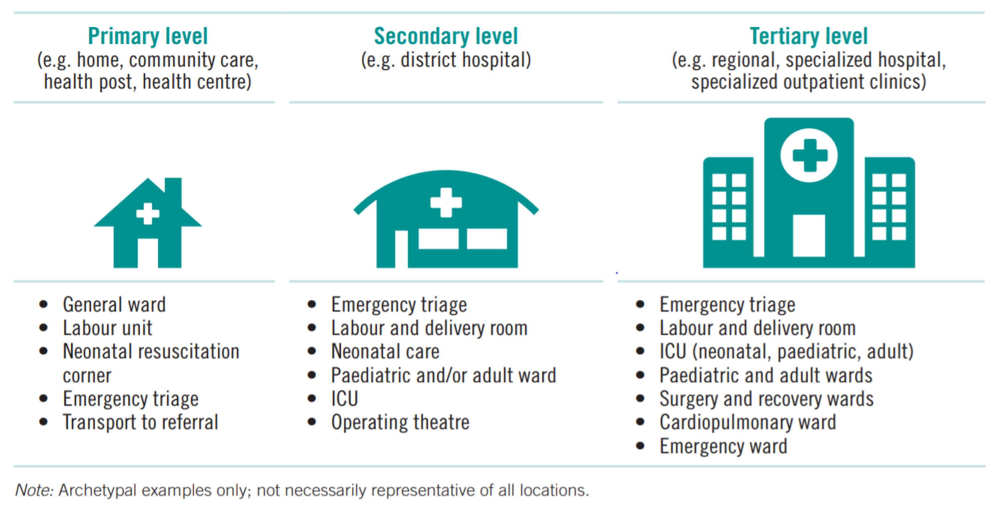
Notably, as identified by Vinson et al. (2006), PSA oxygen-generating plants (based on pressure swing adsorption) are a source of medical-quality O₂ [6]. Therefore, they can serve one of the three levels identified by WHO / UNICEF (see Figure 1). Therefore, this article aims to discuss optimizing oxygen production using PSA oxygen, recognizing the sustained increase in health infrastructure, which generates an increase in oxygen demand in many countries [7,8].

So, we shall compare three different ways to model and optimize the PSA system according to the specifics of a situation. However, to put things in perspective and better evaluate the considerations that we will need to consider in optimizing the process, let us first return to the fundamentals. How do we mainly produce oxygen in the world at the moment?

2. Oxygen Production

While reinforcing that ambient air comprises approximately 78% nitrogen, 21% oxygen, and less than 1% of other gases, oxygen is currently primarily produced in large volumes through the air separation process in industrial air separation units (ASUs). This practice did not change until recently, when oxygen demand in medical use increased substantially, exacerbated notably by the rise of COVID-19. It is now more important than ever to understand the process of extracting oxygen from the air [6].

2.1. Cryogenic Air Separation Unit (ASU)

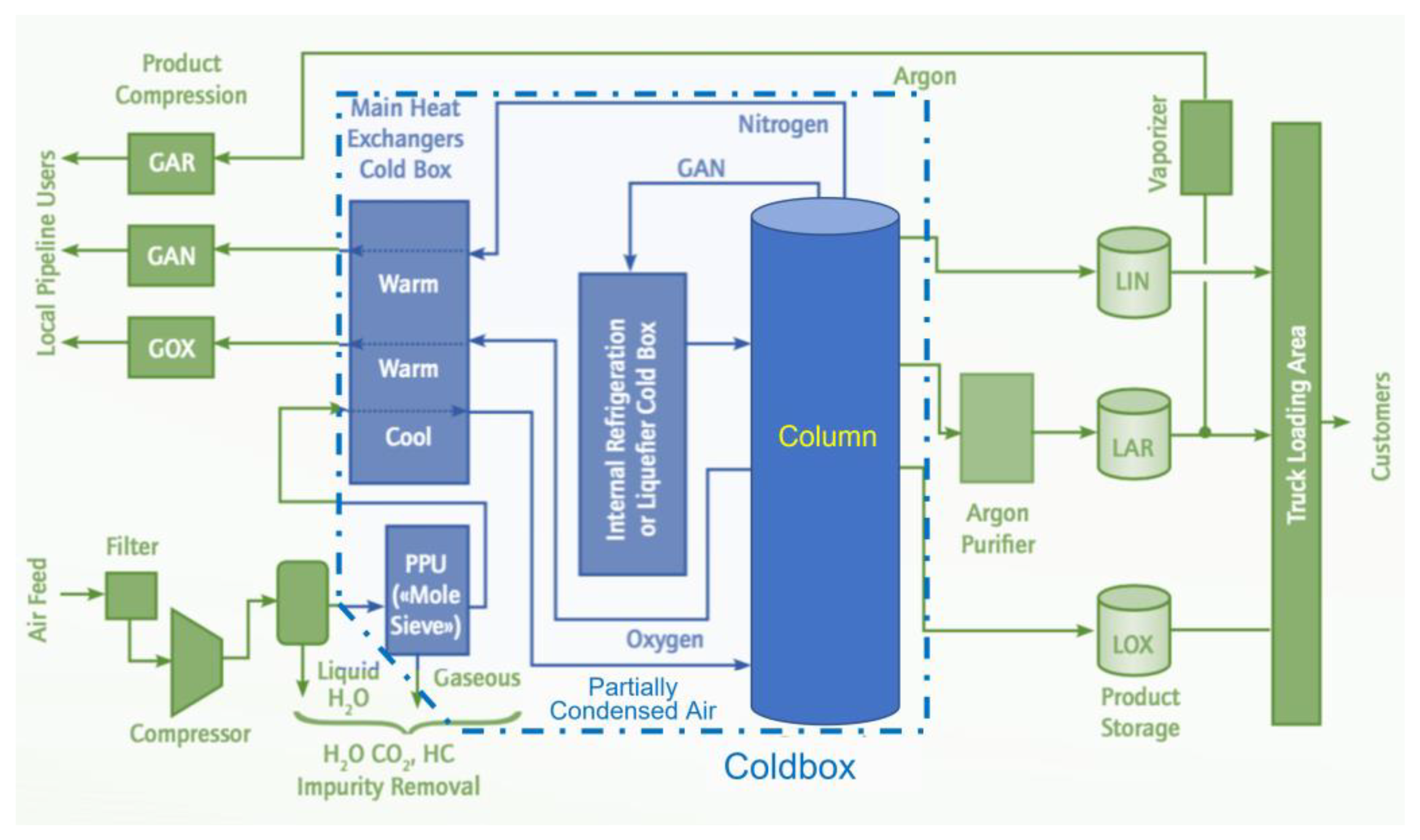
Oxygen produced through the cryogenic process in an ASU can have a very high purity level, up to 99% [9]. The medical use of ASU oxygen is undoubtedly a first when volume justifies the use of this process. This is because, in an ASU, the air goes through a series of processes (see Figure 2). The main items are listed hereafter:

(1)

The air is initially treated in a pre-operation to remove all gross impurities such as hydrocarbons, carbon dioxide, and others.

(2)

The treated air passes through a compressor to be placed under cooling conditions that condense and remove water vapors through a multi-stage process.

(3)

The air is then passed through a molecular sieve absorber that traps the remaining CO₂, H₂O, and hydrocarbons.

(4)

Finally, the (remaining) air enters the distillation columns that fraction (separate) it into its major components, notably nitrogen, oxygen, and argon.

There is a significant difference in the boiling points of each gas; the distillation process works on the basic principle of evaporation of a liquid to separate its components. So, before distillation to convert the gaseous components to liquid form, a cryogenic section is required, hence the name, cryogenic air separation unit [10].

This process is illustrated in Figure 2, which shows a schematic representation of an ASU using the Linde double column approach. As the air rises, the separation process commences. At the bottom of the column, oxygen starts to liquefy. Nitrogen and argon rise as vapors to the column’s top and are collected from the bottom and cooled. The fluid is then fed to the low-pressure column. The objective here is to further distill oxygen, eliminating the remaining argon and nitrogen as much as possible. We now reach 99.5% O₂ purity. Argon is then vaporized, leaving behind liquid oxygen of 99.8% purity. The product can be stored as-is (or heated to ambient room temperature and stored in the gaseous form) [10,11].

2.2. Oxygen Concentrators

For many applications, especially in developing countries with remote areas in poor regions, access to industrial-made medical oxygen is not only more complicated (or expensive), but it is also intermittent and depends on supply chain considerations. So, other means or devices such as an oxygen concentrator that can be used locally are needed. The function of such a device is simply to concentrate oxygen from the ambient air by removing nitrogen through a molecular sieve. Various molecular sieves can be used, but we mostly see ion transport membranes or zeolite. While the process simply uses room air, compresses it, removes nitrogen through the sieve, and finally delivers oxygen, an 85% to 95% purity of oxygen can be generated [6,8].

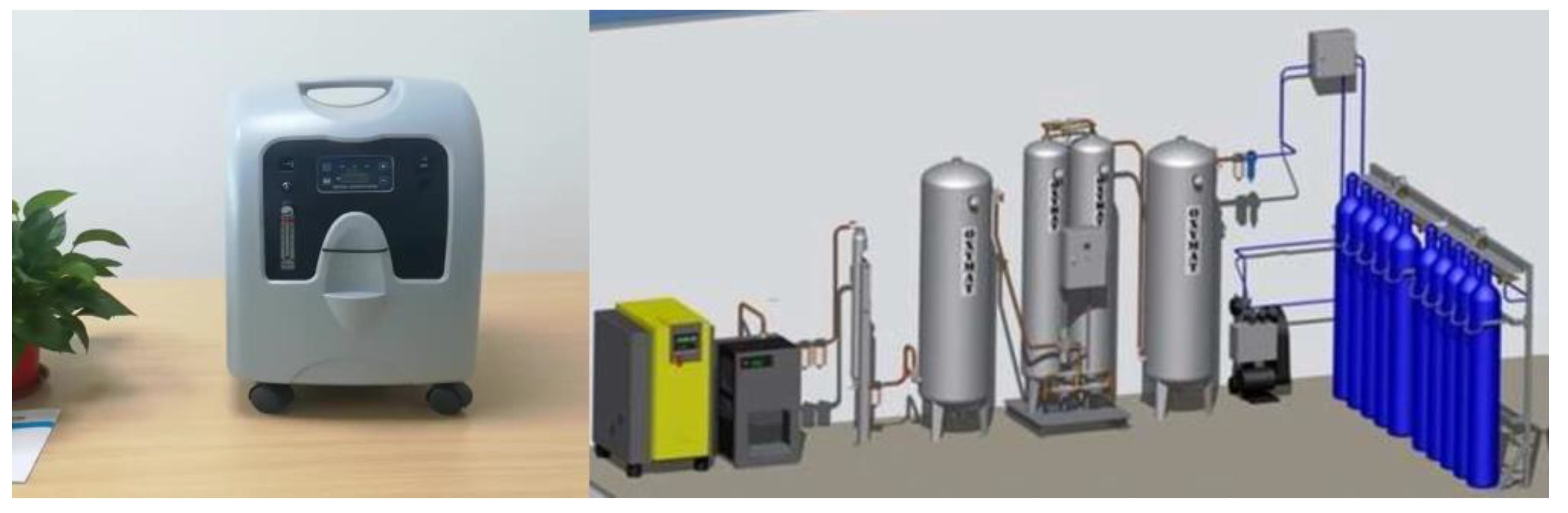
The process’s main challenges and related drawbacks rely principally on the potential malfunctioning of the sieve or an excess of water vapors compromising nitrogen absorption. On the other side, an advantage of the process is that it keeps O₂ delivery independent from the commercial gas producer’s supply [4,7]. Additionally, smaller oxygen concentrator units can be made and even used as portable devices (see Figure 3). Indeed, smaller devices are not the first choice of oxygen delivery system for severe patients, but would instead be a pertinent choice for oxygen therapy at home or in times of crisis, especially for long-term use.

Notably, because of their ease of use (to work, it only needs a continuous electricity supply and room air) and their greater acceptance in the healthcare field, it is even more important for these devices to be optimized from the bigger to the smaller models [3]. Remarkably, some devices produce as low as 0.5–15 L of oxygen per minute, producing medical oxygen from ambient air at small scales.

Medical oxygen concentrators (MOCs) can be used in small- or mid-size-scale oxygen production by using various technologies, but the two most important are pressure swing adsorption (PSA) and membrane technology. This article will focus on the PSA approach, which is more widely recognized and applicable in healthcare settings.

2.3. Pressure Swing Adsorption (PSA) Plant

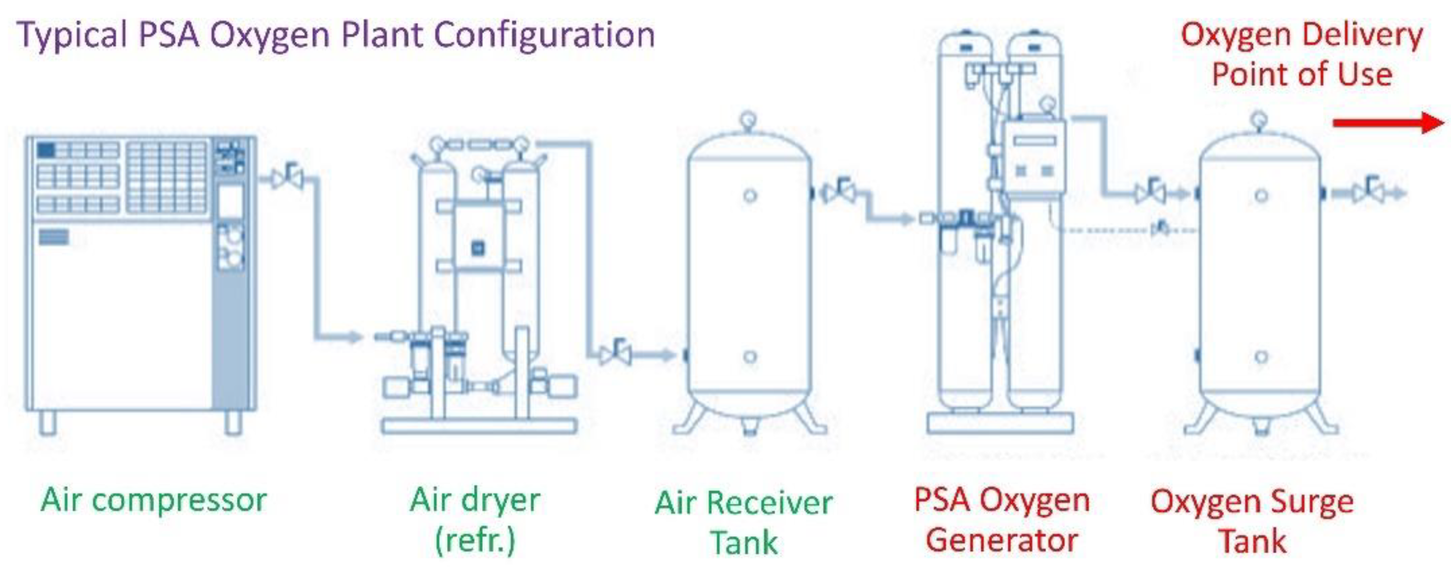
The PSA process operates by pushing the air through a high-pressure container containing an adsorbent bed of zeolite (aluminum-silicates of alkaline metals), which attracts nitrogen more strongly than oxygen. The adsorbent bed absorbs a part of or all the nitrogen. As a result, the gas out of the vessels is richer in oxygen, as shown in Figure 4. Although PSA processes do not produce volumes of oxygen as high as cryogenic plants do, knowledge about their operation is essential because this type of process would likely work around a hospital to meet highly urgent requirements for oxygen in this hospital. PSA plants need an uninterrupted power supply for constant oxygen production [12]. They are dimensioned according to output capacity in cubic meters per hour (m³/h) of oxygen, where 1 m³ = 1000 L of medical oxygen [13].

According to the World Health Organization (WHO) [3], medical-quality oxygen has an O₂ concentration between 90% and 96% (with only N₂ and Ar and remaining). Most adsorption MOCs rely on a PSA process with a selective nitrogen adsorbent to meet this requirement. In addition, small adsorbing particles are used to reduce mass transfer resistance and improve adsorption kinetics. As a result, according to Chai et al. (2011), typical oxygen products obtained from MOC devices consist of 90 to 93% oxygen at a production rate of less than 10 L/min [8].

Due to the limited adsorption capacity of adsorption-based MOCs, the adsorbent is periodically rejuvenated (through regeneration) for effective use [13]. To facilitate a continuous O₂ supply, the product (oxygen) can be collected in an overvoltage column and provided at a certain time, or multiple operations can be used. The configuration of the Skarstrom-type PSA cycle is generally used in MOCs, which consist of stages of production, depressurization, purge, and pressure (see annex A for more details) [14,15]. The quick cycle of the adsorption column maximizes the use of adsorbents and miniaturizes the size of the operation.

Flexibility is also a key feature of PSA since a single MOC unit can be used for many patients with different statuses in a hospital environment. Consequently, optimizing the flexibility and modularity of the PSA process that can quickly shift between different operating regimes to produce oxygen on demand while filling out additional product requirements might be essential. In addition, to meet the need for oxygen varying over time, some are considering a cyber-physical system (CPS) in which the concentration of blood oxygen from a patient with a pulmonary condition is constantly monitored, and actions necessary are taken to modify the functioning of the MOC [15].

There is evidence of the effectiveness of oxygen concentrators in increasing access to life-saving oxygen and improving the overall quality of health care in low-resource settings (LRS). Many studies, including Siew et al. (2012) and Zhu et al. (2017), demonstrated using oxygen concentrators to expand oxygen availability in hospitals in LRS settings [12,14]. These studies have also shown that oxygen concentrators have been successfully used more generally in several developing or emerging countries to provide oxygen in pediatric and surgical departments.

Ultimately, the advantages of MOCs have been discussed in the technical literature; they come with high reliability and low cost compared to oxygen cylinders and piped oxygen systems (Moran et al., 2017) [15]. On the other hand, the disadvantages of PSA-type MOCs include the need for regular, albeit minimal, maintenance and a reliable power supply, which can be addressed by efficient planning and training staff.

3. Observations Related to the Development and Optimization of PSA Units

Some studies have explored interesting innovations in the field of simulation. For example, the mechanisms of heat and mass transfer have been studied and enhanced by Farooq et al. (1989), Teague and Edgar (1999), and Ahari et al. (2006 and 2008) [16,17,18,19].

In particular, the mass transfer rate and the bed pressure drop model were validated with experiments by Farooq and D.M. Ruthven [17] into a summary model of pressure swing adsorption and models adopted to simulate equilibrium separation. The selected adsorbent was zeolite. They also discussed the effects of axial dispersion and mass transfer resistance on system performance. Ahari et al. [19] developed a dynamic model, then set up a lab-scale device to verify accuracy. In their study, they considered the effect of kinetic parameters. They found that more steps for pressure equalization could increase the product recovery rate regarding separation efficiency.

In this work, we focus on PSA processes and analyze some mathematical models of these systems. First, a systematic analysis was implemented including cycle temperature, concentration, and pressure profiles. In addition, several operating parameters such as the duration of each step, the bed H/D (height-to-diameter) ratio, and the flowrate of products were determined to follow these factors’ effects on process performance.

Simulation Challenges

The previous sections illustrate that designing and optimally operating PSA processes can be complex, if not difficult. This is mainly because of the intrinsic non-linear dynamics but is also a consequence of a complex operation with varying operating regimes [20,21]. Consequently, many decision variables must be evaluated, including cycle configuration and operation, pressure levels, purge conditions, and the efficiency of bed regeneration. However, several other objectives must be met for optimal function, including modularity, compactness, reliability, and efficiency.

For example, using the number of tons of oxygen per day (or TPD), the BSF is the amount of adsorbent (in kg ads) required to produce each TPD. Therefore, BSF minimization leads to lower adsorbent inventory levels and smaller MOC units. On the other hand, the oxygen recovery is calculated by calculating the fraction of oxygen recovered at the outlet of the product compared to the quantity of oxygen supplied during a PSA cycle in a cyclic steady state. MOCs are generally small-scale devices with a limited amount of adsorbent and fast cycling [22,23]. However, they may have high power consumption due to frequent pressure changes compared to more significant PSA operations. Nevertheless, the relative ease and dependability of the MOC play a more important role than its power consumption regarding oxygen production (e.g., TPD). While this is especially true for small-scale applications, overall, the main design goals are:

(1)

Increased adsorbent productivity;

(2)

Improved O₂ recovery;

(3)

The development of smaller-size, lower-weight units.

Most of the existing literature mainly focuses on designing PSA-based MOC technologies for fixed product specifications. So, it would be essential to emphasize developing flexible PSA processes that can deal with various end-use oxygen specifications as desirable or simply allowing for purpose changes with a flexible PSA operation to suit different patients’ requirements.

4. Observations and Findings Related to Thermodynamic Analysis of PSA Processes

Even though we might find diverse sources in the literature of the optimization-based process design domain [24,25,26], just a few studies perform flexibility analysis for the operation of complex PSA systems [27,28]. Consequently, we conducted a thermodynamic analysis that could allow for the optimization and what we shall call “operational flexibility” (OF) of PSA-based MOC systems. In this work, we compare three different thermodynamic models:

(1)

A simulation-based optimization framework;

(2)

A first-principles-based model;

(3)

A high-fidelity adsorption simulation model.

While they all rely on NAPDE (non-linear algebraic partial differential equations) modeling, they come with different assumptions and conservation equations that make some of them better suited for some challenges. To make it easier, they are summarized hereafter, noting that some aspects might be simpler to simulate for one model, others might be more difficult, and vice-versa.

To simulate the adsorption processes for air separation operating under a pressure swing, while special consideration according to the specific models will be touched upon in the corresponding sections, we generally consider the process to be based on a Skarstrom-type cycle consisting of a repetition of four different steps:

(1)

The generation of high-pressure products;

(2)

Depressurization;

(3)

A low-pressure purge;

(4)

Pressurization.

We will also touch on decision variables that might apply to the different models. The evaluation and especially the optimization of the PSA process often require optimizing these decision variables (such as cost or size) for minima while satisfying some system requirements.

4.1. Simulation-Based Framework

The first approach that was analyzed is a simulation-based optimization framework. This framework uses a non-linear algebraic partial differential set of coupled equations (PDEs with non-linear terms and constraints that describe mass and energy conservations and transport phenomena through porous media). This non-linear PDE model is complex and difficult to solve, even for fixed conditions [29,30].

In this framework, the cycling series of steps in the PSA process comprise the adsorption (AD), pressure equalization (ED and ER), co-current purge (blowdown) (COD), counter-current purge or blowdown (BD), full purge (PUR), and final pressurization (FR).

Conservation equations:

Mass balance:

$$\begin{gathered} -{\epsilon }_b{D}_{ax,i} {\frac{{\partial }^2{C}_i}{\partial z^2}}^{ }+\frac{{\partial }^2(v_g{C}_i)}{\partial z^2}+\left({\epsilon }_b+\left(1-{\epsilon }_b\right){\epsilon }_p\right)\frac{\partial C_i}{\partial t}+{\rho }_s\left(1-{\epsilon }_b\right)\frac{\partial C_i}{\partial t}=0 \\ {D}_{ax,i}=0.73D_{m,i}+\frac{v_g{r}_p}{{\epsilon }_{b \left(1+9.49 \frac{{\epsilon }_b{D}_{m,i}}{2v_g{r}_p}\right)}} \end{gathered}$$

(1)

Energy balance:

Gas phase:

$$-k_g\frac{{\partial }^2{T}_g}{\partial z^2}+c_{pg}{v}_g{\rho }_g\frac{\partial T_g}{\partial z}+{\epsilon }_b{c}_{vg}{\rho }_g\frac{\partial T_g}{\partial t}+P\frac{\partial v_g}{\partial z}+h_f\left(T_g-T_s\right)+\frac{4h_{wg}}{D_b}\left(T_g-T_w\right)=0$$

(2)

Solid phase:

$$-k_g\frac{{\partial }^2{T}_s}{\partial z^2}+c_{ps}{\rho }_s\frac{\partial T_s}{\partial z}+{\rho }_s{\displaystyle \sum }_{i=1}^n(c_{pg,i}{q}_i)\frac{\partial T_s}{\partial t}+{\rho }_s{\displaystyle \sum }_{i=1}^n\Delta H_i\frac{\partial q_i}{\partial t}-h_f\left(T_g-T_s\right)=0$$

(3)

Bed wall [31]:

$$-k_w\frac{{\partial }^2{T}_w}{\partial z^2}+c_{pw}{\rho }_w\frac{\partial T_w}{\partial z}-h_w\frac{4D_b}{{(D_b+W_t)}^2-D_b{}^2}\left(T_g-T_w\right)+h_{amb}\frac{4(D_b+W_t)}{{(D_b+W_t)}^2-D_b{}^2}\left(T_w-T_{amb}\right)=0$$

(4)

Momentum balance:

$$-\frac{\partial P}{\partial z}=\frac{150\mu {(1-{\epsilon }_b)}^2}{{\epsilon }_b{}^2{(2r_p\mathsf{\Psi })}^2}{v}_g+1.75\frac{\left(1-{\epsilon }_{b\_}\right){\rho }_g}{2r_p\mathsf{\Psi }{\epsilon }_b{}^3}\left|v_g\right|v_g$$

(5)

Adsorption balance:

$$q_i^{*}=\frac{I{P}_{1,i}{e}^{\frac{I{P}_{2,i}}{T}}{P}_i}{1+{\sum }_{i=1}^{n}I{P}_{3,i}{e}^{\frac{I{P}_{4,i}}{T}}{P}_i}$$

(6)

Absorption rate:

$$\begin{gathered} \frac{\partial q_i}{\partial t}=k_{LDF,i}\left(q_i^{*}-q_i\right)=\frac{15D_{e,i}}{r_p{}^2}\left(q_i^{*}-q_i\right) \\ {D}_{e,i}=\frac{{\epsilon }_p}{\tau }\frac{D_{k,i}{D}_{m,i}}{D_{k,i}+D_{m,i}} \\ {D}_{k,i}=97.0 r_p\sqrt{\frac{T}{M_i}} \end{gathered}$$

(7)

For these conservation equations, the following parameters are considered: A_w cross-section area of column wall, C molar concentration of mixture, C_i molar concentrations of component i, c_pg specific heat capacity of gas phase, c_pg specific heat capacity of gas phase, c_ps specific heat capacity of adsorbent, c_pw specific heat capacity of column wall, h_in heat transfer coefficient with inner wall of column, h_out heat transfer coefficient with outer wall of column, Δh_i heat of adsorption of component i, ΔH_i heat of adsorption of component i, k_i mass transfer coefficient of component i, M molar-averaged molecular weight of mixture, M_j molecular weight of component i, n_i dynamic adsorption of component i, n^*_I equilibrium adsorption of component i, n^s_i saturation adsorption of component i, P pressure, q_i dynamic adsorption mass of component i, R universal gas constant, R_in inner radius of column, R_out outer radius of column, t time, T temperature of adsorption bed, T_f ambient temperature, T_w wall temperature, x_i mass fraction of component i y_i, ε_b bed porosity, ρ_g mass concentration (density) of mixture gas, ρ_I mass concentrations of component i, ρ_b bed density of adsorbent, ρ_p particle density of adsorbent, ρ_s skeletal density of adsorbent, ρ_w density of column wall, and Ψ shape factor of the adsorbent particles.

A set of initial conditions and boundary conditions for modeling the adsorption bed used for PSA process simulations is needed (see

Table 2. Initial and boundary conditions of the adsorption bed used for PSA process simulations.

List of Initial Conditions of the Adsorption Bed
	$y_i\left(z\right)=0$, $y_{inert}\left(z\right)=1,$ $q_i\left(z\right)=0, q_{inert}\left(z\right)=q_{eq,inert}\left(z\right),$
	$C_i\left(z\right)=\frac{P{y}_i}{R_{g}T}$, $P\left(z\right)=P_{feed},$ $T_g\left(z\right)=T_s\left(z\right)=T_w\left(z\right)=T_{feed}$
Boundary Conditions for PSA bed simulation
PR (inlet, z = L)
	${\left.\frac{\partial C_i}{\partial z}\right|}_{z=0}=0$
	${\left.u_o\right|}_{z=0}=0$
	${\left.\frac{\partial T_g}{\partial z}\right|}_{z=0}=0$
	${\left.u_{o,inlet}{C}_{inlet,i}\right|}_{z=L}=u_{o}C{C}_p{T}_g-k_g\frac{\partial T_g}{\partial z}$
	${\left.P\right|}_{z=L}=P_{outlet}$
	${\left.u_{o,inlet}{C}_{inlet}{C}_p{T}_{inert}\right|}_{z=L}=u_o{C}_i-{\epsilon }_b{D}_{ax}\frac{\partial y_i}{\partial z}$
AD1, AD2 (inlet, z = 0)
	${\left.u_{o,inlet}{C}_{inlet,i}\right|}_{z=0}=u_o{C}_i-{\epsilon }_b{D}_{ax}\frac{\partial y_i}{\partial z}$
	${\left.u_{o,inlet}{C}_{inlet}\right|}_{z=0}=u_{o}C-{\epsilon }_b{D}_{ax}\frac{\partial y_i}{\partial z}$
	${\left.u_{o,inlet}{C}_{inlet}{C}_p{T}_{inert}\right|}_{z=0}=u_{o}C{C}_p{T}_g-k_g\frac{\partial T_g}{\partial z}$
	${\left.\frac{\partial C_i}{\partial z}\right|}_{z=L}=0$
	${\left.P\right|}_{z=L}=P_{outlet}$
	${\left.\frac{\partial T_g}{\partial z}\right|}_{z=L}=0$
ED1, ED2, ED3, CoD (outlet, z = L)
	${\left.\frac{\partial C_i}{\partial z}\right|}_{z=0}=0$
	${\left.u_o\right|}_{z=0}=0$
	${\left.\frac{\partial C_i}{\partial z}\right|}_{z=L}=0$
	${\left.P\right|}_{z=L}=P_{outlet}$
	${\left.\frac{\partial T_g}{\partial z}\right|}_{z=0}=0$
	${\left.\frac{\partial T_g}{\partial z}\right|}_{z=L}=0$
BD (outlet, z = 0)
	${\left.\frac{\partial C_i}{\partial z}\right|}_{z=0}=0$
	${\left.u_o\right|}_{z=L}=0$
	${\left.\frac{\partial C_i}{\partial z}\right|}_{z=L}=0$
	${\left.P\right|}_{z=0}=P_{outlet}$
	${\left.\frac{\partial T_g}{\partial z}\right|}_{z=0}=0$
	${\left.\frac{\partial T_g}{\partial z}\right|}_{z=L}=0$
ER1, ER2, ER3, PUR (inlet, z = L)
	${\left.u_{o,inlet}{C}_{inlet,i}\right|}_{z=L}=u_o{C}_i-{\epsilon }_b{D}_{ax}\frac{\partial y_i}{\partial z}$
	${\left.u_{o,inlet}{C}_{inlet}\right|}_{z=L}=u_{o}C$
	${\left.u_{o,inlet}{C}_{inlet}{C}_p{T}_{inert}\right|}_{z=0}=u_{o}C{C}_p{T}_g-k_g\frac{\partial T_g}{\partial z}$
	${\left.\frac{\partial C_i}{\partial z}\right|}_{z=0}=0$
	${\left.u_o\right|}_{z=0}=0$
	${\left.\frac{\partial T_g}{\partial z}\right|}_{z=0}=0$
PUR (inlet, z = L)
	${\left.u_{o,inlet}{C}_{inlet,i}\right|}_{z=L}=u_o{C}_i-{\epsilon }_b{D}_{ax}\frac{\partial y_i}{\partial z}$
	${\left.u_{o,inlet}{C}_{inlet}\right|}_{z=L}=u_{o}C$
	${\left.u_{o,inlet}{C}_{inlet}{C}_p{T}_{inert}\right|}_{z=0}=u_{o}C{C}_p{T}_g-k_g\frac{\partial T_g}{\partial z}$
	${\left.\frac{\partial C_i}{\partial z}\right|}_{z=0}=0$
	${\left.P\right|}_{z=L}=P_{outlet}$
	${\left.\frac{\partial T_g}{\partial z}\right|}_{z=0}=0$

). More details concerning the simulation-based optimization model can be found in Bajaj et al. (2018) [30]. One objective for optimizing the MOC unit based on PSA is reduction in the BSF. At the same time, metrics optimization allows for a PSA process with low compression costs, compactness, modularity, and more effective use of adsorbent.

A high apparent density of adsorbent (to adsorb as much N₂ as possible) is preferable. This leads to a greater interstitial fluid velocity, reducing stay in the bed of the incoming ambient air. Moreover, increasing apparent adsorbent density leads to an increase in pressure drop, which could cause an unwanted fall in the product output power pressure. Thus, a higher apparent adsorbent density can lead to the under-use of the packed adsorbent and a reduction in the separation efficiency of the adsorbent. Consequently, it is necessary to balance this “compromise” to define the optimal density of the adsorbent.

While many variables are tied to these boundary conditions, the decision variables can be determined according to the specifics of a design. Additional constraints need to be imposed in this NADPE model to ensure that pressurization, depressurization, and the overall process result in a sufficiently flexible range for purging operations.

4.2. First Principles-Based Modeling

The second version is an adsorption model focused on the first principles approach. In a nutshell, a mathematical model based on first principles (e.g., Glad, 2014 or Bhatt, 2014) defines the physics of adsorption relying on a one-dimensional, diabatic (i.e., non-adiabatic) model but also a non-isothermal and non-isobaric model [32,33]. The model calculates the concentration, temperature, and pressure gradients along the axial length of the column and the time dimension and neglects any variation in the variables for each state along the radial direction (see Figure 5). While this model is based on a different set of assumptions and conservation equations (Arora and Hasan, 2021), it is still based on an NAPDE set of equations; however, it is designed to reduce computational expense [13].

The linear driving force equation (LDF) coupled with Darcy’s law (for a steady-state momentum balance) describes the adsorption kinetics in the model [26]. Experimental data can be fitted (e.g., using Langmuir adsorption isotherms described hereafter) to obtain the adsorption capacity at equilibrium for different conditions and adsorbate species on the adsorbent:

$$q_i^{*}={\displaystyle \sum }_s\frac{m_{i,s}{b}_{i,s}{P}_i}{1+b_{i,s}{P}_i}$$

(8)

where s ∈ {1, 2} are the two adsorption sites, i represents the constituents species, m_i,s is the adsorption capacity for the site (solid phase), and P_i is the partial pressure. In the above equation, b_i,s is computed as follows:

$$b_{i,s}=b_{o,i,s}{e}^{\left(\frac{-\Delta U_{i,s}}{RT}\right)}$$

(9)

where b_o,i,s, and U_i,s are the isotherm fitting parameters.

This set of equations depicts the full thermodynamic approach, which is declined in the mathematical model of the adsorption bed. For such problems, we can use a robust OA, an optimization algorithm, to find the objective functions that result in a maximum (or a minimum) function evaluation. OAs are often using the first and second derivatives of the objective function. The objective and one or more constraints are evaluated using simulations or proprietary codes, up to the point of a gray box problem. When the analytic form of the objective function is unknown, but the analytical form of one or more constraints is known, then such problems are called gray box problems. (Note that optimization problems where the analytic form of the objective function and all the constraints are not available are called black box problems).

The series of assumptions necessary to resolve the thermodynamics calculation according to the process characteristic is listed hereafter:

(1)

Intake (air supply) consists of 21% O₂ and 79% N₂ and is supposed to have an insignificant amount of water and argon.

(2)

The purge and pressurization supply consists of an imposed composition of oxygen and nitrogen.

(3)

A minimum number of cycles (e.g., 50) are simulated to reach a cyclic but steady state, as the output properties are monitored to converge for these many cycles.

(4)

The purge and pressurization supply consists of an imposed composition of O₂ and N₂.

(5)

The lowest achievable pressure is 1 bar.

(6)

PSA cycle steps are limited to a maximum number of four.

(7)

The bed is saturated with air at the first (initial) pressure and supply temperature stage of a PSA cycle.

(8)

The oxygen production stage of the cycle is defined as the first stage, in which air is introduced into the column.

4.2.1. Ideal Gas Constitutive Equation

The ideal gas law is used as the equation of state since it offers good approximation of the behavior of the gas-phase under the considered operating conditions. It is declined it its conventional form:

$$P{y}_i=RT{C}_i$$

(10)

where T is the system temperature, P is the total pressure, y_i, and C_i are the bulk gas-phase mole fraction and concentration of component i, and R is the universal gas constant.

4.2.2. Mass Balances

For the mass balance, we impose the mass flow through the adsorption column to correspond to an ideal plug flow without axial mixing. The mass balance accounts for convection and accumulation in both the gas and solid phase. So, for component i over a differential volume element, it is defined by

$$\frac{\partial (v_g{C}_i)}{\partial z}+{\epsilon }_T\frac{\partial C_i}{\partial t}+{\rho }_B\frac{\partial \overline{q_i}}{\partial t}=0$$

(11)

where t is the time coordinate, v_g is the superficial velocity (of the gas phase), ε_T is the total bed void fraction, ρ_B is the mass of the solid per unit volume of column (or the adsorbent bulk density), and q_i is the particle-average specific concentration of species i in the adsorbed phase (i.e., per unit mass of solid).

4.2.3. Mass Transfer Rate (w/r to LDF)

In a similar way as indicated by Bhatt et al. (2014) [33], the mass transfer coefficient is referred to as MTC, and the linear driving force (LDF) model is used to account for the resistance to mass transfer between the fluid and the porous media, given by

$$\frac{\partial \overline{q_i}}{\partial t}=k_{MT{C}_i}\left(q_i^{*}-\overline{q_i}\right)$$

(12)

where $q_i^{*}$ is the adsorbent loading of component i in equilibrium with the gas-phase composition and kMTC is the lumped, effective MTC, computed by presuming that only the resistances to mass transfer in the fluid film (external) and the macropores are significant:

$$\frac{1}{k_{MT{C}_i}}=\frac{r_P\overline{K_{K,i}}}{3k_{f,i}}=\frac{r_P{}^2\overline{K_{K,i}}}{15{\epsilon }_P{D}_{P,i}}$$

(13)

r_P and ε_P are the radius and porosity of the adsorbent particle (P), respectively.

The macropore diffusion coefficient (DP) is derived from the following equation:

$$D_{\overline{P},i}=\tau \left(D_{\overline{K},i}+D_{\overline{M},i}\right)$$

(14)

K_K,i is the local Henry’s coefficient found using the equilibrium isotherm as:

$$\overline{K_{K,i}}=RT\frac{{\rho }_B}{{\epsilon }_i}\frac{\partial q_i^{*}}{\partial p_i}$$

(15)

where p represents the partial pressure and ε_i is the interstitial (or external) porosity.

To determine the constant molecular diffusion coefficient, DM, from a properties database or similar, τ is the adsorbent tortuosity factor is used. With r_P,mac the macropore radius and M_W,i the molecular weight of the constituent, we can evaluate the Knudsen diffusion coefficient (DK) using the following relationship:

$$D_{K,i}=97.0 r_{p,mac}\sqrt{\frac{\tau }{M_{W,i}}}$$

(16)

Considering that μ_g is the dynamic gas viscosity and ρ_g is the molar gas phase density, the film resistance coefficient k_f;I is calculated from the Schmidt (Sc_i), Reynolds (Re), and Sherwood (Sh_i) numbers using the following set of equations:

$$\begin{gathered} S{c}_i=\frac{{\mu }_g}{D_{M,i}{\rho }_g{M}_W} \\ Re=\frac{\left(3r_P{\rho }_g{M}_W{v}_g\right)}{{\mu }_g} \\ S{h}_i=2+1.1 \sqrt[3]{S{c}_i} \sqrt[5/3]{R{e}_i} \\ {k}_{f,i}=\frac{\left(S{h}_i{D}_{M,i}\right)}{2r_P} \end{gathered}$$

(17)

4.2.4. Linear Momentum Balance

This second model further determines the pressure drop along the axial coordinate, which can be calculated using Ergun’s equation (Ergun, 1952), which is suitable for both laminar and turbulent flows. While the pressure drop estimates depend on the flow direction of the bulk gas during different steps of the process cycle, the (∂P/∂z) depends on many other parameters, including ψ, the shape factor of the adsorbent particles. Therefore, this difference should be considered positive during the pressurization (PR) and purge (PU) steps, while being considered negative during blowdown (BD) and feed (FE).

$$\frac{\partial P}{\partial z}=\pm \left[\mu v_g\frac{0.150{(1-{\epsilon }_i)}^2}{{\epsilon }_i{}^3{(2r_p\mathsf{\Psi })}^2}+1.75\times {10}^{-3}{M}_W{\rho }_g{v}_g{}^2\frac{\left(1-{\epsilon }_i\right)}{2r_p\mathsf{\Psi }{\epsilon }_i{}^3}\right]$$

(18)

4.2.5. Equilibrium Isotherm

In an approach used by Thakur et al. (2011) [34] or Zou et al. (2017) [35], we can determine the adsorption isotherm of the gaseous mixture from pure component isotherms using the well-known extended Langmuir model (EL). This EL is based on modifying the Langmuir prevalent multicomponent adsorption equilibria model centered on single-component isotherms fitted on pure component data. So, the adsorbed moles of component i per unit mass of adsorbent at equilibrium ($q_i^{*}$ are given by:

$$q_i^{*}=\frac{\left(I{P}_{1,i}\right)\left(p_i\right)}{1+{\sum }_{k=1}^2(I{P}_{2,k})(p_k)}$$

(19)

where, as referred to previously, the Langmuir isotherm parameters IP_1,i, and IP_2,i are defined from the pure component i, and p represents the gas partial pressure.

With this second approach, based on modeling the complete cycle of one single bed, the so-called “Single Bed Approach” can retain the accuracy of multiple-bed simulation using the transfer of information through predefined “interaction” modules as soon as the “cross-over” data are accurate enough. As a consequence, the selected scheme significantly improves the computational speed since it reduces the total number of equations to be solved to achieve the final results.

4.3. High-Fidelity Adsorption Simulation Model

Another model consisting of a unidimensional but pseudo-homogeneous, non-isothermal, diabatic, and non-isobaric model represents the third option for modeling. However, it is defined as the high-fidelity model for simulating pressure swing adsorption (PSA) processes. In short, as presented by Haghpanah et al. (2013) [22,36], it is a set of non-linear and algebraic NAPDEs. It is still used to describe species concentration, temperature, and pressure variation along the bed length and time dimension. The first principles equations leveraged in the model are described as follows.

4.3.1. Conservation Equations

The following equation represents the mass conservation of each chemical species i in the gas phase:

$${\epsilon }_t\frac{\partial C_i}{\partial t}={\epsilon }_b\frac{\partial }{\partial z}\left(D_{L}C\frac{\partial y_i}{\partial z}\right)+{\epsilon }_b\frac{\partial \left(v{C}_i\right)}{\partial z}-{\rho }_{b,ads}\frac{\partial \overline{q_i}}{\partial t}$$

(20)

C_i and C are the concentration of component i and total concentration in the gas phase, respectively; y_i is component i gas phase mole fraction; ρ_b,ads is the adsorbent bulk packing density; and ε_b, and ε_t are bed and total void fraction. Moreover, v is the interstitial velocity, q_i is the component i solid phase concentration, DL is the axial dispersion coefficient, and z and t are the space and time dimensions, respectively.

The above component mass balance equation applies the ideal gas law to convert the concentration in terms of gas phase mole fraction, pressure, and temperature. Consequently, the following equation is obtained:

$$\frac{\partial y_i}{\partial t}+\frac{y_i}{P}\frac{\partial P}{\partial t}-\frac{y_i}{T}\frac{\partial T}{\partial t}=D_L\frac{{\epsilon }_b}{{\epsilon }_t}\frac{T}{P}\frac{\partial }{\partial z}\left(\frac{P}{T}\frac{\partial y_i}{\partial z}\right)-\frac{{\epsilon }_b}{{\epsilon }_t}\frac{T}{P}\frac{\partial }{\partial z}\left(\frac{y_{i}vP}{T}\right)-\frac{{\rho }_{b,ads}RT}{{\epsilon }_{t}P}\frac{\partial \overline{q_i}}{\partial t}$$

(21)

where y_i is the component i gas phase mole fraction, P is the gas phase pressure, and T is the gas phase temperature.

The preceding equation represents the constituent mass balance for each chemical species i. To obtain the total mass balance equation, we sum over this equation for all component species i ∈ I. The resulting total mass balance expression is as follows:

$$\frac{\partial P}{\partial t}=\frac{P}{T}\frac{\partial T}{\partial t}-\frac{{\epsilon }_{b}T}{{\epsilon }_t}\frac{\partial }{\partial z}\left(\frac{Pv}{T}\right)-\frac{{\rho }_{b,ads}RT}{{\epsilon }_{t}P}{\displaystyle \sum }_{i\in I}\frac{\partial \overline{q_i}}{\partial t}$$

(22)

For computing the temperature variations due to adsorption and adsorbent–column–wall interactions, the following heat balance equation is utilized along with c_p,ads and c_p,a which are the adsorbent and adsorbate heat capacity (in kJ/kmol), respectively; c_pg is the ideal gas mixture heat capacity (in kJ/kmol); and K_z, the axial heat conductivity:

$$\begin{gathered} \left({\rho }_{b,ads}{c}_{p,ads}+{\rho }_{b,ads}{c}_{p,a}{\displaystyle \sum }_{i\in I}\frac{\partial \overline{q_i}}{\partial t}\right)\frac{\partial T}{\partial t}= \\ {K}_Z\frac{{\partial }^{2}T}{\partial z^2}+\frac{c_{pg}{\epsilon }_b}{R}\frac{\partial \left(vP\right)}{\partial z}-c_{p,a}{\rho }_{b,ads}T{\displaystyle \sum }_{i\in I}\frac{\partial \overline{q_i}}{\partial t}-\frac{c_{pg}{\epsilon }_t}{R}\frac{\partial P}{\partial t} \\ -{\rho }_{b,ads}{\displaystyle \sum }_{i\in I}\frac{\partial \overline{q_i}}{\partial t}-\frac{2h_{in}}{r_{in}}\left(T-T_W\right) \end{gathered}$$

(23)

where ∆Hi is the heat of adsorption of component i_, h_in is the column–wall heat transfer coefficient, and r_in is the bed column radius.

The following steady-state momentum balance, i.e., Darcy’s law, is applied for taking into account the pressure drop along the adsorbent column:

$$-\frac{\partial P}{\partial z}=\frac{150}{4r_p{}^2}{\left(\frac{1-{\epsilon }_b}{{\epsilon }_b}\right)}^2\mu v$$

(24)

where r_p is the particle radius and µ is the gas mixture viscosity.

The linear driving force (LDF) model uses ∂q_i to reduce the computational complexity of capturing the mass transfer of adsorbate from gas to the solid phase and vice versa,

$$\frac{\partial \overline{q_i}}{\partial t}=k_i\left(q_i^{*}-\overline{q_i}\right)$$

(25)

where $q_i^{*}$ is the equilibrium adsorption capacity computed using a dual-site Langmuir isotherm and k_i is the LDF mass transfer coefficient.

4.3.2. MOC Process Performance Metrics

With the high-fidelity model, the oxygen purity (PO2) is obtained for the production stage of the PSA process by determining the amount of O₂ at the product exhaust divided by the total amount of O₂ and N₂ as follows:

$$P_{O_2}=\frac{\left({\left.{{\displaystyle \int }}_0^{tf}\frac{y_{O_2}\overline{P}\overline{v}}{R\overline{T}}\frac{P_0{v}_0}{T_0}\right|}_{z=1}dt\right)}{\left({\left.{{\displaystyle \int }}_0^{tf}\frac{y_{O_2}\overline{P}\overline{v}}{R\overline{T}}\frac{P_0{v}_0}{T_0}\right|}_{z=1}dt\right)\left({\left.{{\displaystyle \int }}_0^{tf}\frac{y_{N_2}\overline{P}\overline{v}}{R\overline{T}}\frac{P_0{v}_0}{T_0}\right|}_{z=1}dt\right)}$$

(26)

where Z = 1 denotes the product outlet end, y_O2 and y_N2 are the gas phase compositions of oxygen and nitrogen; P, v, and T are the scaled pressure, interstitial velocity, and temperature, respectively; P₀, v_0, and T₀ are the respective scaling parameters; and t_f is the production step duration of a cycle [37,38].

The net oxygen output amount is calculated by subtracting the amount of oxygen utilized during the purge and pressurization stages from the amount of oxygen obtained during the production stage. As a result, the overall O₂ recovery (R_O2) of a PSA cycle is derived as follows, wherein the denominator represents the amount of fresh oxygen fed during the production step:

$$R_{O_2}=\frac{\left({\left.{{\displaystyle \int }}_0^{tf}\frac{y_{O_2}\overline{P}\overline{v}}{R\overline{T}}\frac{P_0{v}_0}{T_0}\right|}_{z=1}dt\right)-\left(\frac{y_{p,O_2}{P}_p{v}_p{t}_p}{R{T}_p}\right)-\left({\left.{{\displaystyle \int }}_0^{t_{pres}}\frac{y_{pres,O_2}\overline{P}\overline{v}}{R{T}_{pres}}\frac{P_0{v}_0}{T_0}\right|}_{z=pres,inlet}dt\right)}{\left(\frac{y_{f,O_2}{P}_f{v}_f{t}_f}{R{T}_f}\right)}$$

(27)

where y_p,O2, y_pres,O2, and y_f,O2 are the oxygen molar fractions of the purge, pressurization, and production feed streams and T_p, T_f, and T_pres are the purge, production, and pressurization step feed temperatures. T_p and t_f are the duration for the purge and production steps, and Z = pres.inlet at the inlet column end during the pressurization step. In addition, v_p, v_f, P_p, P_f are the interstitial feed velocity and pressure for the purge and production streams.

The net number of moles of oxygen collected during production is converted to L/min in standard conditions to calculate the standard amount of oxygen production rate (PC_O2) as follows:

$$P{C}_{O_2}=\left[\left({\left.{{\displaystyle \int }}_0^{tf}\frac{y_{O_2}\overline{P}\overline{v}}{R\overline{T}}\frac{P_0{v}_0}{T_0}\right|}_{z=1}dt\right)-\left(\frac{y_{p,O_2}{P}_p{v}_p{t}_p}{R{T}_p}\right)-\left({\left.{{\displaystyle \int }}_0^{t_{pres}}\frac{y_{pres,O_2}\overline{P}\overline{v}}{R{T}_{pres}}\frac{P_0{v}_0}{T_0}\right|}_{z=pres,inlet}dt\right)\right]\left(\frac{R{T}^{ST P} \times 1000 \times 60}{p^{ST P}{t}_{cycle}}\right)$$

(28)

where T^STP = 273 K and P^STP = 101,325 Pa are the standard temperature and pressure conditions, and t_cycle is the duration of a PSA cycle in seconds.

Finally, we compute the BSF in terms of the quantity of adsorbent required in kg to generate 1 ton per day of net O₂ product as follows:

$$BSF=\frac{{\rho }_{b,ads}\pi r_{in}^{2}L}{\left[\left({\left.{{\displaystyle \int }}_0^{tf}\frac{y_{O_2}\overline{P}\overline{v}}{R\overline{T}}\frac{P_0{v}_0}{T_0}\right|}_{z=1}dt\right)-\left(\frac{y_{p,O_2}{P}_p{v}_p{t}_p}{R{T}_p}\right)-\left({\left.{{\displaystyle \int }}_0^{t_{pres}}\frac{y_{pres,O_2}\overline{P}\overline{v}}{R{T}_{pres}}\frac{P_0{v}_0}{T_0}\right|}_{z=pres.inlet}dt\right)\right]}\left(\frac{1000 \times t_{cycle}}{24 \times 3600 \times 0.032}\right)$$

(29)

where ρ_b,ads is the adsorbent bulk density, and r_in and L are the column radius and length, respectively.

4.4. Benchmarking Numerical Data and Modeling Output

The three studied models were benchmarked according to experiments in different studies. To add more context to this benchmarking and its importance on the performance and operating conditions see Ref. [39] or find more information on the PSA design, the conservation equations, and the assumptions can be found in the Supporting information (see Appendices: (A) The Principle of Pressure Swing Adsorption; (B) Assumptions and conservation equations; (C) Other design considerations; (D) Examples of variables Bounds for Process Optimization.) In the appendices, Figure S1 illustrates the PSA-based MOC cycle divided into its eight processes, while Figure S2 shows the PSA (Skarstrom-type cycle) generic process. Tables S1, S2 and S3 respectively give examples of Operating conditions and performance, Decision variable bounds on design and operation, and Parameters utilized for solving the NAPDE-based process simulation.

Table 3. Experimental data used to benchmark the 3 models under specific operating condition compared in terms of BSF, purity, and recovery.

Model	Pa	Pd	Cycle	Cycle	Purity	Recovery	Flowrate	BSF	Ref.
	(kPa)	(kPa)	Type	Duration (s)	(%)	(%)	(LPM)	(kg ads/TPD)
(1) S-BOF	240	60	5-step	7	90	29.5	0.75	82.8	[12]
(1) S-BOF	355	101	2-step	1.32	90	10–55	5	–	[30]
(1) S-BOF	300	100	4-step	18	94.5	21.3	3.7	–	[40]
(1) S-BOF	300	100	6-step	16	94.5	34.1	4.3	–	[40]
(2) F-P-BM	150	101	4-step	100	93.4	20.1	0.07	–	[17]
(2) F-P-BM	400	100	4-step	3 to 9	90	15–30	1–3	45–70	[34]
(2) F-P-BM	253	101	6-step	5	92	30	1	78	[29]
(3) H-FASM	195	43	6-step	3.8 to 6.8	92–93	41–45	–	23.1–36.7	[15]
(3) H-FASM	304 to	101	4-step	3 to 5	90	25–35	5	11.3–22.7	[8]
	405
(1) S-BOF: Simulation-based optimization framework,
(2) F-P-BM: First-principle-based modeling
(3) H-FASM: High-fidelity adsorption simulation Model. Fitting Parameters: Operating pressure: adsorption Pa and desorption Pd (kPa) Cycle duration of the PSA process tcycle: (s) Oxygen purity (%) Oxygen recovery (%) Production flowrate (LPM) BSF: Amount of adsorbent required in kg to generate 1 ton per day of net O2 product (kg ads/TPD)

compares the process and performance metrics for many reviewed studies. Experimental data used to benchmark the three models under specific operating conditions were compared in terms of BSF as defined in Equation (29), as well as purity and recovery %. Notably, [12] devised a rapid PVSA process with intermediate pressurization steps using Li⋅LS⋅X zeolite and observed that lower desorption pressure levels contributed to lowering BSF and increasing oxygen recovery. Their test unit produced 90% pure oxygen at 0.75 L/min with a BSF of 82.8 kg ads. O₂/TPD with an oxygen recovery of 29.5%. Ref. [40] performed simulation and optimization studies for studying four-step PSA and PVSA cycles for oxygen production with three different candidate adsorbents. Out of Sylobead MS S624, Oxysiv5, and Oxysiv7, Oxysiv7 showed the best separation performance for both PSA and PVSA cycles with 94.5% oxygen purity, 21.3% recovery and a 3.7 L/min production rate. The authors extended their analysis to investigate a six-step PSA cycle for small-scale medical applications and obtained a 94.5% pure oxygen product with 34.1% recovery and a 4.3 L/min production rate. Ref [17] carried out simulation and experimental studies to investigate a two-bed four-step PSA process for air separation using 5A zeolite. The theoretical results confirm that an oxygen product with 93.4% purity can be obtained, notwithstanding a low oxygen recovery of 20.1% and a low production rate of 0.07 L/min. Ref [30] proposed a two-step pulsed PSA process to extend the potential miniaturization for medical applications. With alternating pressurization and depressurization steps, they were able to achieve an oxygen purity of 90% at a production rate of 5 L/min using 5A and Ag⋅Li⋅X zeolite adsorbents. The authors of [34] elaborated a four-step rapid PSA process that produces a 90% oxygen product at 1–3 L/min with an oxygen recovery of 15–30% and BSF of 45–70. Ref. [29] developed a four-bed rotary value rapid PSA process to enhance air separation performance. The results indicate that a 92% O₂ purity at 1 L/min production can be achieved with an oxygen recovery of 30% and a BSF of 78. Finally, [8] developed a rapid PSA process using Li⋅X zeolite with a total cycle time in the range of 3–5 s. They were able to obtain 90% pure oxygen product with 25–35% recovery with a BSF of 11.3–26.7 kg ads. O₂/TPD. Overall, all three models show good correspondence with experimental data with ±5 to 10% accuracy.

5. Discussions

While we have discussed various systems, we acknowledged that large-scale methods (such as cryogenic fractionation units) are unsuitable for medical institutions because of their substantial investment and large occupation of area [39]. So, we emphasized the continued research need for optimizing and miniaturizing smaller oxygen PSA plants. This is not only of practical significance, but it is also relevant to progress towards compact equipment and a high degree of automation.

To ensure the flexibility of the PSA, the question lies in over-designing the apparatus to deliver a higher purity of oxygen than desired at a determined minimal flow rate. After that, we resolve to obtain PSA size and operating conditions while maximizing the mapping of the possible use specifications (e.g., we can do so by determining the area covered by flow rate and purity). Consequently, as soon as there becomes a need for greater throughput or purity, such an adaptable PSA process could take on new product specification requirements with flat (or fixed) output equipment without breaching the request for purity. Therefore, we only need to model a single bed for continuous oxygen delivery instead of completely modeling a multiple-beds configuration.

5.1. Modeling Considerations

We investigated ways to optimize portable medical oxygen concentrators (MOCs) using the PSA process to generate and deliver medical-grade O_2, notably for patients with serious lung diseases, COVID-19 or COPD. In particular, we can model or optimize flexible adsorption PSA-based apparatuses able to produce O₂ with variable flow rates and purity requirements over time. In addition, the flexible design is inherently advantageous because the same device can be adapted to meet changing oxygen needs.

So, all decision criteria need to be considered, not just in the purely thermodynamic-related aspect but also the cost, size, and functionality aspects. Vice-versa, taking care only with cost and ease of installation does not optimize the quality of the generated oxygen. In addition, one can add the following contextual operating conditions for oxygen therapy, which should be adjusted appropriately based on the assessment of oxygen requirements (see WHO, 2020, 2021).

5.1.1. Maximum Flow Output

O₂ needs evaluation to characterize the upper limit flow a MOC should deliver. Small MOCs are often available as 3 to 10 LPM units. As an example, while children take at most 2 LPM, a 5 LPM device could simultaneously support two pediatric patients (even if one is with hypoxic acute respiratory illness). On top of that, this 5 LPM unit could help adults. Based on current WHO guidelines [3]: “An oxygen concentrator unit that delivers between 1 and 10 LPM would be the most versatile for surgical care applications.”.

5.1.2. Oxygen Concentration Output at Higher Altitudes

One of the considerations that receive more importance while supply chains are stretched and often unable to appropriately respond to the demand for medical oxygen is higher altitude (being scarcer in oxygen, e.g., oxygen levels from sea level at 20.9% O₂ become 19.4% at 2000 m or even 18.6% at 3000 m). Although partial (O₂) pressure in the atmosphere is smaller at high altitudes, patients in the installations of these higher altitudes may require higher volumetric flowrates for adequate medical oxygen quality than patients at sea level, this being especially true for longer duration therapy. Beyond 2000 m (above sea level), the performance requirements of devices at high temperatures and humidity should not be as strict as those provided in early studies since the conditions rarely reach up to extremes (i.e., 313 K and 95% RH simultaneously) at these altitudes because temperature and humidity tend to decrease at higher altitudes [5]. Since two parameters play opposite directions, modeling might be the only way to define a design’s final outcome or optimum.

5.1.3. Humidification

While it is always key to refer to clinical guidelines to decide if adding humidity to medical gas, per WHO standards, is not required when O₂ is utilized at minimal flow rates (i.e., less than 2 L per minute), nonetheless, it may be necessary for higher O₂ flowrate needs. In this case, a special bottle (for example, for humidification) might be connected between the MOC and the patient (i.e., in the breathing circuit). Humidifiers typically have threads for direct attachment to concentrators with threaded outputs or require a humidifier adapter for concentrators with oxygen-barbed connectors.

5.1.4. Recommendations

Our recommendations are two-fold, and they are tied to the ultimate goal of the modeling process:

• First, we suggest considering a simulation-based optimization framework (see Section 4.1) or high-fidelity modeling (see Section 4.3) to cope with the optimization-related challenges with varying specifications and operations and to achieve this with higher accuracy. These two would allow for the best synthesis (design + operation) of adsorption-based MOC systems but also require more computation time and resources.
• Second, the simpler first-principles-based model (see Section 4.2), with simplifications and assumptions, makes it faster to generate a large volume of scenarios and, in that way, could represent a better approach for a feasibility study dealing with many options and designs. So, it would be the first choice for a quick turnaround process evaluation, establishing a diversity of scenarios, or unfolding feasibility studies.

5.2. Cost Effectiveness

One aspect of this discussion is the operating costs of a MOC. For a PSA oxygen plant to be cost-effective and feasible for quick implementation, especially in remote locations, proper modeling of its implementation should be performed. So, time is essential for the PSA plant to stay relevant and cost-effective. Therefore, modeling should be kept fast and reliable. Especially in periods of emergency, a well-designed PSA process would be a more feasible option, although it should be reserved for mid-size or small-size installations, since it is more expensive for larger volumes of pure O₂.

Notably, there is convincing evidence that well-designed PSA-based units are a feasible and cost-effective approach for administering O₂ therapy, notably where oxygen cylinders and piped systems are unsuitable or inaccessible (Duke et al. 2010, WHO 2020) [2,7]. This relies on high-quality MOCs that can provide multiple patients with a viable but flexible and reliable source of O₂. While oxygen concentrators draw from the ambient air to deliver constant, clean, and highly-concentrated O₂, MOCs may operate for multiple years (e.g., up to five years) with minimal energy supply, maintenance, and upkeep needs. Therefore, it is important to have them properly designed, if not optimized, to support a mix of potential situations.

An exergy analysis in order to validate the conclusion is prominently featured in

Table 4. Variation in the operating pressure, compressor work, and energy consumption with feed purity for MOCs at an operating temperature of 333 K.

Mole Fraction of Oxygen in Feed	Pressure	Compressor Work (Wc)	Energy Consumption per O2 Nm3
	kPa	(kJ/mol)	(kWh)	(kJ)
0.21	390	41,120	0.509	1832
0.40	290	23,620	0.293	1055
0.50	250	18,430	0.228	821
0.60	220	14,600	0.181	652
0.70	190	11,640	0.144	518

. This exergy analysis allows us to compare different processes based on the second law of thermodynamics by finding the exergy loss in the process units. Exergy analysis represents a fundamental tool for the optimization of a process, individuating the unit equipment characterized by lower exergy efficiency. The exergy of the process can be evaluated by the following equation:

$$Exin/out=Min/out\left[\left(H-H0\right)-T0\left(S-S0\right)\right]$$

(30)

where M [kmol/s] is the molar flowrate of the studied stream entering the unit equipment, H is the molar enthalpy at P and T, H0 is the molar enthalpy at the pressure and temperature of the equilibrium state (i.e., P = 1 atm and T = To = 298 K), S is the entropy at P and T, and So is the entropy of the stream under equilibrium state conditions. Both molar enthalpies are in [kJ/kmol], while the entropies are in [kJ/K⋅kmol].

The chemical exergy in the PSA section of the process is calculated as:

$$Exin/out=Min/out\left(\mathsf{\Sigma }n i xi exi+RTo \mathsf{\Sigma }ni xi \ln \left(xi\right)\right)$$

(31)

where n is the number of chemical species, xi is the mole fraction of i species at inlet or outlet, exi (kJ/kmol) is the standard chemical exergy of i species at P = 1 atm and To = 298 K, and R is the gas constant.

The exergy associated with mechanical processes, such as fluid machinery (e.g., pumps and compressors), is equal to the unit power, whereas the exergy related with a heat transfer can be calculated using the Carnot efficiency. Note that the kinetic and potential exergy are neglected since their order of magnitude is much lower than the chemical and process exergy contributions. Table 4 and

Table 5. Impact of operating conditions on power consumption and lost work (exergy destruction) for MOCs.

Input Temperature (K)	N2 Equilibrium Constant	O2 Equilibrium Constant	Operating Pressure	Compressor Work (Wc)	Lost Work (Destroyed Ex) in PSA	MOC Typical Power Consumption
						5 LPM	10 LPM	20 LPM
			(kPa)	(kJ/kmol)	(kJ/kmol)	(W)	(W)	(W)
303	9.94	5.40	390	41,120	13,430	153	305	611
318	8.24	4.50	380	40,080	12,940	149	298	595
333	7.55	3.72	420	44,490	14,980	165	330	661
293	5.98	2.56	460	48,880	16,960	182	363	726

show the impact of operating conditions on the main parameters involved in the exergy analysis. Table 4 outlines the impact of varying mole faction of oxygen in the feed, while Table 5 put forward the input temperature influence on Typical power consumption for different size of MOC.

The exergy efficiency and destroyed exergy are calculated:

$$\eta =\frac{Exprod}{ Exfeed }=1-\frac{Extot d}{ Exfeed }$$

(32)

$$Extot d=Exfeed-Exprod=T_{AMB} Sgen$$

(33)

where Exprod and Exfeed are the total exergy produced from the system and the input (i.e., fed to the system), respectively, T_AMB is the ambient temperature, and Sgen is the entropy generated (in [kJ/K⋅kmol]). The destroyed exergy might then be divided into exergy lost to irreversibility and waste. Figure 6 illustrates, with a “Grassman” diagram, the flow of exergy in the system for operation at 390 kPa operating conditions (numbers in % of Input exergy or Exfeed).

Table 6. Typical calculation of backup energy requirement for MOCs.

Variable	Notes	Example Value
(A) MOC consumption [power in W]	Usually, 100 W and 600 W for small units, contingent on the operating conditions and sizes	600 W (Corresponding to a 20 LPM unit approximately—see exergy analysis)
(B) The approximate duration of a typical power outage to support [average in hours per day]	Varies from facility to facility	3 h
(C) Additional compensation for losses [% relating to a reasonable reserve according to the context]	Consider that electric energy storage (such as Li batteries) will lose capacity and necessitate replacement over time	10%
(D) Battery depth-of-discharge	10–70% depending on the battery type	40%
Sample calculations
(E) Total concentrator backup energy requirement per day	A × B × (1 + C)	600 W × 3 h × (1 + 0.10) = 1980 Wh = 1.98 kWh
Total backup (electrical battery) energy storage requirements	E × (1/D)	1980 Wh × (1/0.4) = 3960 Wh = 4.95 kWh

Note: the total energy stored in a battery bank (in Wh) is equal to the total number of batteries × V × Ah. (Ah, ampere hour; kWh, kilowatt hour; Wh, watt hour).

illustrates the extent of the simulation conditions and some of the outcomes of the complementary exergy and energy-related simulation by showing a typical calculation of the backup energy requirement for a MOC.

5.3. New Avenues

While we have focused primarily on optimizing the performance of flexible PSA processes and defining the feasibility area of product specifications (output), the outcomes can be easily expanded to innovative approaches and procedures. For example, with simpler/faster simulation schemes, we could even imagine using such an adaptable PSA device in a monitored environment (in which patients are continuously supervised for the rate of change in the oxygen level in their blood) such that a microcontroller validates the optimal control action policies to reconfigure the operation of the MOC to meet the patient’s oxygen needs in real time. This microcontroller (with or without artificial intelligence) can routinely reconfigure the MOC function in real time to meet different product (or therapy) requirements. Importantly, any optimization modeling discussed here quickly shows how variations in required O₂ flow and purity can be accommodated with the use of flexible MOCs. Even though a PSA unit is 0intended for assumed flow and purity levels, the controller can make appropriate operating modifications to achieve a patient’s oxygen specification requirements. The exergy analysis performed and reported in Section 5.2 outlines the potential for improvements in the process in reducing the exergy destroyed at the compressor level, in the PSA process and in waste stream management (see Figure 6).

However, real-time O₂ demand distribution requires developing a high-fidelity microcontroller with a fast feedback time, a topic for another discussion. To make it effective and accurate, the way forward would be an efficient translation into machine learning models or even deep learning networks that might be better suited to simulate the complex PSA process. Artificial intelligence might be needed to aim beyond the prediction of such a dynamic process outcome to implement real-time adjustments of these outcomes.

6. Conclusions

The underlying research and this review of modeling approaches represent an attempt to add to the undertaking of providing support for important medical devices. We benchmarked three thermodynamic simulation models of the PSA process for medical oxygen generation. The intent was for the analysis to unveil to what extent these models could allow for the optimization and operational flexibility of PSA-based MOC systems. It is well known that medical PSA oxygen generator plants can be a source of medical-grade oxygen. However, they need to be designed accordingly and properly operated. Amongst the key optimization goals (or criteria) of improving or modeling MOCs, we can identify the following:

(1)

Enhancing adsorbent productivity;

(2)

Increasing O₂ recovery;

(3)

Improving unit compactness and weight.

These specific criteria become even more important with adsorbents with high-level selectivity (N₂/O₂), efficient cyclic procedures, and PSA-based devices. Furthermore, optimization is even more important since these technologies have already undertaken substantial reductions in CAPEX and OPEX (i.e., capital and operating expenditures). This makes them more and more viable (per production unit) compared with cryogenic ASUs. However, further modeling and optimization are required to implement adaptable systems in specific and varying contexts, such as remote locations, energy-limited regions, and low-resource areas.

Considering the issues with undertaking optimization of the PSA process and its adaptable management, we suggest both a “simulation-based optimization framework” (Section 4.1) and a “high-fidelity modeling” (Section 4.3). However, the simpler “First-Principles-based model” (Section 4.2), with simplifications and assumptions, makes it faster to generate a large volume of scenarios and, in that way, could represent a better approach for a feasibility study dealing with many options and designs.

While we focused on optimizing MOC process performance, the analysis quickly illustrates the possibilities, including innovative approaches. One example is to use flexible PSA-based MOCs in the monitored environment to determine MOC optimal control to meet the patient’s oxygen requirements in real-time. The effects of design and operating conditions shall be mapped to help the designers and engineers map outlet product specifications and production effectiveness. To make it practical and accurate, the way forward would be an efficient translation into machine learning models or even deep learning networks that might be better suited to simulate the complex PSA process. Continuing research is needed, and additional steps might include obtaining faster and more accurate real-time modeling and integrating artificial intelligence into the mix.

As a concluding remark, PSA plants can be turn-key units when properly optimized, e.g., using any of the three tools discussed in this article. However, optimization is not the only required item in implementing a PSA O2 plant. For example, the operating staff are critical, and maintaining them requires specialized training. In addition, strict maintenance schedules are needed to prevent malfunctions, while a reliable supply chain is required to meet any additional needs.

References

- Cabello, J.B.; Burls, A.; Emparanza, J.I. Oxygen therapy for acute myocardial infarction. Cochrane Database Syst. Rev. 2010, 128, 641–643. Available online: https://www.cochranelibrary.com/cdsr/doi/10.1002/14651858.CD007160.pub4/full (accessed on 10 February 2023).
- WHO. WHO-UNICEF Technical Specifications and Guidance for Oxygen Therapy Devices; WHO Medical Device Technical Series; World Health Organization and the United Nations Children’s Fund (UNICEF): New York, NY, USA, 2019; ISBN 978-92-4-151691-4. Available online: https://www.who.int/publications/i/item/9789241516914 (accessed on 15 March 2023).
- Vo, D.; Cherian, M.N.; Bianchi, S.; Noël, L.; Lundeg, G.; Taqdeer, A.; Jargo, B.T.; Okello-Nyeko, M.; Kahandaliyanage, A.; Setumbwe-Mugisa, O.; et al. Anesthesia capacity in 22 low and middle income countries. J. Anesth. Clin. Res. 2012, 3, 207. Available online: https://www.mendeley.com/catalogue/e5655211-eaf0-3a74-b636-33bf7e144931/ (accessed on 15 March 2023).
- Kobayashi, N.; Shinagawa, S.; Nagata, T.; Shimada, K.; Shibata, N.; Ohnuma, T.; Kasanuki, K.; Arai, H.; Yamada, H.; Nakayama, K.; et al. Usefulness of DNA Methylation Levels in COASY and SPINT1 Gene Promoter Regions as Biomarkers in Diagnosis of Alzheimer’s Disease and Amnestic Mild Cognitive Impairment. PLoS ONE 2016, 11, e0168816. [Google Scholar] [CrossRef] [PubMed] [Green Version]
- WHO. World Health Organization Oxygen Sources and Distribution for COVID-19 Treatment Centres. 2020. Available online: https://www.who.int/publications/i/item/oxygen-sources-and-distribution-for-covid-19-treatment-centres (accessed on 15 March 2023).
- Vinson, D.R. Air separation control technology. Comput. Chem. Eng. 2006, 30, 1436–1446. [Google Scholar] [CrossRef]
- Duke, T.; Graham, S.M.; Cherian, M.N.; Ginsburg, A.S.; English, M.; Howie, S.; Peel, D.; Enarson, P.M.; Wilson, I.H.; Were, W.; et al. Oxygen is an essential medicine: A call for international action. Int. J. Tuberc. Lung Dis. 2010, 14, 1362–1368. Available online: https://pubmed.ncbi.nlm.nih.gov/20937173/ (accessed on 15 March 2023).
- Chai, S.W.; Kothare, M.V.; Sircar, S. Rapid Pressure Swing Adsorption for Reduction of Bed Size Factor of a Medical Oxygen Concentrator. Ind. Eng. Chem. Res. 2011, 50, 8703–8710. Available online: https://pubs.acs.org/doi/pdf/10.1021/ie2005093 (accessed on 21 March 2023). [CrossRef]
- Bucsa, S.; Serban, A.; Balan, M.C.; Ionita, C.; Nastase, G.; Dobre, C.; Dobrovicescu, A. Exergetic Analysis of a Cryogenic Air Separation Unit. Entropy 2022, 24, 272. [Google Scholar] [CrossRef]
- Huo, C.; Sun, J.; Song, P. Energy, exergy and economic analyses of an optimal use of cryogenic liquid turbine expander in air separation units. Chem. Eng. Res. Des. 2023, 189, 194–209. [Google Scholar] [CrossRef]
- Hamayun, M.H.; Ramzan, N.; Hussain, M.; Faheem, M. Evaluation of Two-Column Air Separation Processes Based on Exergy Analysis. Energies 2020, 13, 6361. [Google Scholar] [CrossRef]
- Zhu, X.; Liu, Y.; Yang, X.; Liu, W. Study of a novel rapid vacuum pressure swing adsorption process with intermediate gas pressurization for producing oxygen. Adsorption 2017, 23, 175–184. Available online: https://link.springer.com/article/10.1007/s10450-016-9843-4 (accessed on 15 March 2023). [CrossRef]
- Arora, A.; Hasan, M.M.F. Flexible oxygen concentrators for medical applications. Sci. Rep. 2021, 11, 14317. [Google Scholar] [CrossRef]
- Siew-Wah, C.; Sircar, S.; Kothare, M.V. Miniature Oxygen Concentrators and Methods. US Patent 8,226,745, 24 July 2012. Available online: https://jhu.pure.elsevier.com/en/publications/feasibility-study-of-miniature-oxygen-concentrator-via-pressure-s-3 (accessed on 21 March 2023).
- Moran, A.; Talu, O. Role of pressure drop on rapid pressure swing adsorption performance. Ind. Eng. Chem. Res. 2017, 56, 5715–5723. Available online: https://pubs.acs.org/doi/abs/10.1021/acs.iecr.7b00577 (accessed on 21 March 2023). [CrossRef]
- Farooq, S.; Ruthven, D.; Boniface, H. Numerical simulation of a pressure swing adsorption oxygen unit. Chem. Eng. Sci. 1989, 44, 2809–2816. [Google Scholar] [CrossRef]
- Teague, K.G.; Edgar, T.F. Predictive dynamic model of a small pressure swing adsorption air separation unit. Ind. Eng. Chem. Res. 1999, 38, 3761–3775. Available online: https://pubs.acs.org/doi/full/10.1021/ie990181h?src=recsys (accessed on 29 March 2023). [CrossRef]
- Ahari, J.S.; Pakseresht, S. Determination of effects of process variables on nitrogen production PSA system by mathematical modelling. Pet. Coal 2008, 50, 52–59. [Google Scholar]
- Ahari, J.S.; Pakseresht, S.; Mahdyarfar, M.; Shokri, S.; Zamani, Y.; Nakhaei Pour, A.; Naderi, F. Predictive Dynamic Model of Air Separation by Pressure Swing Adsorption. Chem. Eng. Technol. 2006, 29, 50–58. [Google Scholar] [CrossRef]
- Nanoti, A.; Dasgupta, S.; Aarti; Biswas, N.; Goswami, A.N.; Garg, M.O.; Divekar, S.; Pendem, C. Reappraisal of the Skarstrom Cycle for CO2 Recovery from Flue Gas Streams: New Results with Potassium-Exchanged Zeolite Adsorbent. Ind. Eng. Chem. Res. 2012, 51, 13765–13772. Available online: https://pubs.acs.org/doi/10.1021/ie300982d (accessed on 15 March 2023). [CrossRef]
- Chou, C.; Huang, W.-C. Simulation of a Four-Bed Pressure Swing Adsorption Process for Oxygen Enrichment. Ind. Eng. Chem. Res. 1994, 33, 1250–1258. Available online: https://pubs.acs.org/doi/abs/10.1021/ie00029a022 (accessed on 29 March 2023). [CrossRef]
- Haghpanah, R.; Majumder, A.; Nilam, R.; Rajendran, A.; Farooq, S.; Karimi, I.A.; Amanullah, M. Multiobjective Optimization of a Four-Step Adsorption Process for Postcombustion CO2 Capture Via Finite Volume Simulation. Ind. Eng. Chem. Res. 2013, 52, 4249–4265. Available online: https://pubs.acs.org/doi/10.1021/ie302658y (accessed on 29 March 2023). [CrossRef]
- Yang, S.-I.; Park, J.-Y.; Choi, D.-K.; Kim, S.-H. Effects of the Residence Time in Four-Bed Pressure Swing Adsorption Process. Sep. Sci. Technol. 2009, 44, 1023–1044. Available online: https://www.tandfonline.com/doi/abs/10.1080/01496390902729122 (accessed on 29 March 2023). [CrossRef]
- Miyauchi, T.; Kikuchi, T. Axial dispersion in packed beds. Chem. Eng. Sci. 1975, 30, 343–348. [Google Scholar] [CrossRef]
- Benneker, A.H.; Kronberg, A.E.; Post, J.W.; van der Ham, A.G.J.; Westerterp, K.R. Axial dispersion in gases flowing through a packed bed at elevated pressures. Chem. Eng. Sci. 1996, 51, 2099–2108. [Google Scholar] [CrossRef] [Green Version]
- Ruthven, D.M. Principles of Adsorption and Adsorption Processes; John Wiley & Sons: Hoboken, NJ, USA, 1984. [Google Scholar]
- Akulinin, E.I.; Golubyatnikov, O.O.; Dvoretsky, D.S.; Dvoretsky, S.I. Optimizing Pressure-Swing Adsorption Processes and Installations for Gas Mixture Purification and Separation. Chem. Eng. Trans. 2019, 74, 883–888. Available online: https://www.aidic.it/cet/19/74/148.pdf (accessed on 29 March 2023).
- Gilkey, K.M.; Olson, S.L. Evaluation of the Oxygen Concentrator Prototypes: Pressure Swing Adsorption Prototype and Electrochemical Prototype; NASA/TM—2015-218709; NASA: Washington, DC, USA, 2015. Available online: https://ntrs.nasa.gov/citations/20150011038 (accessed on 10 February 2023).
- Zhu, X.; Wang, X. Experimental study of a rotary valve multi-bed rapid cycle pressure swing adsorption process based medical oxygen concentrator. Adsorption 2020, 26, 1267–1274. Available online: https://link.springer.com/article/10.1007/s10450-020-00240-5 (accessed on 29 March 2023). [CrossRef]
- Rao, V.R.; Farooq, S.; Krantz, W.B. Design of a two-step pulsed pressure-swing adsorption-based oxygen concentrator. AIChE J. 2010, 56, 354–370. Available online: https://aiche.onlinelibrary.wiley.com/doi/epdf/10.1002/aic.11953 (accessed on 10 February 2023). [CrossRef]
- Tong, L.; Bénard, P.; Zong, Y.; Chahine, R.; Liu, K.; Xiao, J. Artificial neural network based optimization of a six-step two-bed pressure swing adsorption system for hydrogen purification. Energy AI 2021, 5, 100075. [Google Scholar] [CrossRef]
- Bajaj, I.; Iyer, S.S.; Hasan, M.F. A trust region-based two-phase algorithm for constrained black-box and grey-box optimization with infeasible initial point. Comput. Chem. Eng. 2018, 116, 306–321. [Google Scholar] [CrossRef]
- Bhatt, T.S.; Sliepcevich, A.; Storti, G.; Rota, R. Experimental and Modeling Analysis of Dual-Reflux Pressure Swing Adsorption Process. Ind. Eng. Chem. Res. 2014, 53, 13448–13458. [Google Scholar] [CrossRef]
- Thakur, R.; Kaistha, N.; Rao, D. Process intensification in duplex pressure swing adsorption. Comput. Chem. Eng. 2011, 35, 973–983. [Google Scholar] [CrossRef]
- Zou, Y.; Xiao, G.; Li, G.; Lu, W.; May, E.F. Advanced non-isothermal dynamic simulations of dual reflux pressure swing adsorption cycles. Chem. Eng. Res. Des. 2017, 126, 76–88. [Google Scholar] [CrossRef]
- Glad, S.T. Modeling of Dynamic Systems from First Principles. In Encyclopedia of Systems and Control; Baillieul, J., Samad, T., Eds.; Springer: London, UK, 2014. [Google Scholar] [CrossRef]
- Al-Mutairi, A.W.; Al-Aubidy, K.M. Reverse Engineering Based PSA Chemical Oxygen Concentrators Design. In Proceedings of the 19th International Multi-Conference on Systems, Signals & Devices (SSD), Sétif, Algeria, 6–10 May 2022; IEEE: Piscataway, NJ, USA, 2022. [Google Scholar] [CrossRef]
- Fu, Y.; Liu, Y.; Yang, X.; Li, Z.; Jiang, L.; Zhang, C.; Wang, H.; Yang, R.T. Thermodynamic analysis of molecular simulations of N2 and O2 adsorption on zeolites under special plateau conditions. Appl. Surf. Sci. 2019, 480, 868–875. [Google Scholar] [CrossRef]
- Jha, M.; Gaur, N. Life cycle of medical oxygen from production to consumption. J. Fam. Med. Prim. Care 2022, 11, 1231–1236. [Google Scholar] [CrossRef]
- Santos, J.C.; Portugal, A.F.; Magalhães, F.D.; Mendes, A. Optimization of Medical PSA Units for Oxygen Production. Ind. Eng. Chem. Res. 2006, 45, 1085–1096. [Google Scholar] [CrossRef]