Analysis of High-Temperature Superconducting Current Leads: Multiple Solutions, Thermal Runaway, and Protection

Abstract

The multiple steady states of Ag/Bi2212-composite high-$T_c$ superconducting leads modeling current delivery to a superconducting magnet have been numerically calculated. The model is based on longitudinal conduction combined with convective heat dissipation from a helium gas stream along the conductor. Because of the nonlinearities introduced by the voltage–current relationship and the temperature-dependent material properties, up to three solutions have been identified within the range of parameters considered. Linear stability analysis reveals that two of them are stable, i.e., the superconducting and the normal branches, while the remaining one is unstable. The limit points separating the stable from the unstable steady states form the blow-up threshold, beyond which any further increase in the operating current results in a thermal runway. Interesting findings are that for low filling ratios no bounded solution exists when the length of the lead exceeds the lower limit point, while very high maximum temperatures may be encountered along the normal solution branch. The effect of various parameters such as the conduction–convection parameter, the applied current, and the reduction in coolant flow (LOFA) on the bifurcation structure and their stabilization effect on the blow-up threshold are also evaluated. Apart from the steady and unsteady operating modes, the multiplicity analysis is also used to identify the range of the design and operating variables where safe operation, with a sufficient margin from the onset of instabilities, may be established, thus facilitating the protection of the leads and the device connected to it.

1. Introduction

Since the breakthrough discovery of Bednorz and Müller in 1986 [1], high-temperature superconductors (HTSs) have been extensively used in particle accelerators, tokamaks, and specialized high-field applications. The complexity and the development costs for such projects call for multi-national ventures across the globe [2,3,4,5,6,7,8,9,10]. An extensive summary of the active HTS current lead projects worldwide may be found in the work of Diev et al. [10]. For the current leads, in particular, HTSs offer considerable economic advantages compared to conventional (metallic) ones, since a substantial reduction in the required cooling power and thereby in the corresponding operating costs may be achieved [11]. However, the beneficial absence of resistive losses is inevitably associated with electro-thermal instabilities, triggering not only transition to the normal state (quench) but even catastrophic thermal runaway in certain cases. To this end, a significant effort is underway to understand the underlying mechanisms responsible for the degradation of the current-carrying capacity of superconductors and to design devices for their effective protection and control [12,13,14,15]. Such a promising protective device that takes full advantage of the bistability is the HTS-based fault current limiter in its various configurations (resistive, inductive) which, in the superconducting state, introduces no additional resistive losses to the network, while during fault conditions the transition to normal state increases the line resistance, thus limiting the fault current [16,17,18,19,20,21,22].

The multiple steady states in metallic (copper) current leads stemming from the balance of the nonlinear Joule heating by conduction and convection have been demonstrated both experimentally and theoretically [23,24,25,26]. Two steady states exist, one stable and one unstable, separated by a limit point. In case this limit is exceeded, no bounded solution exists, resulting in thermal runaway (temperature blow-up). On the other hand, the advantages of composite current leads, made of an HTS and a normal metal conductor, over the conventional ones, became apparent early (Mumford [27]). Consequently, the existence and the implications of the multiple steady states emanating from the nonlinear electro-thermal properties of the HTS, together with the overall design, performance, and optimization, have been addressed in several studies [28,29,30,31,32,33,34,35,36,37]. The aim of the present study is to numerically explore the multiplicity and blow-up (thermal runaway) features of composite HTS (Ag/Bi2212) current leads operating between the liquid nitrogen temperature at the hot end and the liquid helium temperature at the cold end. Up to three steady states have also been identified, within the range of variables and parameters considered, for conduction and vapor-cooled leads. The solution structure is analyzed with sufficient bifurcation diagrams describing the effects of the filling ratio, the conduction–convection parameter, and the applied current density on the multiplicity regions and the blow-up threshold. Apart from the steady and unsteady operating modes, the multiplicity analysis is also used to identify the range of the design and operating variables where a safe operation, with a sufficient margin from the onset of instabilities, may be established, thus facilitating the protection of the leads and the device connected to it, be that a superconducting magnet or an HTS-based superconducting fault current limiter.

2. Analysis

Consider a Bi-based composite high-$T_c$ conductor (Ag/Bi2212) with a constant cross section A, length L, thermal conductivity K, electric resistivity $\widehat{\rho }$, and specific heat C, schematically depicted in Figure 1. The warm end is maintained at the liquid nitrogen temperature, $T_H=77\mathrm{K}$, and the cold end at the liquid helium temperature $T_L=4.2\mathrm{K}$. A helium gas stream of constant mass flow rate $\dot{m}$ is used to cool the conductor along the longitudinal direction X. Assuming that the conductor is thermally thin (i.e., the Biot number is much less than unity), the transverse temperature gradients may be neglected and the energy balance for the lead and the cooling gas stream takes the form (Krikkis [26]):

$$C(T)A\frac{\mathsf{\partial }T}{\mathsf{\partial }t}=\frac{\mathsf{\partial }}{\mathsf{\partial }X}\left[K(T)A\frac{\mathsf{\partial }T}{\mathsf{\partial }X}\right]-HP(T-T_g)+EJA$$

(1)

$${\left[C(T)A\right]}_g\frac{\mathsf{\partial }{T}_g}{\mathsf{\partial }t}=\dot{m}{c}_p(T_g)\frac{\mathsf{\partial }{T}_g}{\mathsf{\partial }X}-HP(T-T_g)$$

(2)

where T is the conductor’s temperature, $C_g$ is the gas heat capacity, $T_g$ its temperature, H is the convective heat transfer coefficient, E is the electric field intensity, and J is the total transport current density. The boundary conditions for the cold and hot ends are:

$$T(0)=T_L,\hspace{1em}T(L)=T_H,\hspace{1em}{T}_g(0)=T_{gL}$$

(3)

The total current density is equal to the sum of currents in the superconducting core $J_s$ and the matrix $J_m$, according to the following relationship:

$$J=\eta J_s+(1-\eta )J_m$$

(4)

For the Ag/Bi2212 composite conductor, the voltage–current characteristic curve is described by a power-law equation, considering current sharing between the superconductor and the metal (Ag) matrix connected in parallel:

$$E=E_c{\left[\frac{J_s}{J_c(T,B)}\right]}^n=J_m{\widehat{\rho }}_m(T,B)$$

(5)

where $E_c$ is the voltage criterion, n is the power-law exponent, also known as the n-value, and ${\widehat{\rho }}_m$ is the matrix resistivity.

2.1. Material Properties

The critical current density of Ab/Bi2212 is described by a relationship proposed by Bottura [38] which is based on the results presented by van der Laan et al. [39] and Wesche [40]:

$$J_c(T,B)=J_0{\left[1-\frac{T}{T_c}\right]}^{\gamma }f(T,B)$$

(6)

$$f(T,B)=(1-\chi )\frac{B_0}{B_0+B}+\chi \exp \left[-\frac{\beta B}{B_{c0}\exp (-\alpha T/T_c)}\right]$$

(7)

In the above equations, α, β, γ, χ, and $B_0$ are fitting parameters, $T_c$ is the critical temperature of the superconductor in the zero magnetic field, and $J_0$ and $B_{c0}$ are the approximation of the critical current density and the critical magnetic field at zero temperature, respectively. The set of parameters adopted in the present study is the same as that used by Romanovskii and Watanabe [41] and is summarized in

Table 1. Fitting parameters used in the critical current density curve, Equation (6), of Ag/Bi2212.

$B_0$	1.0	[T]
$B_{c0}$	465.5	[T]
$J_0$	5.9 × 108	[A/m2]
$T_c$	87.1	[K]
α	10.33	[–]
β	6.76	[–]
γ	1.73	[–]
χ	0.27	[–]

.

The thermo-electrical properties of the composite conductor were estimated with the aid of the formulas developed by Dresner [42] and Lim and Iwasa [43]. More specifically, the temperature dependence of silver’s specific heat was approximated with a power-law fit between the Debye and the Dulong–Petit limits. The electric resistivity of the silver matrix was calculated according to Matthiesen’s rule as the sum of the temperature-independent residual resistivity and the temperature-dependent phonon resistivity according to the Bloch–Grüneisen theory. The former is calculated using the residual resistivity ratio (RRR):

$$RRR=\frac{{\widehat{\rho }}_m(273\mathrm{K})}{{\widehat{\rho }}_m(4.2\mathrm{K})}$$

(8)

where ${\widehat{\rho }}_m(273\mathrm{K})=1.48\times {10}^{-8} \mathsf{\Omega }\mathrm{m}$.

2.2. The Electro-Thermal Problem in Dimensionless Form

Dimensionless variables are introduced as below:

$$\begin{array}{l}x=X/L,\hspace{1em}\Theta =T/\Delta T_{\mathrm{ref}},\hspace{1em}{\Theta }_g=T_g/\Delta T_{\mathrm{ref}},\hspace{1em}\tau =\alpha t/L^2\\ h=H/H_{\mathrm{ref}},\hspace{1em}k=K/K_{\mathrm{ref}},\hspace{1em}c=C/C_{\mathrm{ref}},\hspace{1em}j=J/J_{\mathrm{ref}},\hspace{1em}e=E/E_{\mathrm{ref}}\end{array}$$

(9)

The partial differential equations describing the temperature distribution of the conductor and the cooling gas stream take the form:

$$c\frac{\mathsf{\partial }\Theta }{\mathsf{\partial }\tau }=\frac{\mathsf{\partial }}{\mathsf{\partial }x}\left(k\frac{\mathsf{\partial }\Theta }{\mathsf{\partial }x}\right)-u^2\left[h(\Theta -{\Theta }_g)+Gej\right]$$

(10)

$$\delta \frac{\mathsf{\partial }{\Theta }_g}{\mathsf{\partial }\tau }=u^{2}h(\Theta -{\Theta }_g)-F\frac{\mathsf{\partial }{\Theta }_g}{\mathsf{\partial }x}$$

(11)

where $\delta ={(AC)}_g/(A{C}_{\mathrm{ref}})$ is a time-scaling factor. Three important dimensionless numbers appear in the above relationships, namely, the generation number G, the flow number F, and the conduction–convection parameter u. The generation number is defined as:

$$G=\left(\frac{A}{P}\right){\left(\frac{EJ}{HT}\right)}_{\mathrm{ref}}$$

(12)

Physically, it provides a measure of the ratio of the Joule heating to the heat dissipated by conduction. The flow number is defined as:

$$F=\frac{\dot{m}{c}_{p}L}{K_{\mathrm{ref}}A}=\frac{\dot{m}{c}_p\Delta T_{\mathrm{ref}}}{{(K\Delta T)}_{\mathrm{ref}}A/L}$$

(13)

This measures the ratio of the convective to conductive cooling, whereas the conduction–convection parameter

$$u^2=\frac{L^2}{(A/P)}{\left(\frac{H}{K}\right)}_{\mathrm{ref}}$$

(14)

is extensively used in extended surfaces and conjugate heat transfer problems [44,45,46], and strongly affects the solution and the multiplicity structure. As will become evident in the next sections, all three numbers have a profound effect on the bifurcation structure. Moreover, utilizing the following reference values, $E_{\mathrm{ref}}=E_c={10}^{-6}$ [V/m], $J_{\mathrm{ref}}=J_0=5.9\times {10}^8$ [Am⁻²], $T_{\mathrm{ref}}=T_c=87.1$ [K], and $H_{\mathrm{ref}}={10}^{-3}$ [Wm⁻² K⁻¹], the voltage–current relationship in Equation (5) may be recast as:

$$e={\left[\frac{j_s}{j_c(\Theta ,B)}\right]}^n=j_m{\rho }_m(\Theta ,B)$$

(15)

$$j=\eta j_s+(1-\eta )j_m$$

(16)

where ${\widehat{\rho }}_{\mathrm{ref}}=E_{\mathrm{ref}}/J_{\mathrm{ref}}=E_c/J_0$. Under steady state conditions the partial differential Equations (10) and (11) reduce to a system of ordinary differential equations for the composite conductor and gas temperatures $\Theta \left(x\right)$ and ${\Theta }_g\left(x\right)$:

$$(k{\Theta }^{\prime }{)}^{\prime }-u^2\left[h(\Theta -{\Theta }_g)+Gej\right]=0$$

(17)

$$F{{\Theta }^{\prime }}_g-u^{2}h(\Theta -{\Theta }_g)=0$$

(18)

where ${\Theta }^{\prime }$ and ${\Theta }_g^{\prime }$ denote differentiation with respect to x. The boundary conditions at the cold and warm ends are:

$$\Theta (0)={\Theta }_L,\hspace{1em}\Theta (1)={\Theta }_H,\hspace{1em}{\Theta }_g(0)={\Theta }_{gL}$$

(19)

2.3. Stability

As will be shown in Section 3, Equations (17) and (18) have three solutions, and an assessment of the stability is essential since only stable solutions are physically realizable. The stability of a certain steady state ${\Theta }_{ss}\left(x\right)$, ${\Theta }_{gss}\left(x\right)$ to small perturbations, $\vartheta \left(x\right)$, $\psi \left(x\right)$, i.e.,

$$\Theta (x,\tau )={\Theta }_{ss}(x)+\vartheta (x)\exp (\lambda \tau )$$

(20)

$${\Theta }_g(x,\tau )={\Theta }_{gss}(x)+\psi (x)\exp (\lambda \tau )$$

(21)

will be determined by the eigenvalues λ of the corresponding linearized problem with respect to the steady state. Substituting Equations (20) and (21) into Equations (10) and (11) and considering a constant heat transfer coefficient $\left(h=1\right)$ for simplicity, the eigenvalue problem describing the stability of the steady states for the lead and the gas read:

$${\left(k{\vartheta }^{\prime }\right)}^{\prime }+k_{\Theta }{{\Theta }^{\prime }}_{ss}{\vartheta }^{\prime }+\left(k_{\Theta \Theta }{{\Theta }^{\prime }}_{ss}^2+k_{\Theta }{{\Theta }^{″}}_{ss}-c\lambda \right)\vartheta -u^2\left[(\vartheta -\psi )-G{e}_{\Theta }j\vartheta \right]=0$$

(22)

$$F{\psi }^{\prime }+\delta \lambda \psi -u^2(\vartheta -\psi )=0$$

(23)

where $c=c({\Theta }_{ss})$, $k=k({\Theta }_{ss})$, $k_{\Theta }={(\mathsf{\partial }k/\mathsf{\partial }\Theta )}_{{\Theta }_{ss}(x)}$, $k_{\Theta \Theta }={({{\mathsf{\partial }}^{2}k/\mathsf{\partial }\Theta }^2)}_{{\Theta }_{ss}(x)}$, $e_{\Theta }={(\mathsf{\partial }e/\mathsf{\partial }\Theta )}_{{\Theta }_{ss}(x)}$, and primes denote differentiation with respect to x. The corresponding boundary conditions are

$$\vartheta (0)=\vartheta (1)=\psi (0)=0$$

(24)

If all eigenvalues are negative then the steady state solution under consideration is stable (and denoted with a continuous line on the bifurcation diagrams). If, on the other hand, at least one eigenvalue is positive, the steady state solution is unstable (denoted with a dashed line). For the numerical solution of Equations (22) and (23), the steady state solutions ${\Theta }_{ss}\left(x\right)$ and ${\Theta }_{gss}\left(x\right)$ must be available, so Equations (17) and (18) are attached to Equations (22) and (23), forming an extended boundary value problem. The eigenfunctions were normalized using the condition ${\vartheta }^{\prime }\left(0\right)=1$.

3. Results and Discussion

The numerical methods and the computer code developed in [26] were applied to the solution of the two-point boundary value problem described by Equations (17)–(19). The same algorithms were also utilized for the numerical continuation and the stability analysis (eigenvalues and eigenfunctions). Let us consider first the limiting case where $F\gg 1$, that is the gas coolant is in abundance, so ${\Theta }_g^{\prime }\to 0$ and the gas temperature remains constant along the composite conductor, i.e., ${\Theta }_g={\Theta }_L$. Consequently, Equation (17) is reduced to

$$(k{\Theta }^{\prime }{)}^{\prime }-u^2\left[h(\Theta -{\Theta }_L)+Gej\right]=0$$

(25)

As can be seen from the above equation, the conductor temperature $\Theta \left(x\right)$ will be a function of the conduction–convection parameter u and the applied current j. It will additionally depend on the generation number G, the residual resistivity ratio RRR, the external magnetic field, and the material properties. Because of the nonlinearities involved in Equation (25), the corresponding bifurcation diagram ${\Theta }_L^{\prime }$ versus u consists of multivalued curves, which are depicted in Figure 2 for a filling ratio of $\eta =0.1$ and different current densities. More specifically, for a given value of the conduction–convection parameter, up to three solutions exist bounded by two limit points, shown as (●) and denoted with different colors for clarity, which are the roots of the equation

$${\left(du/d{{\Theta }^{\prime }}_L\right)}_j=0$$

(26)

and denoted as $\left[u_{\mathrm{LP}}^u,{({\Theta }_L^{\prime })}_{\mathrm{LP}}^u\right]$ for the upper one and $\left[u_{\mathrm{LP}}^l,{({\Theta }_L^{\prime })}_{\mathrm{LP}}^l\right]$ for the lower one, where ${({\Theta }_L^{\prime })}_{\mathrm{LP}}^u>{({\Theta }_L^{\prime })}_{\mathrm{LP}}^l$. Two steady states are stable, indicated with a continuous curve, and one is unstable, marked with a dashed line. The source of the multiplicity is the nonlinear voltage–current relationship in Equation (5). To obtain a geometrical perspective of the multiplicity, the solution structure is schematically represented in Figure 3. Figure 2 is quite revealing and certain features are worth pointing out. For low values of the current density, the Joule heating is negligible and all solutions coincide on the stable branch denoted as superconducting. As the current density increases, a series of limit points appear on the right, for high values of the conduction–convection parameter, indicating the existence of multiple solutions. Interestingly, for a lead length $u>u_{\mathrm{LP}}^u$, that is to the limit point corresponding to the lower value of ${\Theta }_L^{\prime }$, no feasible solution exists, i.e., within the temperature operating limits imposed by the materials. Now looking at the left side of Figure 2, for u less than approximately 0.2, a unique stable solution exists, namely, the superconducting one. As the length of the lead increases, the limit point corresponding to the higher value of the cold end temperature gradient is encountered and Equation (25) provides three solutions. However, as shown in Figure 4, when the filling ratio increases, the lower limit point shifts to lower cold end temperature gradients and the boundary of the multiplicity region is practically determined by the limit point corresponding to the higher values of ${\Theta }_L^{\prime }$. The temperature profiles corresponding to the multiplicity region described above are shown in Figure 5 for $u=0.8$ and $u=0.9$, and in Figure 6 for $u=2$ and $u=3$, respectively, both for a filling ratio of $\eta =0.2$. A lower stable temperature distribution corresponds to the superconducting state where the Joule heating is negligible, a balance between conduction and cooling by convection is being established, and the temperature is below the critical one. The temperature gradient remains positive throughout the lead length, that is, the solution is monotonic, indicating that the heat flows from the hot end to the cold one. For the unstable branch, the conductor is in the so-called mixed state, as in certain segments the critical temperature is exceeded and the conductor is in the normal state. The temperature profile is non monotonic. The phenomenon is more pronounced in the upper stable solution, where the conductor is mostly in the normal state, especially for high values of the conduction–convection parameter. A salient feature is that the maximum temperature encountered becomes extremely high as u increases since the curves in Figure 4 above the upper limit point become very steep because of the imposed boundary conditions in Equation (19). This problem was addressed by Dresner [14] (paragraphs 10.3 to 10.8,29), where under certain simplifying assumptions the upper limit point may be estimated analytically. In essence, temperatures up to 2900 K are predicted. Indeed, maximum temperatures of a similar magnitude are predicted from the present model, as shown in Figure 7, where the curves of constant current density become very steep and almost vertical. Although values of ${\Theta }_{max}$ up to 30 (~2600 K) are plotted, to test the code for smoothness and continuity, the bifurcation calculations were carried out up to ${\Theta }_{max}=40$. It looks that another limit point may exist, as the zero-dimensional calculations of Romanovskii and Watanabe [41] show, but since the corresponding temperatures are excessively high, the topic is no longer pursued. Sample stability results are summarized in

Table 2. Eigenvalues ${\lambda }_i$ for the steady states with $RRR=10$ and $F\gg 1$.

	$\mathit{u} = 3,\hspace{1em}\mathit{j} = 0.6\times {10}^{-3},\hspace{1em}\mathit{\eta } = 0.20$			$\mathit{u} = 0.9,\hspace{1em}\mathit{j} = 1.5\times {10}^{-3},\hspace{1em}\mathit{\eta } = 0.10$
i	Stable (sc)	Unstable (ss)	Stable (n)	Stable (sc)	Unstable (ss)	stable (n)
1	−2.0966	+5.1103	−2.5046	−13.1606	+6.3686	−2.6312
2	−5.3865	−3.4348	−3.4076	−49.6442	−43.5204	−38.2332
3	−10.8696	−9.5216	−8.7940	−110.4559	−95.2391	−98.6322
4	−18.5460	−16.1453	−16.4449	−195.6032	−185.5839	−184.0936
5	−28.4155	−26.6921	−26.3705	−305.0951	−291.8693	−294.5584

, where several eigenvalues were calculated for various combinations of the conduction–convection parameter and the current density. Negative eigenvalues are associated with the stable superconducting and normal branches, whereas the positive eigenvalue is associated with the instability of the intermediate branch of the solutions. Since each curve exhibits two limit points that define the multiplicity region, as u approaches either limit point, defined by Equation (26), the eigenvalues of the stable and the unstable solutions tend to zero. It is worth pointing out that the destabilizing effect of u on the superconducting steady states is also apparent from the absolute magnitude of the minimum eigenvalue which determines the rate of transient response to disturbances. Their ratio ${{\lambda }_{\min }(u=0.9)/\lambda }_{\min }(u=3)$ is approximately 6:1, indicating that longer leads are easier to destabilize.

Now, using a different parameterization, let us project the solution on the $\left(j,{\Theta }_L^{\prime }\right)$ plane along a curve with constant u, as presented in Figure 8. The bifurcation curves have an “S” form exhibiting two limit points determined by the roots of the equation

$${\left(dj/d{{\Theta }^{\prime }}_L\right)}_u=0$$

(27)

as they separate the stable from the unstable solutions. The lower stable solutions correspond to the superconducting branch, whereas the upper ones correspond to the normal branch. As the conduction–convection parameter increases, the limit point on the left-hand side shifts to lower current densities; thus, cryostability is destroyed and bistability (superconducting-normal) is encountered as the current increases. It is important to mention that beyond the limit point on the right-hand side in Figure 8, that is, for $j>j_{\mathrm{LP}}^l$, no solution exists. This is of paramount practical importance because if the operating current during a transient or a fault (i.e., LOFA) exceeds the limit point, Equation (25) can exhibit unbounded growth in finite time, that is, thermal runaway or temperature blow-up. In other words, the existence of the $j_{\mathrm{LP}}^l$ establishes a safety margin between the operating current and the maximum permissible (or safe) current beyond which thermal runaway is encountered. As an example, the safety margin for a design with $u=0.6$ and an operating current density $j=3\times {10}^{-3}$ is shown in Figure 8. Although the multiplicity and the solution structure for copper current leads is different since only two solutions exist, the thermal runaway phenomenon is common to both composite and metallic conductors, as for example it is shown in [26]. Thermal runaway due to Joule heating is also observed when the composite or the metallic wire is immersed in a boiling liquid pool [47], although the solution structure in this case is far more complicated because of the nonlinear and nonmonotonic boiling curve. Hot spot curves have been also calculated by Wesche and Fuchs [30] in their Figure 6, simulating a complete loss of coolant for composite HTS leads (Bi-2212 bulk material and Bi-2223/Ag tapes). In general, similar behavior is encountered in superconducting devices, where during several experiments it was observed that the quenching to a normal state of current-carrying high-temperature superconducting wires, tapes, or films was followed by the sample local destruction due to overheating (Pfotenhauer and Lawrence [48], Vysotsky et al. [49], Romanovskii and Watanabe [50]), whilst the most well-known is perhaps the one associated with the LHC event [51,52]. Furthermore, the inherent difficulties in the protection of HTS magnets from abrupt thermal runaways have been underscored by Maeda and Yanagisawa [53]. Hence, thermal runaway is a common problem for the components of the superconducting magnet, including the coil and both the HTS and the metallic parts of the current lead [47]. Therefore, the line connecting the limit points is also the threshold for thermal runaway (blow-up threshold) and should be taken into consideration when designing protective apparatus for the superconducting composite. As suggested in Figure 9, the same high maximum temperatures are expected along the normal branch for a fixed conduction–convection parameter.

The effects of the coolant flow reduction for a fixed current density are shown in Figure 10. This is the most general case since the variations in the gas temperature along the conductor are taken into consideration and the bifurcation analysis is carried out for the system of Equations (17) and (18). The most affected branch is the superconducting branch, especially at higher CCP values, where, as the flow number F gradually reduces, approaching the conditions of LOFA, the cold end temperature gradient substantially increases and the heat leakage to the cryostat can no longer be controlled through the length of the leads. However, leads with $u<1$ are practically unaffected, since the length of the conductor is not enough to enable sufficient heat exchange between the lead and the cooling gas. The same can be also seen in Figure 11, where the curves along a constant CCP $(u=1)$ are practically unaffected by the variations in the flow number.

4. Conclusions

A numerical bifurcation analysis was carried out for Ag/Bi2212 HTS composite current leads operating between liquid nitrogen temperature at the hot end and liquid helium temperature at the cold end. A one-dimensional longitudinal conduction–convection model was set up and three solutions were calculated: two were stable, of which one was superconducting and one was normal, and one was unstable. A linear stability analysis was carried out for the identification of stable and unstable steady states. Interesting findings may be summarized as below:

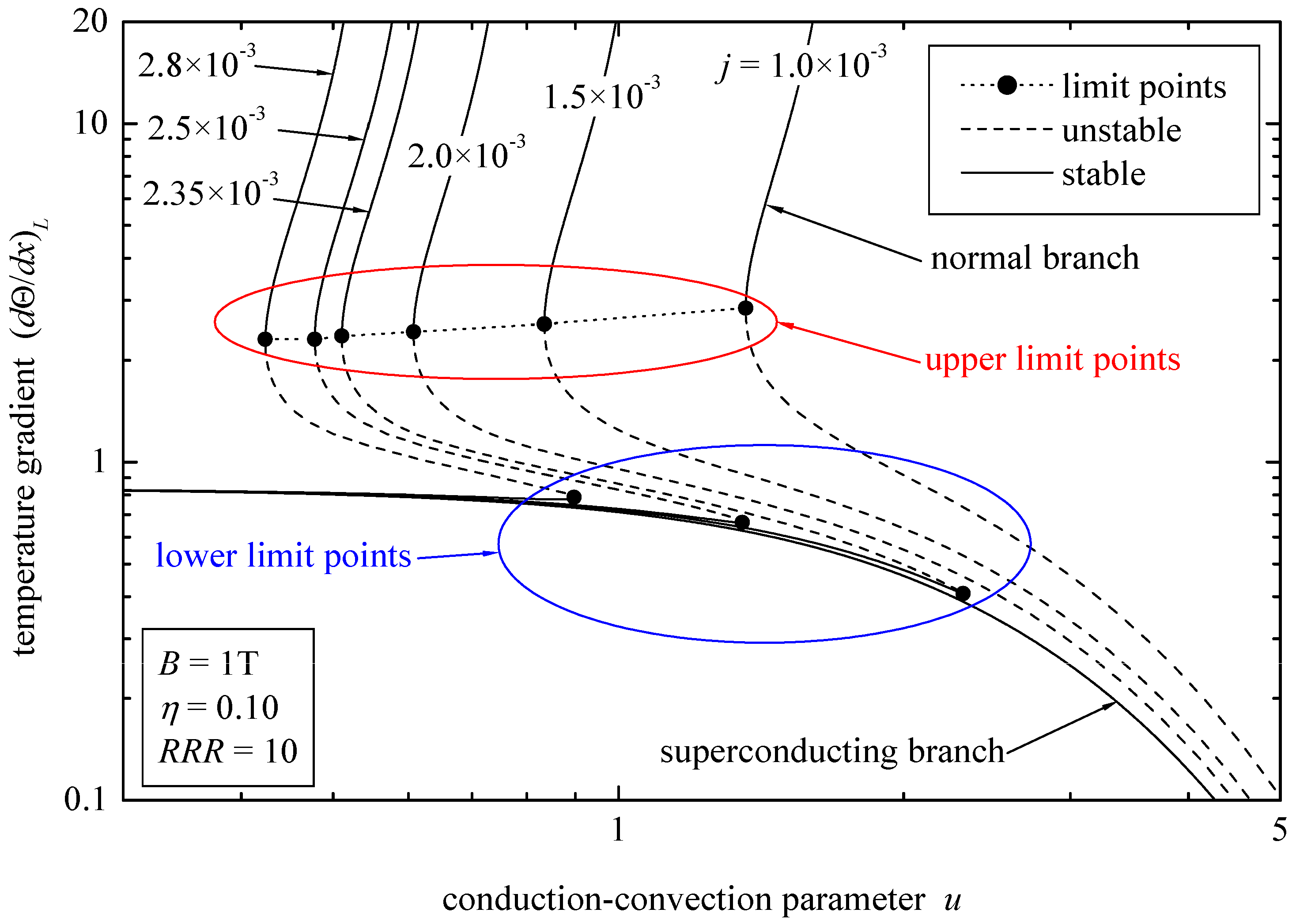
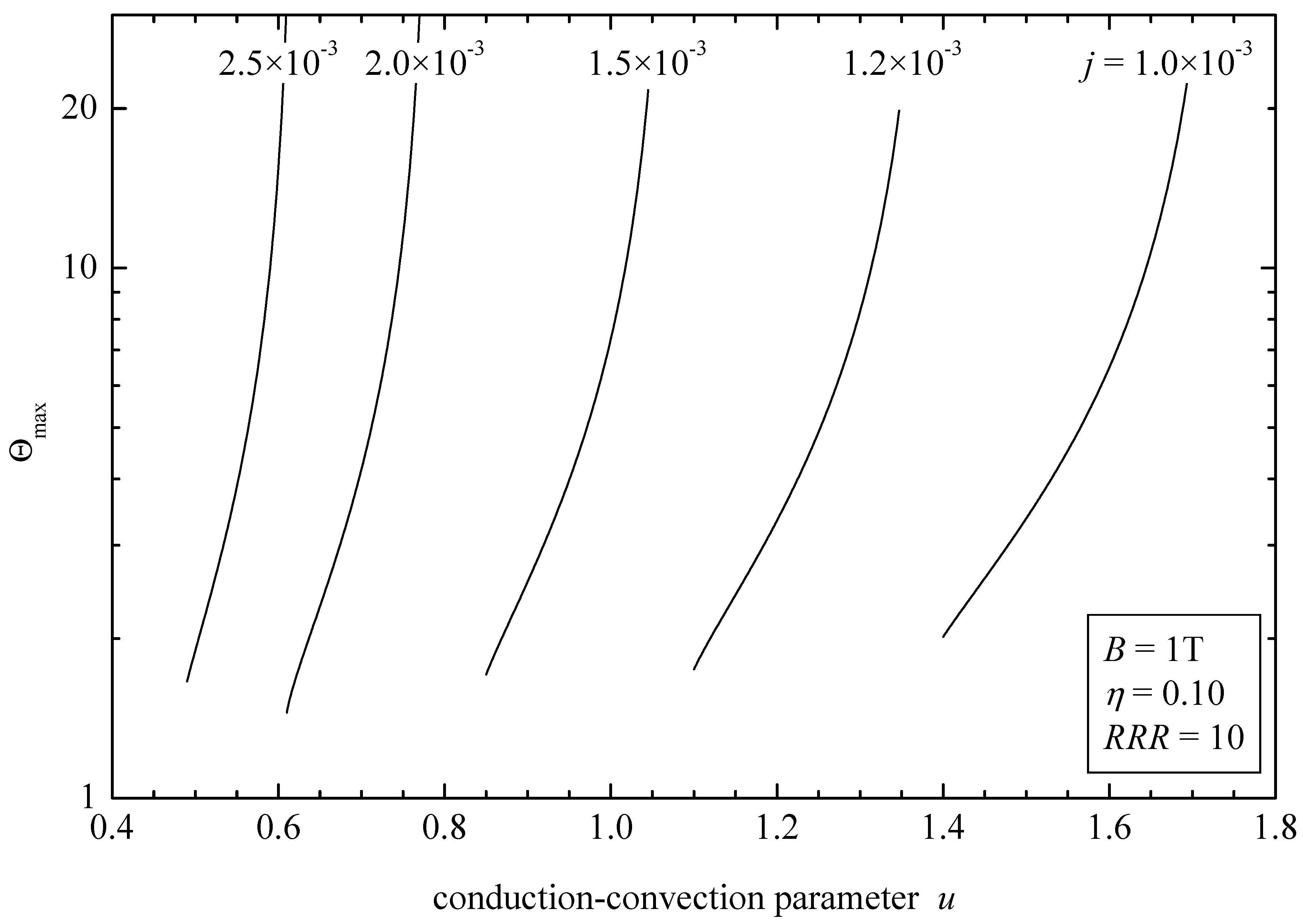
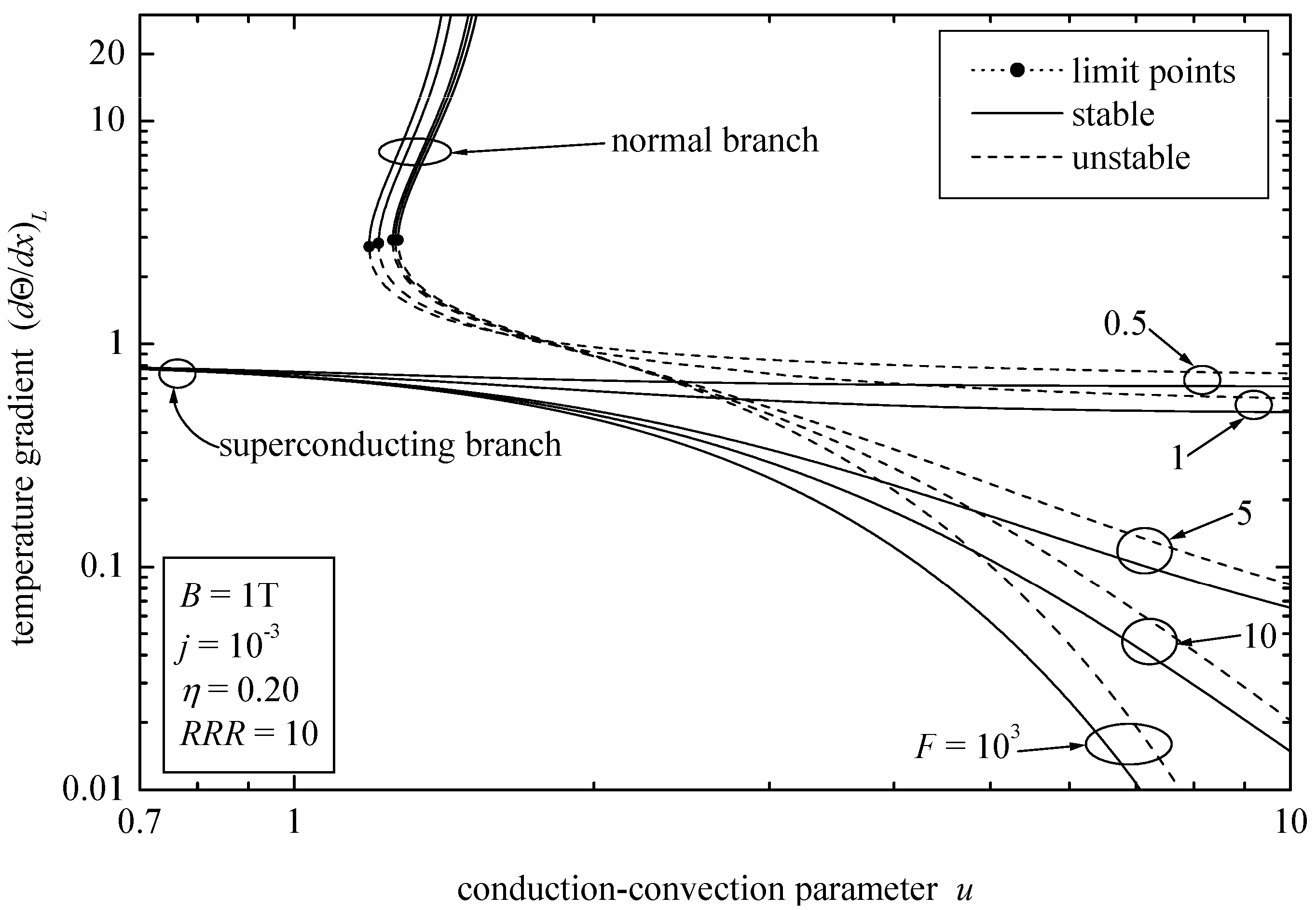
• For a specified current density and low filling ratios $\left(\eta \sim 0.1\right)$, no solution exists when u exceeds the lower limit point, i.e., $u>u_{\mathrm{LP}}^l$ (Figure 2).
• The upper limit point $u_{\mathrm{LP}}^u$ where the multiplicity region begins is a function of the applied current (Figure 2).
• Very high temperatures are predicted along the normal branch of steady states. The maximum temperature is a very sensitive function of the conduction–convection parameter and the applied current (Figure 7 and Figure 9).
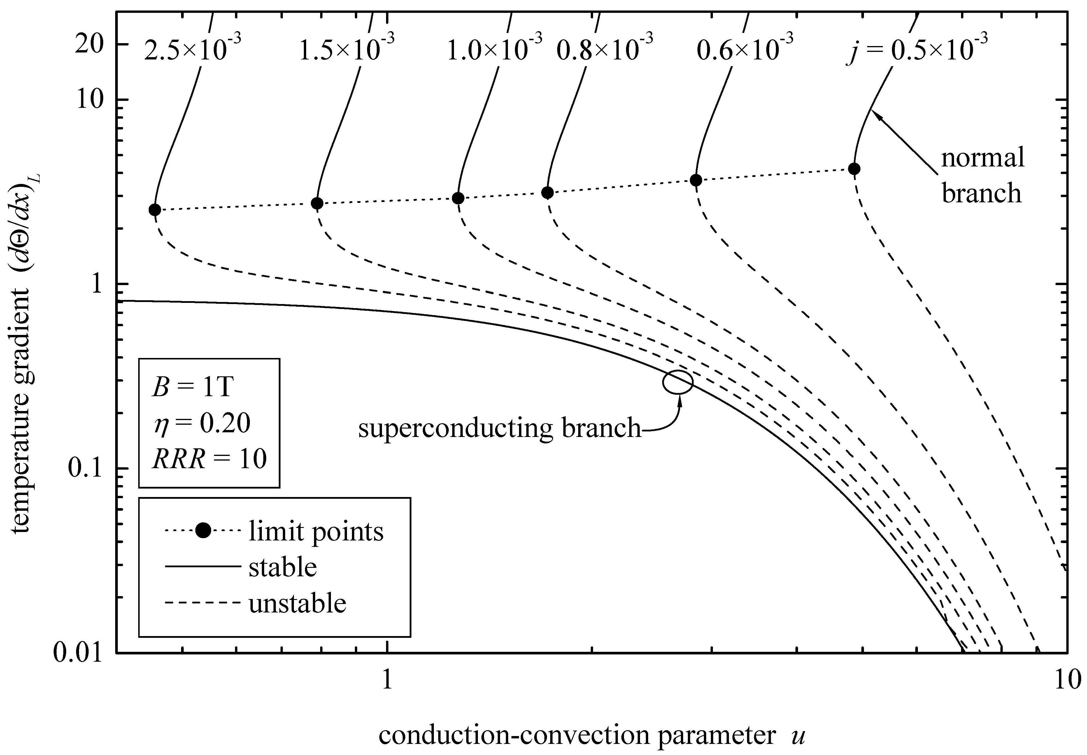
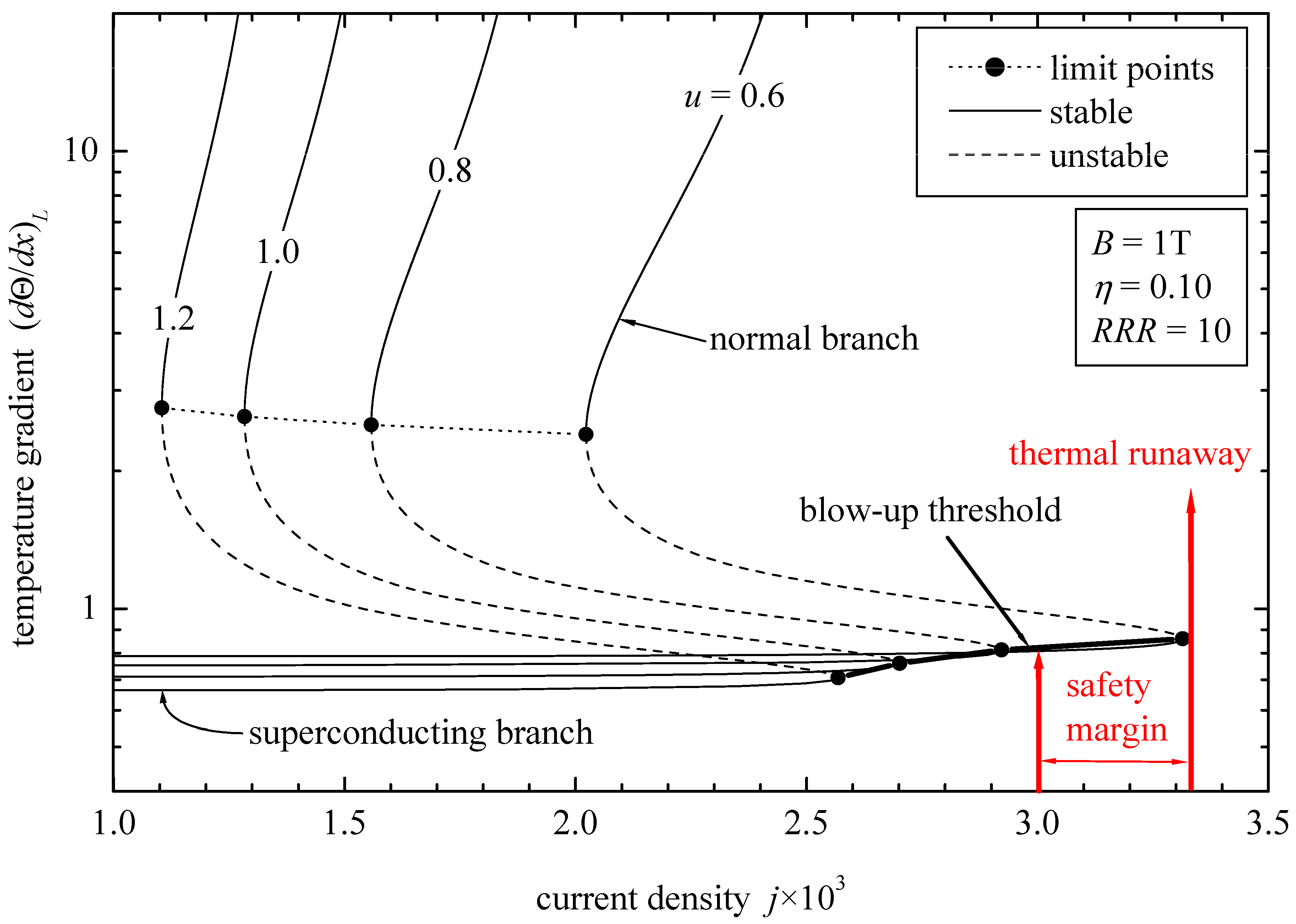
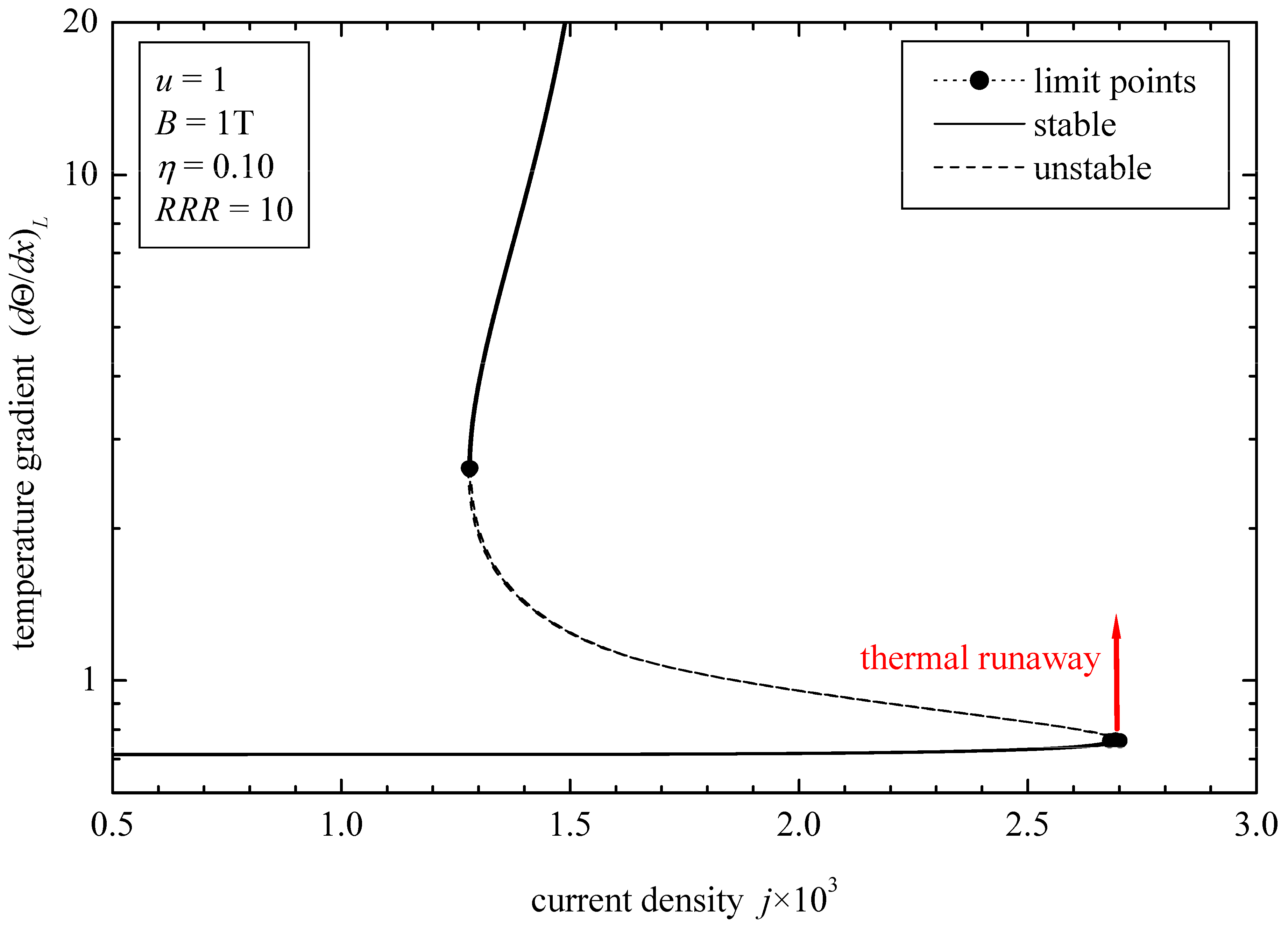
• Similar to the case of the metallic current leads, a temperature blow-up threshold exists defined by the lower limit points, which depend on the applied current and the conduction–convection parameter, beyond which thermal runaway is encountered (Figure 8).

The very existence of multiple solutions, and especially the lower limit points $u_{\mathrm{LP}}^l$ and $j_{\mathrm{LP}}^l$ associated with them, has a profound practical significance. From the design point of view, on one hand the higher the CCP, the lower the temperature gradient on the cold side. On the other hand, as the CCP increases, the safety margin towards $u_{\mathrm{LP}}^l$ decreases and the current lead is more susceptible to instabilities. This is similar to the case from the operating point of view, where the high value of the applied current will result in the reduction in the safety margin towards $j_{\mathrm{LP}}^l$. Therefore, a complete safety analysis of HTS current leads, apart from the temperature monitoring sensors connected with the protecting devices, should also take into account the design and operating margins towards $u_{\mathrm{LP}}^l$ and $j_{\mathrm{LP}}^l$, as demonstrated in the present study.

References

1. Bendorz, J.G.; Müller, K.A. Possible high-Tc superconductivity in the Ba-La-Cu-O system. Z. Physic Condens. Matter 1986, B64, 189–193. [Google Scholar]
2. Wesche, R.; Heller, R.; Bruzzone, P.; Fietz, W.H.; Lietzow, R.; Vostner, A. Design of high temperature superconductor current leads for ITER. Fusion Eng. Des. 2007, 82, 1385–1390. [Google Scholar] [CrossRef]
3. Ding, K.; Zhou, T.; Liu, C.; Du, Q.; Fernandez, A.V.; Zhu, S.; Devred, A.; Bauer, P.; Feng, H.; Fernandez-Hernando, L.; et al. Results of the testing of ITER CC HTS current leads prototypes. IEEE Trans. Appl. Supercond. 2016, 26, 4803404. [Google Scholar] [CrossRef]
4. Ballarino, A. Operation of 1074 HTS current leads at the LHC: Overview of three years of powering the accelerator. IEEE Trans. Appl. Supercond. 2013, 23, 4801904. [Google Scholar] [CrossRef]
5. Marshall, W.S.; Bai, H.; Bird, M.D.; Dixon, I.R.; Gavrilin, A.V.; Laureijs, G.A.; Lu, J.; Ouden, A.D.; Wijnen, F.J.P.; Wulffers, C.A.; et al. Fabrication and Testing of the 20 kA Binary Current Leads for the NHMFL Series-Connected Hybrid Magnet. IEEE Trans. Appl. Supercond. 2016, 26, 1–4. [Google Scholar] [CrossRef]
6. Raach, H.; Schroeder, C.H.; Floch, E.; Bleile, A.; Schnizer, P.; Andersen, T.P. 14 kA HTS Current Leads with one 4.8 K Helium Stream for the Prototype Test Facility at GSI. Phys. Procedia 2015, 67, 1098–1101. [Google Scholar] [CrossRef]
7. Drotziger, S.; Buscher, K.-P.; Fietz, W.H.; Heiduk, M.; Heller, R.; Hollik, M.; Lange, C.; Lietzow, R.; Moennich, T.; Richter, T.; et al. Overview of results from Wendelstein7-X HTS current lead testing. Fusion Eng. Des. 2013, 88, 1585–1588. [Google Scholar] [CrossRef]
8. Isono, T.; Hamada, K.; Okuno, K. Design optimization of a HTS current lead with large current capacity for fusion application. Cryogenics 2006, 46, 683–687. [Google Scholar] [CrossRef]
9. Kovalev, I.; Surin, M.; Naumov, A.; Novikov, M.; Novikov, S.; Ilin, A.; Polyakov, A.; Scherbakov, V.; Shutova, D. Test results of 12/18 kA ReBCO coated conductor current leads. Cryogenics 2017, 85, 71–77. [Google Scholar] [CrossRef]
10. Diev, D.N.; Galimov, A.R.; Ilin, A.A.; Khodzhibagiyan, H.G.; Kovalev, I.A.; Makarenko, M.N.; Naumov, A.V.; Novikov, M.S.; Novikov, S.I.; Polyakov, A.V.; et al. HTS current leads for the NICA accelerator project. Cryogenics 2018, 94, 45–55. [Google Scholar] [CrossRef]
11. Heller, R.; Fietz, W.H.; Kienzler, A. High power high temperature superconductor current leads at KIT. Fusion Eng. Des. 2017, 125, 294–298. [Google Scholar] [CrossRef]
12. Wilson, M.N. Superconducting Magnets; Oxford University Press: New York, NY, USA, 2002. [Google Scholar]
13. Iwasa, Y. Case Studies in Superconducting Magnets. Design and Operational Issues, 2nd ed.; Springer: New York, NY, USA, 2009. [Google Scholar]
14. Dresner, L. Stability of Superconductors; Springer+Bussiness Media: New York, NY, USA, 1995. [Google Scholar]
15. Romanovskii, V.R. Basic Macroscopic Principles of Applied Superconductivity; CRC Press: Boca Raton, FL, USA, 2021. [Google Scholar]
16. Paul, W.; Chen, M.; Lakner, M.; Rhyner, J.; Braun, D.; Lanz, W. Fault current limiter based on high temperature superconductors—Different concepts, test results, simulations, applications. Phys. C 2001, 354, 27–33. [Google Scholar] [CrossRef]
17. Lee, H.G.; Kim, H.M.; Lee, B.W.; Oh, I.S.; Hyun, O.B.; Sim, J.; Chang, H.M.; Bascunan, J.; Iwasa, Y. Conduction-Cooled Brass Current Leads for a Resistive Superconducting Fault Current Limiter (SFCL) System. IEEE Trans. Appl. Supercond. 2007, 17, 2248–2251. [Google Scholar] [CrossRef]
18. Noe, M.; Hobl, A.; Tixador, P.; Martini, L.; Dutoit, B. Conceptual Design of a 24 kV, 1 kA Resistive Superconducting Fault Current Limiter. IEEE Trans. Appl. Supercond. 2011, 22, 5600304. [Google Scholar] [CrossRef]
19. Sarkar, D.; Roy, D.; Choudhury, A.; Yamada, S. Performance analysis of saturated iron core superconducting fault current limiter using Jiles–Atherton hysteresis model. J. Magn. Magn. Mater. 2015, 390, 100–106. [Google Scholar] [CrossRef]
20. Farokhiyan, M.; Hosseini, M.; Kavousi-Fard, A. Current density distribution in resistive fault current limiters and its effect on device stability. Phys. C 2020, 580, 1353786. [Google Scholar] [CrossRef]
21. Zhang, J.; Dai, S.; Ma, T.; Li, Y.; He, D. Current limiting characteristics of a resistance-inductance type superconducting fault current limiter. Phys. C 2022, 601, 1354105. [Google Scholar] [CrossRef]
22. Sotelo, G.G.; dos Santos, G.; Sass, F.; França, B.W.; Dias, D.H.N.; Fortes, M.Z.; Polasek, A.; de Andrade, R., Jr. A review of superconducting fault current limiters compared with other proven technologies. Superconductivity 2022, 3, 100018. [Google Scholar] [CrossRef]
23. Jones, M.; Yeroshenko, V.; Starostin, A.; Yaskin, L. Transient behaviour of helium-cooled current leads for superconducting power transmission. Cryogenics 1978, 18, 337–343. [Google Scholar] [CrossRef]
24. Aharonian, G.; Hyman, L.; Roberts, L. Behaviour of power leads for superconducting magnets. Cryogenics 1981, 21, 145–151. [Google Scholar] [CrossRef]
25. Buchs, K.; Hyman, L.G. Investigation of multiple solutions for gas cooled current leads and results of survey information on current leads. Cryogenics 1983, 23, 362–366. [Google Scholar] [CrossRef]
26. Krikkis, R.N. Multiplicities and thermal runaway of current leads for superconducting magnets. Cryogenics 2017, 83, 8–16. [Google Scholar] [CrossRef]
27. Mumford, F.J. Superconducting current-leads made from high Tc superconductor and normal metal conductor. Cryogenics 1989, 29, 206–207. [Google Scholar] [CrossRef]
28. Hull, J.R. High temperature superconducting leads for cryogenic apparatus. Cryogenics 1989, 29, 1116–1123. [Google Scholar] [CrossRef]
29. Dresner, L. Superconductor stability 90: A review. Cryogenics 1991, 31, 489–498. [Google Scholar] [CrossRef]
30. Wesche, R.; Fuchs, A. Design of superconducting current leads. Cryogenics 1994, 34, 145–154. [Google Scholar] [CrossRef]
31. Lee, H.; Kim, H.M.; Iwasa, Y.; Kim, K.; Arakawa, P.; Laughon, G. Development of vapor-cooled HTS-copper 6-kA current lead incorporating operation in the current-sharing mode. Cryogenics 2004, 44, 7–14. [Google Scholar] [CrossRef]
32. Jang, J.Y.; Lee, W.S.; Kang, J.S.; Jo, H.C.; Hwang, Y.J.; Na, J.B.; Sim, K.; Kim, H.M.; Yoon, Y.S.; Do Chung, Y.; et al. Experimental study of the new type of hts elements for current leads to be applied to the nuclear fusion devices. IEEE Trans. Appl. Supercond. 2012, 22, 4801204. [Google Scholar] [CrossRef]
33. Drotziger, S.; Fietz, W.H.; Heiduk, M.; Heller, R.; Lange, C.; Lietzow, R.; Mohring, T. Investigation of HTS Current Leads Under Pulsed Operation for JT-60SA. IEEE Trans. Appl. Supercond. 2011, 22, 4801704. [Google Scholar] [CrossRef]
34. Heller, R.; Bauer, P.; Savoldi, L.; Zanino, R.; Zappatore, A. Predictive 1-D thermal-hydraulic analysis of the prototype HTS current leads for the ITER correction coils. Cryogenics 2016, 80, 325–332. [Google Scholar] [CrossRef]
35. Han, Q.; Ding, K.; Lu, K.; Liu, C.; Liu, C.; Huang, X.; Zhou, T.; Song, Y. Safety analysis of the 100 kA current lead for CFETR. Fusion Eng. Des. 2020, 153, 111481. [Google Scholar] [CrossRef]
36. Dong, Y.; Ran, Q.; Lu, K.; Zheng, J.; Liu, C.; Liu, H.; Ding, K. Structure, design and test of 13 kA HTS current lead. Cryogenics 2023, 132, 103620. [Google Scholar] [CrossRef]
37. Chang, H.-M.; Kim, N.H.; Oh, S. Thermodynamic optimization of 10–30 kA gas-cooled current leads with REBCO tapes for superconducting magnets at 20 K. Cryogenics 2023, 131, 1036667. [Google Scholar] [CrossRef]
38. Bottura, L. Critical Surface for BSCCO-2212 Superconductor; Note CRYO/02/027; CryoSoft Library CERN: Thoiry, France, 2002. [Google Scholar]
39. van der Laan, D.C.; van Eck, H.J.N.; Haken, B.T.; Schwartz, J.; ten Kate, H.H.J. Temperature and Magnetic Field Dependence of the Critical Current of BSCCO Tape Conductors. IEEE Trans. Appl. Supercond. 2001, 11, 3345–3348. [Google Scholar] [CrossRef]
40. Wesche, R. Temperature dependence of critical currents in superconducting Bi-2212/Ag wires. Phys. C 1995, 246, 186–194. [Google Scholar] [CrossRef]
41. Romanovskii, V.; Watanabe, K. Multi-stable static states of Bi-based superconducting composites and current instabilities at various operating temperatures. Phys. C 2005, 420, 99–110. [Google Scholar] [CrossRef]
42. Dresner, L. Stability and protection of Ag/BSCCO magnets operated in the 20–40 K range. Cryogenics 1993, 33, 900–909. [Google Scholar] [CrossRef]
43. Lim, H.; Iwasa, Y. Two-dimensional normal zone propagation in BSCCO-2223 pancake coils. Cryogenics 1997, 37, 789–799. [Google Scholar] [CrossRef]
44. Krikkis, R.N.; Sotirchos, S.V.; Razelos, P. Analysis of multiplicity phenomena in longitudinal fins under multi-boiling conditions. ASME J. Heat Transf. 2004, 126, 1–7. [Google Scholar] [CrossRef]
45. Krikkis, R.N. On the multiple solutions of boiling fins with heat generation. Int. J. Heat Mass Transf. 2015, 80, 236–242. [Google Scholar] [CrossRef]
46. Krikkis, R.N. Laminar conjugate forced convection over a flat plate. Multiplicities and stability. Int. J. Therm. Sci. 2017, 111, 204–214. [Google Scholar] [CrossRef]
47. Krikkis, R.N. On the Thermal Dynamics of Metallic and Superconducting Wires. Bifurcations, Quench, the Destruction of Bistability and Temperature Blowup. J 2021, 4, 803–823. [Google Scholar] [CrossRef]
48. Pfotenhauer, J.; Lawrence, J. Characterizing thermal runaway in HTS current leads. IEEE Trans. Appl. Supercond. 1999, 9, 424–427. [Google Scholar] [CrossRef]
49. Vysotsky, V.; Sytnikov, V.; Rakhmanov, A.; Ilyin, Y. Analysis of stability and quench in HTS devices—New approaches. Fusion Eng. Des. 2006, 81, 2417–2424. [Google Scholar] [CrossRef]
50. Romanovskii, V.R.; Watanabe, K. Operating modes of high Tc composite superconductors and thermal runaway conditions under current charging. Supercond. Sci. Technol. 2006, 19, 541–550. [Google Scholar] [CrossRef]
51. Werweij, A.P. Thermal Runaway of the 13kA busbar joints in the LHC. IEEE Trans. Appl. Supercond. 2010, 20, 2155–2159. [Google Scholar] [CrossRef]
52. Willering, G.P.; Bottura, L.; Fessia, P.; Scheuerlein, C.; Verweij, A.P. Thermal Runaways in LHC Interconnections: Experiments. IEEE Trans. Appl. Supercond. 2011, 21, 1781–1785. [Google Scholar] [CrossRef]
53. Maeda, H.; Yanagisawa, Y. Recent developments in high temperature superconducting magnet technology (review). IEEE Trans. Appl. Supercond. 2014, 24, 4602412. [Google Scholar] [CrossRef]
Figure 1. Geometry and energy balance on the current leads.
J 06 00022 g001
Figure 2. Bifurcation diagrams in the u , Θ L plane for η = 0.1 and F 1 .
J 06 00022 g002
Figure 3. Geometrical representation of the multiple-solution structure.
J 06 00022 g003
Figure 4. Bifurcation diagrams in the u , Θ L plane for η = 0.2 and F 1 .
J 06 00022 g004
Figure 5. Temperature profiles for u = 0.8 and 0.9, F 1 .
J 06 00022 g005
Figure 6. Temperature profiles for u = 2 and 3, F 1 .
J 06 00022 g006
Figure 7. Effect of u on maximum temperature along the normal branch, F 1 .
J 06 00022 g007
Figure 8. Bifurcation diagrams in the j , Θ L plane for η = 0.1 and F 1 .
J 06 00022 g008
Figure 9. Effect of j on maximum temperature along the normal branch, F 1 .
J 06 00022 g009
Figure 10. Effect of F on the bifurcation diagrams on the u , Θ L plane.
J 06 00022 g010
Figure 11. Effect of F on the bifurcation diagrams on the j , Θ L plane. F = 10 3 , 10, 5 and 1.
J 06 00022 g011