Review

Offshore Electrical Grid Layout Optimization for Floating Wind—A Review

by
Magnus Daniel Kallinger
1,2,*,
José Ignacio Rapha
1,
Pau Trubat Casal
2 and
José Luis Domínguez-García
1
1
Power Systems Group, Catalonia Institute for Energy Research (IREC), Jardins de les Dones de Negre 1, 2a, Sant Adrià de Besòs, 08930 Barcelona, Spain
2
Department of Civil and Environmental Engineering, Universitat Politècnica de Catalunya (UPC), Jordi Girona 1-3, 08034 Barcelona, Spain
*
Author to whom correspondence should be addressed.
Clean Technol. 2023, 5(3), 791-827; https://doi.org/10.3390/cleantechnol5030039
Submission received: 24 April 2023 / Revised: 8 June 2023 / Accepted: 21 June 2023 / Published: 26 June 2023
(This article belongs to the Collection Review Papers in Clean Technologies)

Abstract

:
Electrical grid layout optimization should consider the placements of turbines and substations and include effects such as wake losses, power losses in cables, availability of different cable types, reliability-based power losses and operational/decommissioning cost besides the initial investment cost. Hence, optimizing the levelized cost of energy is beneficial capturing long-term effects. The main contribution of this review paper is to identify the current works and trends on electrical layout optimization for offshore wind farms as well as to analyze the applicability of the found optimization approaches to commercial-scale floating wind farms which have hardly been investigated so far. Considering multiple subproblems (i.e., micrositing and cabling), simultaneous or nested approaches are advantageous as they avoid sequential optimization of the individual problems. To cope with this combinatorial problem, metaheuristics seems to offer optimal or at least close-to-optimal results while being computationally much less expensive than deterministic methods. It is found that floating wind brings new challenges which have not (or only insufficiently) been considered in present optimization works. This will also be reflected in a higher complexity and thus influence the suitability of applicable optimization techniques. New aspects include the mobility of structures, the configurations and interactions of dynamic cables and station-keeping systems, the increased likelihood of prevailing heterogeneous seabeds introducing priority zones regarding anchor and riser installation, the increased importance of reliability and maintainability due to stricter weather limits, and new floating specific wind farm control methods to reduce power losses. All these facets are crucial to consider when thoroughly optimizing the levelized cost of energy of commercial-scale floating offshore wind farms.

1. Introduction

Bottom-fixed offshore wind structures are limited to a certain water depth. It is often referred to as a threshold of 60m, after which this type of substructure can no longer be installed economically. Keeping in mind that around 80% of the world’s potential offshore wind capacity is located in waters deeper than that [1], floating wind rose to the occasion as a new, disruptive technology. All over the world, countries are looking for feasible options to generate green energy. For countries/regions that do not have any or very limited experience in offshore wind due to complex bathymetry and/or problematic soil conditions, floating wind makes it possible to install projects in previously inaccessible regions in order to harvest offshore energy. The sites, now possibly being located farther offshore, typically offer stronger and steadier wind conditions that make it possible to increase the captured power and therefore lower the levelized cost of energy (LCOE). However, the relatively nascent technology is yet more expensive and less reliable than bottom-fixed offshore installations due to the geographical conditions of the open ocean but also due to its relatively low technology readiness level. The high cost is due to the construction of the large turbine foundations, using deep water mooring systems to ensure the turbines endure the prevailing dynamic conditions and the necessity of using dynamic subsea cables in order to collect the energy from the floating system. The low reliability is mainly due to the poor accessibility of the floating offshore wind farms (FOWFs). Weather conditions farther offshore are likely to be worse, whereas weather limits for repair works are stricter due to the floating behavior. The possibly large distances from shore result in longer travel times, which create the need for suitable weather windows. If a fault occurs in any of the facilities, the effects last longer, leading to a deterioration in reliability. Therefore, FOWFs must be planned carefully from both an economical and reliability perspective.
Offshore wind farms (OWF) are typically designed in a sequential planning process. As a first step, a suitable area at sea is identified which can be used for power production. Second, the area is populated with wind turbines (WTs) in the micrositing process which typically tries to exploit the maximum annual energy production (AEP) considering wake effects on downstream turbines within the designed wind farm. If applicable, the micrositing process usually also deals with the positioning of an offshore substation (OSS) in the wind farm area. In a last step, the fixed WT (and OSS) positions are used to carry out the cable routing optimization [2]. This process offers a robust and computationally less cumbersome solution but does not take the full complexity of the combinatorial problem into consideration. The conservative micrositing process will try to maximize the distance between individual WTs in order to reduce wake effects, which will have a large impact on future offshore wind farms consisting of larger and more powerful turbines. The increased distance between WTs will result in longer inter-array cables forcing an increase in capital expenditures (CAPEX) and power losses over the OWF’s lifetime. Even though power losses can be mitigated by taking advantage of different cable sizes, the selection of the optimal cable diameter for a WT interconnection increases the complexity of the overall optimization. The problem becomes even more convoluted when considering the increasing size of future OWFs, as well as their increasing distance to shore, since both factors strongly favor the use of at least one or even multiple offshore substations (OSS) where the power is collected and transformed into a high-voltage export system which, depending on the distance to shore, can be either an AC or DC system. Optimally placing and interconnecting the OSS(s) brings a new dimension to the optimization as it will have a major effect on the inter-array collection system as well as on the HV export system.
According to Serrano González et al. [3], the cost for the electrical infrastructure of a bottom-fixed offshore wind farm accounts for 15–30% of the total acquisition cost (CAPEX). Hence, optimizing the cabling and possibly the overall OWF layout offers a great opportunity for cost saving. However, most of the literature on cabling layout optimization is primarily developed for the bottom-fixed offshore wind industry, and the future trend towards floating wind farms has not yet been thoroughly assessed. It can be assumed that this cost share for the electrical infrastructure will be similar for commercial-sized FOWFs. However, due to the increased complexity, the yet-missing experience in FOWF deployment, and the lack of component standardization ([4]), it is assumed that the absolute cost will be much higher. As a consequence of the high cost, the complexity of the overall planning procedure and the low accessibility for repair work (especially for floating wind), the cable layout optimization for floating wind applications is estimated to be a very valuable area for future research activities.
This review paper aims to analyze cable layout optimization techniques primarily developed for the bottom-fixed offshore wind industry and assesses their applicability to future commercial-sized FOWFs. The outcome highlights areas and engineering constraints which will require thorough consideration in order to design reliable FOWFs with long-term economic benefits.
The remainder of this paper is organized as follows: In Section 2, the literature focusing on bottom-fixed industry is examined in terms of applied optimization techniques and considered engineering constraints. Section 3 points out optimization techniques with a focus on FOWFs, followed by the discussion Section 4 in which floating wind specific aspects and constraints are identified which need to find consideration in future broader optimization works. Finally, the findings are summarized in Section 5.

2. Bottom-Fixed Literature Approaches

The broad majority of the literature handling the inter-array cabling optimization is focused on the traditional bottom-fixed offshore wind industry. Only a very limited number of publications can be found which handle the matter with regard to floating wind and tackle some of the new challenges that arise with the new technology, as can be seen in the comparison of the studied literature in Figure 1.
Hence, in this section, an overview is presented on how the optimization problem is addressed in the bottom-fixed case. Special attention was given to works published since 2019 since extensive review papers ([5,6], both from 2019) deal with earlier works.
In general, it can be said that due to the complexity of the overall optimization framework, different approaches developed in the literature concentrate on certain parts of the problem while neglecting others.
In the further course of this section, the investigated literature is examined.

2.1. Objectives and Common Constraints

Before going deeper into the optimization practices, it is important to clarify what is to be optimized in the first place. The most obvious and also the easiest to implement is to minimize the total cable length, because this is usually what everything depends on in the first place: the acquisition cost, the losses in the cables, the trenching length (in case of buried cables), etc. However, this optimization starts to fail as soon as several cable types with different capacities are considered, which are typically subject to different cost factors and represent different electrical impedances.
Furthermore, the question arises whether only a snapshot or a time period (e.g., the lifetime of the wind farm) should be optimized. Thus, not only the CAPEX but also the OPEX or even possibly DECEX must be included. In case of OPEX, in addition to the electrical losses, there may also be failure rates which possibly trigger unavailabilities due to long-lasting repair works, which have a negative impact on the annual energy produced (AEP) and therefore on the turnover. The most complete optimization objective can therefore be the LCOE taking into account the entire lifetime performance of the OWF.
Although different approaches are used in the literature (e.g., the optimization objective or the techniques), there are some commonalities that make a meaningful simulation possible. A common approach in the literature is to exclude the crossing or even the shared trajectory of cables. It must be noted that cable crossings are not impossible in principle but, especially for buried cable sections, this is a sensible constraint. Trenching and cable-laying in the close vicinity of already-laid cables increases the risk of mechanical damage on both cables. However, not just the installation could influence the cable’s performance but also the operation itself. For example, heat generated by the Ohmic resistance can damage the cables, and partial discharges in one cable could therefore influence the performance of the other cable implying that two crossing cables would have to be insulated against each other. Furthermore, O&M activities would be more time-consuming. In case the cable that is buried lowest fails and has to be replaced, both cables would have to be dug up, resulting in considerably higher costs.
For optimizing the inter-array cabling, most works only consider the Euclidean distance between WTs. This is a valid approach considering that those works only take a flat homogeneous seabed into account. However, this simplification is broadly assumed but does not reflect real conditions especially as OWFs become ever-larger, requiring more and more space, enlarging the footprint on the seabed and making it therefore more likely that a non-homogeneous seafloor and even possible restriction zones will be encountered on-site. Works that raise this issue will be highlighted in the further course of this review and the taken approaches to overcome this problem will be explained.

2.2. Topologies

It is a very common approach in the literature to restrict the cable layout to a topology prior to the optimization. However, the interconnection of offshore wind turbines is governed by the preferred topology since it heavily influences the length of the cabling, the electrical losses, the OWF reliability, and so on. It should therefore be generally avoided to exclude one topology from the beginning [7]. However, there are two main topologies which are widely discussed in the literature. Each topology developed in the literature comes with its own adaptations so that a variety of possible layouts exist.

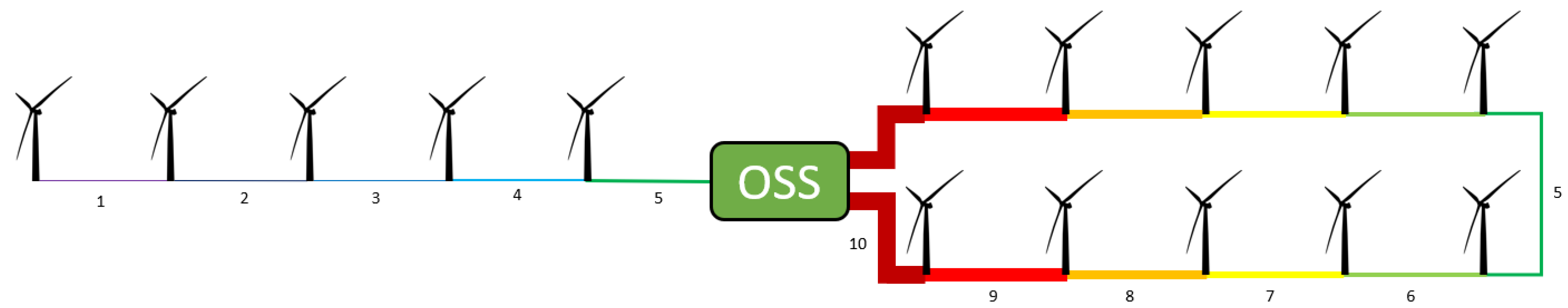
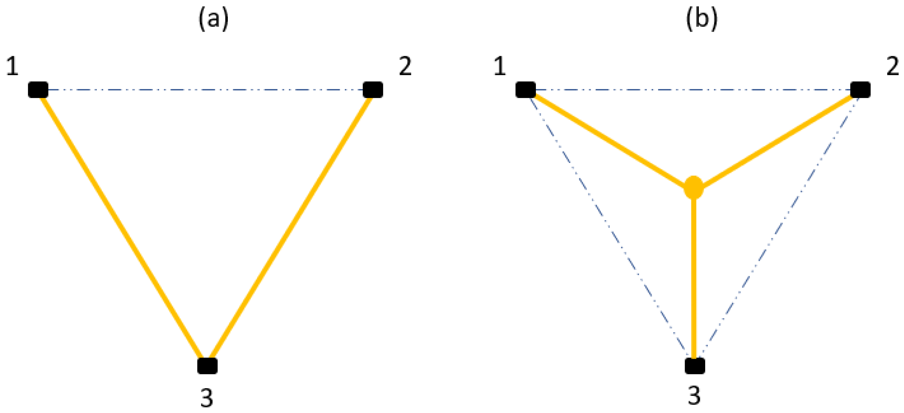
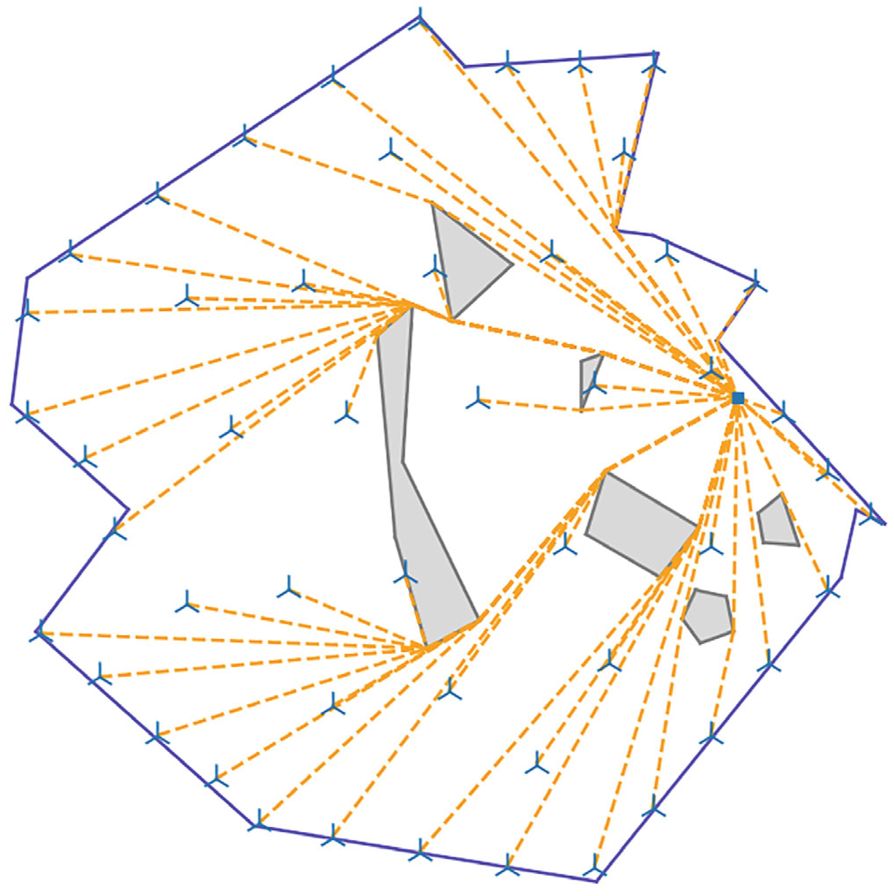
2.2.1. Branched Topology

The branched topology connects WTs in a branch to the offshore substation. In a branch, multiple cables are allowed to connect to a WT but only one cable is allowed to transmit the power away from the WT towards the subsequent receiver (either another WT or an OSS). Based on the N-1 requirement, the cable selection per WT interconnection only needs to support all its downstream turbines, which leaves room for further optimization. Hence, this problem can be modeled using a Capacitated Minimum Spanning Tree (C-MST) considering that the largest available cable needs to be able to support the power capacity [5]. The branched topology is sometimes prevented at the beginning of the optimization by introducing restrictions. This is due to the fact that this type of cabling is associated with a higher investment and installation effort regarding additional electrical components (e.g., switchgears, (dis-)connectors and/or offshore transformer modules (OTMs are able to handle the transformer function directly at the WT and allow it to be directly connected to shore [8])), for which it may already be clear in advance that they may not be available [5].
Hence, an adaptation of the branched layout exists—a subset of this topology named the radial topology. It connects turbines in a string with at most only one cable entering and one cabling exiting each turbine. It is important to note that as a subset of the branched topology, the radial connection cannot deliver shorter cable paths but can ease the computational effort since it considers engineering constraints from the beginning [9]. In commercial-scale OWFs, the radial connection scheme is widely used at present since it is a relatively simple layout and offers a high degree of flexibility in control while simultaneously coming with low initial investment cost.
However, both, the branched as well as the radial topology lack redundancy, as a failure in an upstream centric branch will force all downstream WTs to shut down since the power can not be transferred to a receiver [10]. Nevertheless, the broad use of this topology is often justified by the fact that buried submarine cables show relatively low failure rates (between 0.08% and 1.5% per km and year [11]) compared to other components. However, besides the stated lower failure rates, Young [12] states that cable failures account for up to 77% of the total global cost of OWF losses and that 95% of all offshore wind projects experience one or more cable-related insurance claims. These may be due to incorrect cable installation or operation while the latter translates to electrical faults in around 20% of failures. Especially for large-scale wind farms which are located farther from shore, the consequence of a cable failure could be dramatic, as a failure could last for two to three months due to sea cables’ low accessibility and long mean times to repair (MTTR) causing large losses of revenue connected with expected but not supplied energy (EENS) depending on the failure location [13].

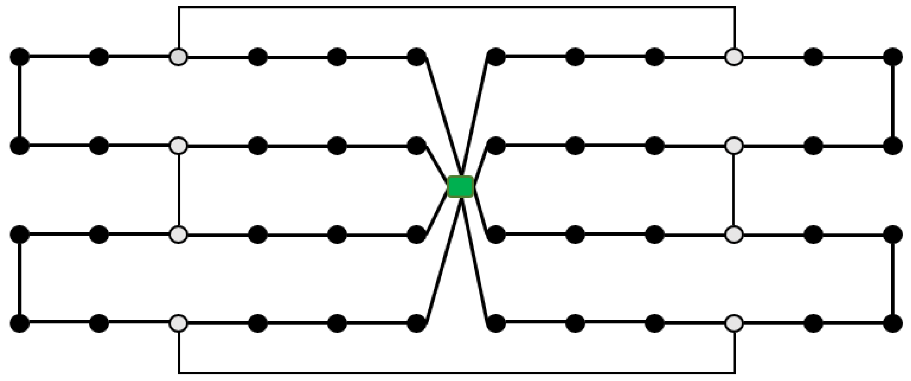
2.2.2. Ring Structure

To enhance the redundancy and therefore the reliability of the offshore collector network, the loop or ring structure is proposed in the literature as it allows a bi-directional power transmission to the OSS [14]. However, the looped structure comes with higher installation cost due to the longer cabling route, the need to deploy larger cables with higher ratings and electrical components such as reconfiguration switches. Furthermore, it requires a higher level of control. Typically, cable ratings in a ring structure are selected to be equal ([13]) but like in the branched case, connections only need to be able to support all the downstream turbines as can be seen in Figure 2.
The looped structure corresponds to a Capacitated Vehicle Routing Problem (CVRP) with the OSS, the WTs, and cable capacities being the depot, customers, and vehicle capacities, respectively.
Despite the higher investment cost, it is argued that the ring design would save enough money during the operation of the OWF that it would be the most economical solution in long-term assessments [15].

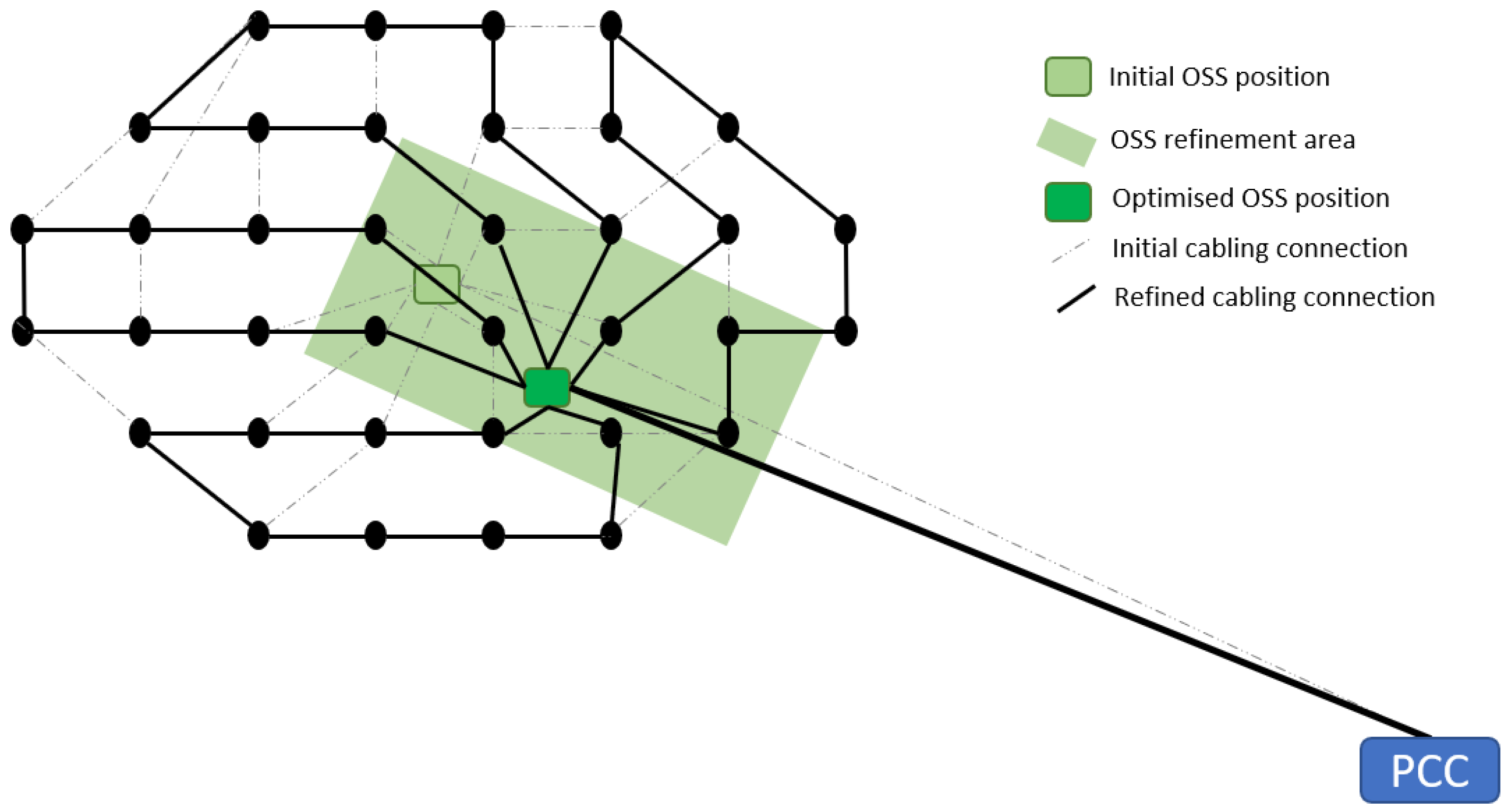
2.3. Clustering and OSS Positioning

Large and distant OWFs require the application of one or even more OSS(s) in order to transmit the generated power without larger power losses to the point of common coupling (PCC) with the onshore grid. Hence, most papers consider flexible or pre-determined locations of the OSSs in their work as they form the root of the inter-array cabling structure and will therefore have a large impact on the objective or fitness function. Pérez-Rúa and Cutululis [5] identified three approaches which are commonly found in the literature in order to position the OSS(s) in the OWF area and to allocate multiple WTs to them:
Approach (1) is the simultaneous approach, in which the allocation of WTs is solved concurrently with the cabling problem. For large OWFs, this high-quality approach typically comes with major computational expenses, especially when using deterministic methods which are explained in more detail in Section 2.4.1.
Approach (2) consists of multiple steps starting with the creation of clusters within the OWF, locating a central OSS in each cluster, and then solving the inter-array cabling problem in a subsequent step. The clustering may be carried out (but rarely applied in the literature) mathematically or via clustering algorithms. Clustering algorithms split the OWF into smaller subgroups by maximizing similarities of individual WTs in a subgroup (such as minimizing the mean distance of WTs to an OSS location) while minimizing similarities of individuals belonging to different groups. By creating subgroups of previously obtained or pre-determined OWF layouts, the inter-array cabling can be simplified in order to find a good initial or at least feasible initial solution for the interconnection faster. This holds especially true once the number of WTs becomes larger which would result in a larger computational burden. However, the main disadvantage of applying clustering as a pre-processing step is that the number of clusters typically needs to be pre-determined and that the subsequent cabling optimization is usually limited to being cluster-internal, so no overall optimization is carried out. Both effects narrow the solution search space for the overall problem optimization [16].
As representative clustering algorithms, there are quality threshold (QT) and K-means ([17,18,19,20]), as well as fuzzy C-means (FCM), algorithms ([13,14,21,22,23,24]).
The QT clustering method determines a cluster quality, e.g., the cluster diameter and the minimum number of WTs contained in each cluster ([25]), and performs clustering of WTs so that a certain threshold value for the diameter is not exceeded.
While QT methods use only the diameter as a clustering criterion, two criteria were introduced for K-clustering methods in [26]. One is the distance between WTs and the center of each group, while the other is the angle of each WT with respect to the OSS. Shin and Kim [17] point out that using the distance criteria, WTs in proximity can be connected to each other. However, when collecting the electricity far from the OSS, the main cables used between each feeder and the OSS may become longer which implies increased cost since cables with higher capacities are more expensive. The angle criterion naturally avoids crossings of collector cables to the OSS with any other cables within other clusters. Nevertheless, a local minimum can also not be easily avoided depending on the chosen number of clusters k and the initial angle of the WT allocation. Yi et al. [20] point out that the conventional K-clustering method is not able to find clusters with the same number of WTs, which will prevent equal capacity requirements in the case of multiple OSSs. This will have an impact on the economic efficiency. Therefore, they adapted the K-clustering solution by swapping memberships of WTs between any clusters until all clusters incorporate the same number of WTs and the sum of distances between WTs and OSS in each cluster is minimized. Furthermore, they notice that the OSS position in the cluster’s center is possibly too close to a WT. Hence, they manually realign the OSS position to comply with any given safety distance.
Fuzzy C-means clustering has been widely used in the literature and is therefore considered validated as a reliable clustering method. The FCM algorithm is an extension of the K-means clustering method with the feature that an object (WT) is allowed to be assigned to more than one cluster (OSS). This fuzzy overlap is made possible by the fact that a membership degree is introduced which is based on stochastic initialization which may result in unstable outputs.
Approach (3), commonly found in the literature in order to position the OSS(s) in the OWF area and to allocate multiple WTs, is the nested approach. It consists of a recurring calculation process, where the OSS position(s) and WT allocations are assessed in an outer loop while the specific cabling problem is addressed in an inner-loop. Zuo et al. [22] studied the connection of an older already-existing OWF with a newly built OWF consisting of more powerful turbines. Due to the large difference in turbine capacities over the geographic area, they used a weighted FCM clustering method which was further refined by the implementation of a pattern search algorithm (firstly implemented by Shin and Kim in [17]) in which the area around the FCM solution is proposed as a search space and undergoes further refinement per loop iteration. Pattern search is a heuristic-based optimization method which follows a predefined exploration pattern. As it can not guarantee a global optimum, modifications of the pattern are necessary in order to avoid falling into a local optimum. The modifications to the search space are dependent on whether a better OSS location could be found in the previous iteration loop or not [17].
In Figure 3, the chosen approaches for OSS positioning of analyzed studies published since 2019 are shown.
It is shown that the sequential approach (2) is the most commonly used in the newer offshore wind cabling optimization literature. This is partially due to the fact that some papers (mainly the ones following a deterministic approach) only take one predetermined OSS location into account in order to solve the complex cabling problem optimally in a reasonable amount of time. Furthermore, several yet-unestablished metaheuristics (i.e., compared to genetic algorithms (GA) and particle swarm optimizations (PSO)) concentrate on solving the cabling problem while considering a pre-assessed, fixed OSS location. Deterministic approaches which consider more than one possible but predetermined location for the OSS position are counted for as a simultaneous approach. However, it should be noted that no analyzed deterministic method accounts for free OSS positioning. The simultaneous approach using GAs and PSOs is often realized by passing genetic/particle information about the OSS location to the next generation of individuals/particles. This will be explained in more detail in Section 2.4.
Overall, clustering-based methods can help to solve the inner-grid cabling problem in a relatively short time but are keen to fall into a local minimum as they explore a relatively narrow search space depending on the chosen criterion. Furthermore, positioning the OSS via clustering methods typically locates the substation in the center of a cluster which can evidently minimize the total cabling length when considering the inter-array collector system. However, it should be noted that the positioning of the OSS(s) greatly affects the routing of the costly HV export system towards the PCC, which should be considered given a full optimization of the electrical system [16]. However, only a few papers do consider the HV export cable system together with the inter-array cabling problem. For example, Zuo et al. [24] make use of the nested approach and position multiple OSSs in a large OWFs and consider the position of an offshore converter station which collects the power from all OSSs and transmits it towards the PCC. The positioning of this converter is based on a grid-like layout and the cost of the large DC cable is taken into account depending on the used grid position. Zuo et al. [14] use FCM to position the OSS centrally in an OWF but note the negative effects on the export cable length. In order to find a trade-off between the lengths of inter-array (IA) and export cabling they implement improvements concerning the OSS position via a genetic algorithm. For further information, see [14]. For further clarity, please refer to Figure 4.
Another aspect to consider when allocating WTs to an OSS is that most OSSs only allow for a limited amount of feeder cables to enter. This is not a very common approach in the literature but an important engineering constraint to consider. Especially with a large amount of WTs that have to be connected to an OSS, typical MST algorithms can not deal with this restriction. To overcome this problem, Cazzaro et al. [27] developed the so-called SWEEP heuristic which is similar to the K-clustering method. The turbines are sorted by the angle defined with respect to the substation, a node is picked as the starting turbine, and the other turbines are swept clockwise or anti-clockwise according to the chosen direction. The number of turbines in each group is an integer between the number of turbines divided by the number of OSS cable connections and the maximal turbine number which can be supported by one cable. After the turbines have been grouped, the connection cost is set to infinity for each connection among turbines of different groups, except for connections to the substation. For computation within those groups, simple MST algorithms can be used, thus choosing the best edges inside each group of turbines and towards the substation. This heuristic typically finds an initial high-quality solution in a very short computing time.

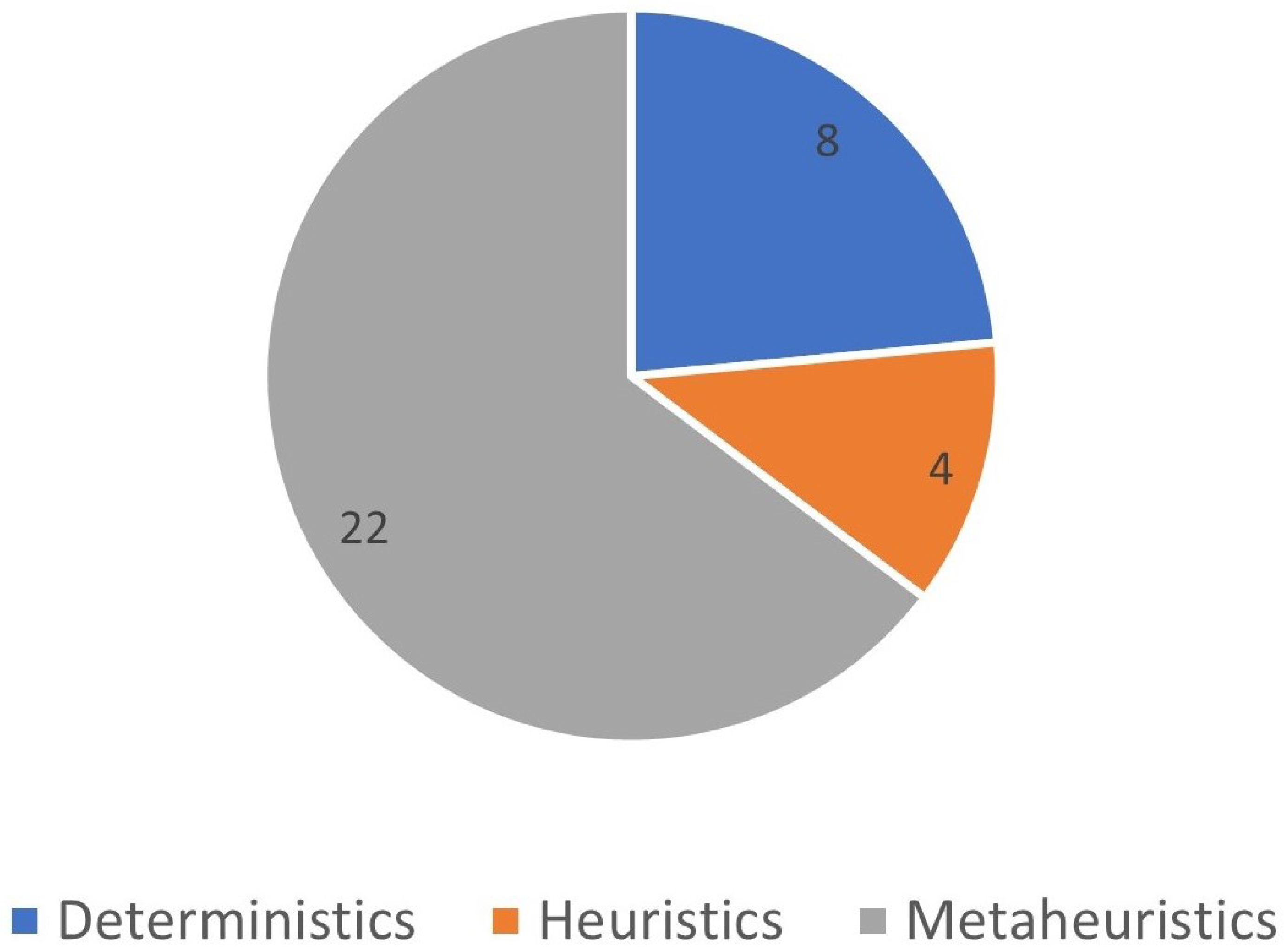
2.4. Optimization Techniques of the Inter-Array Cabling

In general, optimization problems can be tackled by using different techniques. The offshore wind farm cabling is known to be non-linear as well as non-convex; it is classified as an NP-hard problem (no deterministic solution can be found in polynomial-time) which increases in difficulty with the number of instances to be considered in the solution [20]. The non-convexity is due to the various sub-problems to be solved, possibly including the AEP maximization, CAPEX and power loss reduction, etc., so that multiple different solutions can result in the same objective value.
In the literature, various approaches have been applied for tackling cabling optimization including deterministic, heuristic, and metaheuristic methods. Deterministic approaches can guarantee finding a global optimum of the problem but very quickly become a large computational burden once the number of considered instances increases. Heuristics and metaheuristics come with more flexibility, due to, in theory, the possibility to consider all the complexity of physical modeling, at the expense of not having an optimality guarantee [5]. In Figure 5, the chosen optimization methodology of analyzed studies published since 2019 is shown.
It is shown that the majority is proposing metaheuristic approaches, which does not necessarily exclude the use of deterministics or heuristics, as metheuristics can also be used for creating an iterative framework as part of a nested approach (more in Section 2.4.3).

2.4.1. Deterministics

Global optimization can provide the mathematical certification to find a globally optimal solution under certain conditions (i.e., the need for assuming convexity) and has been applied to some extent to overcome the cabling problem [28]. Types of models useful for solving the cabling layout are binary integer programming (BIP), mixed-integer linear programming (MILP), mixed-integer quadratic programming (MIQP), and mixed-integer non-linear programming (MINLP) [29]. Compared to the other models, MILP formulations are generally computationally more efficient and are therefore the preferred choice. However, each model comes with certain limitations on how to model important engineering constraints (e.g., the quadratic active power losses can not be fully considered in the MILP model and also the widely used Newton–Raphson method to model power flow equations can not be applied in an MILP nor MIQP) and it is often not feasible to fully describe and solve the problem in an analytical form without significant simplifications of the search space [30]. Common simplifications, for example, are that the position of the OSS is restricted to only a few discrete candidate locations and that the use of cables is restricted to only a few different types in order to keep the number of binary variables below a certain threshold with which the problem will still be computationally tractable [28]. Hence, the main challenge for using deterministic solution methods is to find a reasonable balance between functionality (i.e., performance) and complexity [29]. The solution of those problems is often obtained using external solvers which are usually used as a black box, using algorithms such as branch-and-cut or Benders’ decomposition. Searching for a proven optimal solution under all combination possibilities makes the approach more transparent [5]. However, since only one solution can be obtained at a time, the solution would have to be discarded and the problem reformulated in case a solution is found to be infeasible due to an unconsidered engineering constraint [28].
With discrete decision variables they mostly solve the problem by using a mixed integer linear programming (MILP) approach and focus mostly on the radial structure ([21,29,31,32,33,34,35,36]) while only some explore the optimization of the more reliable looped structure ([30,37]). It is also the latter two articles in which the mathematical optimization program is embedded in an iterative framework called Progressive Contingency Corporation, which can simplify the problem while still including the global optimum [37]. Both papers also incorporate a stochastic model in order to analyze the impact of failure rates and MTTRs on the availability of the wind farm and hence on the EENS. Comparing radial and looped structures, Pérez-Rúa et al. [30] find that the profitability of either topology type is heavily dependent on the project size and wind turbine ratings, as these largely affect the EENS. Furthermore, it is stated that the stochastic model comes with low tractability which especially affects large-scale instances with an increase in the required computing time and memory resources.
As already mentioned, MILP models can not incorporate the quadratic electrical losses in the cables in their objective function. To overcome this issue, most authors propose a pre-processing step in which the losses are pre-computed in the form of a database which can then be accessed during the optimization process. Shen et al. [21] simplified the calculation even more by assuming a coefficient for the power loss over the OWF’s lifetime. Marge et al. in [35] use a simplification developed in [38] in which a layout is first designed without taking the energy losses into account. Then, the losses for the designed layout are approximated by the probable power flow and the cable resistances. Based on this, local modifications (e.g., changing a cable type) are made to the current layout, and the algorithm is run again until no more changes are due.
Their work ([35]) is also the only studied article that incorporates different WT layouts in a deterministic optimization. In a first step, different layouts are designed with the help of the Jensen wake model considering different wind speeds as well as directions. The WT layouts are grid-based and differ in the distances between WT rows which are then integrated into the MILP model. Although the positioning of the WTs is not directly optimized, this approach enables a broader optimization. Furthermore, the obtained power for each turbine under the influence of the wake plays an important role in the assessment of power losses and the EENS due to failures of components which are typically only considered assuming the rated power of each WT.
Most works only take into account a flat homogeneous seabed which makes it possible to only consider the Euclidean distance between two WTs. Klein and Haugland in [33] present an MILP model in which segments of different cables are allowed to share a common trajectory but are not allowed to cross paths. Cables can be placed in close proximity to turbines they are not connecting to, which is accomplished by introducing so-called “Steiner points” in arbitrarily small circles centered around the locations of the turbines to which the cables may be connected (see Figure 6).
A similar procedure is used for (multiple) cables routed around possible restriction zones on the seabed. Klein and Haugland point out that the potential cost savings can be considerable when considering the high cost per meter of cables in offshore wind farms.
Even though their MILP model proves to have a practical and applicable computational performance handling around 60 WTs, it is pointed out that it would be a challenge to adopt the model and algorithm to handle commercial-scale offshore wind farms with possibly 200 or more turbines.
This points towards the main problem that comes with the use of deterministic models, as their complexity and search for optimality grow exponentially with the number of considered instances such as WTs, OSSs, cable types, etc.
Ulku and Uslu [36] developed an MILP model to find the optimal location for a voltage source converter across the map to achieve the most cost-effective design for power transmission to the onshore substation. They limited the computational time to two hours and were able to find optimal solutions for several layouts with up to 20 fixed turbines. A higher turbine number led to non-optimal results within the given computational time. Newer works incorporating MILP models were able to increase the number of considered WTs to around 100 ([29,30,31,32]), but do not consider certain key constraints such as obstacles or no-cable crossings and furthermore suffer from long computational times compared to heuristics and metaheuristics, which are assessed in the next subsections.

2.4.2. Heuristics

Due to the intrinsic complexity of the problem and the large number of constraints, heuristic methodologies offer an efficient alternative. Heuristics can be defined as solver-free algorithms which construct a solution by following a set of sequential steps, which are based on stochastic searching processes. Hence, they offer more possibilities for pursuing better results in a shorter amount of time but could deliver unstable outputs as well as fall into a local optimum as they do not discover all of the search space [14]. In contrast to deterministic methods, heuristics alone can not be guaranteed to find an optimal solution (let alone a feasible one), but are very useful for obtaining an approximate solution within an acceptable time for NP-hard problems [16]. This is often required because the recurring process of calculating the evaluation function when simultaneously solving multiple layers of problems is often bound to a given time limit. The faster the heuristic performs, the more exhaustively the search space can be explored [2]. Classic heuristic algorithms which find application in the inter-array cabling problem are Prim’s ([24,39]), Dijkstra’s, Kruska’s, Clark and Wright’s savings ([22,23,40]), or Esau-William’s ([29]) algorithms (it is pointed out that the named algorithms intrinsically all obey the same underlying rules during the design process [41]) but also new and individual heuristics can be used as their development and integration are subject to the designer’s creativity [5].
Combining heuristic approaches with deterministic optimization can have the benefit of limiting the search space for deterministic methods which can result in an acceleration of convergence when searching for a global optimum. The merging of both methods is called matheuristic [5].
After Ulku and Uslu’s MILP formulation in [36] failed to provide optimal solutions in a two-hour timeframe, the authors incorporated heuristics in a later work [34]. Matheuristics led to faster convergence and thus reduced the computational time significantly by 55%.
Pérez-Rúa and Cutululis [2] focused on the simultaneous optimization of the OWF layout and inter-array cabling. After generating a layout by an external model taking wake and wind variability into account, it is firstly assessed in terms of cabling optimization by the Esau–Williams greedy heuristic. The authors claim that the Esau–Williams heuristic has consistently performed better in terms of feasible points and investment cost in the testing phase when compared to Prim’s and Kruskal’s algorithms. After the connections have been assessed, one out of three available cable types has to be assigned to the WT connections. This decision is made by evaluating the number of downstream turbines connected to the branch and choosing the cheapest type capable of handling the given capacity. After assessing the objective value (here the internal rate of return), a random WT is randomly moved and the process starts again. This is repeated until a certain time budget has run out. The best preliminary solution is taken forth to a global optimization with an MILP which can now solve the cabling for this specific layout optimally, taking pre-processed power losses into account as carried out in their previous work [29].
The MILP model in the upper example provides optimality to the cable type selection for each WT interconnection. Routing heuristics alone can not decide on an adequate cable type for WT interconnection, hence this is mostly carried out in a subsequential step. To overcome this, Zuo et al. [24] deeply modified Prim’s algorithm to foresee which possible connections may follow so that during the heuristic run, a feasible cable type can already automatically be selected. This way, a higher control is achieved, especially in terms of keeping track of the number of feeders for the OSS and the number of turbines per feeder.
Another example of how heuristics can speed up an iterative design process is shown in [23] as well as in the follow-up work [22], in which a large offshore wind farm is partitioned and the cable layouts in different regions were optimized. What is special about this work is that it focuses specifically on the inter-corporation across OSSs, adding another level of redundancy to the cabling structure (illustrated in Figure 7). Furthermore, it is argued that by connecting the two OSSs, a transformer sharing capability is established, which reduces the acquisition cost of spare parts. After two substations have been positioned in the OWF by clustering methods, iterative angular adaptations (and thus stepwise changes of the WT allocations) are used to establish the cabling between the OSSs and the WTs by Clark and Wright’s savings algorithm.
Gong et al. [40] investigate (in a simple manner) the construction of a new, more reliable cabling structure. It should be noted that they, unlike most works, consider a heterogeneous seabed and use the geodesic length based on triangular meshes of the seabed to compute exact lengths between WTs. They first explore a ring structure which is partially redundant but can still (due to only one available cable capacity with n turbines) suffer from overloads if a failure close to the substation occurs. After locating the OSS in the center of the OWF, they allocate the 2n − 1 WTs to feeders using the sweep algorithm. To find the optimal routing for this feeder, the savings algorithm by Clarke and Wright is used. This procedure optimizes the use of the cable capacity and naturally reduces the occurrence of forbidden cable crossings. Based on the ring structure, they introduce the reliable “multi-loop structure” (see Figure 8). Additionally, it uses WTs in those ring structures as nodes to connect to other rings. To find those nodes, the turbines in each feeder are counted up to the (n + 1)-th turbine which is identified as the interconnecting node. When all interconnecting nodes have been found, the sweep algorithm is applied and interconnecting nodes that are swept will be connected to the next-swept connecting point.

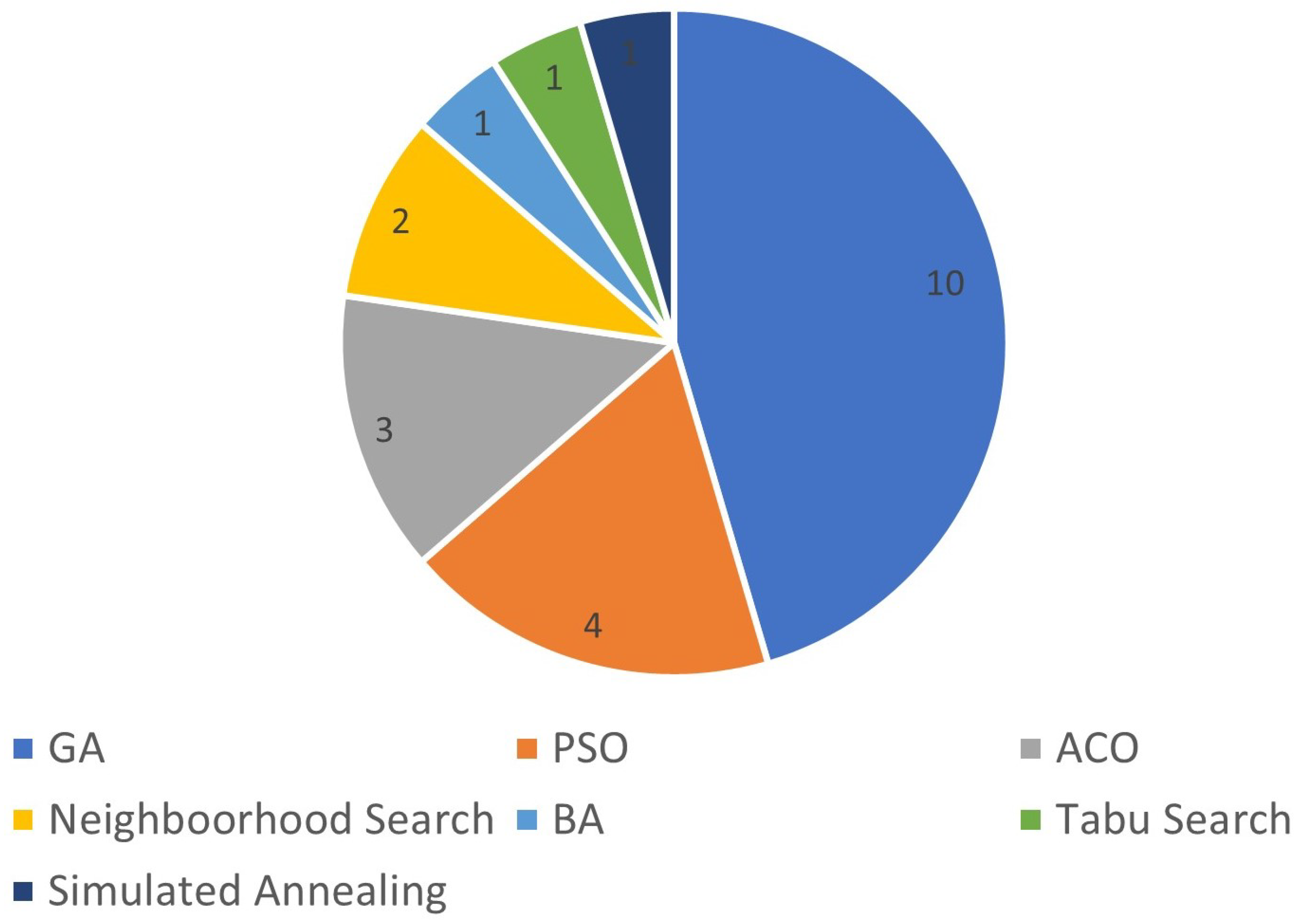
2.4.3. Metaheuristics

Metaheuristics are generally used to guide the search process with the goal to find near-optimal solutions while exploring a large-enough search space without being too computationally expensive. Their use is more typical when an initial solution is intended to be improved in an iterative manner in a nested (3) approach (see again Section 2.3). Metaheuristics make use of different stochastic operators in order to enhance traditional heuristic algorithms, i.e., to avoid them from falling into local minima by smartly searching a larger search space [5]. These methods are mostly based on naturally occurring phenomena such as (but not limited to) the genetic algorithm (GA), the particle swarm optimization (PSO) algorithm, the ant colony optimization (ACO) algorithm, the bat algorithm (BA), neighborhood searches, tabu searches, or the simulated annealing algorithm. An overview of the published work since 2019 is given in Figure 9.

Genetic Algorithm

The GA is named after principles observed in evolutionary processes to create and test new solutions. For reasons of clarity, a short description is given in the following based on [42]: An initial population consists of multiple individuals with individual chromosome pairs, e.g., one individual’s chromosome contains specific information about the OSS location for this specific individual’s solution. Every GA generation begins with a selection, where pairs of individuals already in the population are chosen based on the quality of their solutions to provide genetic material for the next generation. These pairs of individuals are combined using crossover and mutation operators to produce new solutions, called child solutions. These child solutions take on some of their parent solutions via crossover and are then modified, possibly randomly, via mutation. Using these two stochastic operations, GAs try to preserve the good elements of the parent solutions in the new child solution, while the random element is used to avoid settling in local optima solutions. The “replace the weakest first” strategy is then utilized to determine which of the newly created children will be included in the next generation. This process of selection, crossing, and mutation is repeated until a certain portion of the population has been replaced and the quality of the entire population has improved, marking the end of a generation. Generally, GAs continue for a predetermined number of generations or until there is sufficient similarity (i.e., convergence) in the population. Although both crossover and mutation take constraints into account, after crossover and mutation, constraints are explicitly imposed and if a child solution does not satisfy a constraint, crossover and mutation are repeated until it does.
For the inter-array cabling of OWFs, GAs can be used in two ways. The information about the electrical system (e.g., OSS locations, WT interconnections, cable types, etc.) can be integrated into the chromosomes, so that each individual represents a different and complete cabling solution [43].
Another method used in the literature is to use the chromosome information to only contain parts of the overall problem (e.g., WT positions, the OSS location) while the rest of the connection (e.g., WT allocation, cabling) is carried out using non-metaheuristic approaches, i.e., clustering or cabling heuristics, respectively, in an iterative nested approach ([13,14,16,17,44]).
From the works studied using GA, only three investigate the construction of the more reliable ring structure ([13,14,45]). The latter compares radial and ring structures in terms of life cycle cost including unavailability and repairs while ignoring power losses over the OWF’s life time. It is concluded that partial redundancy of the system can outperform full redundancy compared to the radial structure since the CAPEX is increasing with the level of redundancy. With their specific cost assumptions, partial redundancy is economically more viable after eight years of OWF operation while amortization is reached after twelve years in the total redundancy case, leaving the radial structure as the most expensive after the OWF’s lifetime. Only considering the cabling CAPEX but therefore taking lifetime power losses into account (at nominal power production), Wei et al. [13] also compare ring and radial structures and come to the same conclusion that the ring design is more expensive, but, with the same failure rates, is more economical in the long term. It is interesting to note that the authors decided to use a single-parent GA, as they point out that this would lead to faster computational times.
A very sophisticated power loss model is introduced in [43], where a variable wind speed is considered for calculating the wake losses inside a fixed OWF layout and to determine the power output of each individual WT. They also consider current and voltage drops in each branch. WT interconnections, cable types and possible OSS positions are contained within the chromosomes and are all simultaneously optimized considering the fitness function of CAPEX and power loss cost. For creating a new generation, adaptive niche techniques are utilized to maintain population diversity and avoid local convergence. They report that this procedure comes with significant cost reductions when compared to the sequential step approach in which first the cabling length is minimized and subsequently the cable type is selected.
GAs can also be used to position WTs effectively in the OWF either in a grid-like ([46]) or coordinate-based ([44]) layout. Both works only consider one cable type and therefore only try to minimize the overall inter-array cabling length. Wade et al. [44] make use of two heuristics, namely the planar open savings heuristic (developed by Bauer and Lysgaard in [47]) and the Esau–Williams algorithm.
In [46], a Euclidean minimum Steiner tree (EMST) approach has been explored, utilizing a “GeoSteiner” algorithm solver which is an exact algorithm to solve the EMST problem [48]. Compared to finding an MST according to the fixed vertices, an EMST allows to add extra vertices to the network in order to reduce the overall length, as illustrated in Figure 10.
With this method, a solution for a small problem (about 30 turbines) can be generated in less than an hour; however, for a larger problem (about 50 turbines), the calculation time increases rapidly to about 10 h. It should be noted that this work did not incorporate any OSSs in its model.
Considering a heterogeneous seabed, Yi et al. [20] divide the available seabed area into different zones. These correspond to different cable costs in order to penalize solutions in which cabling would be more complicated. Furthermore, exclusion zones are considered where cabling is not permitted. To cope with the exclusion zones, a visibility graph is constructed before the cabling problem is assessed. This graph contains all connections from the starting point (OSS) to all straight-lined accessible clients (WTs), the corners of the exclusion zones, and their edges. For reasons of clarity, a visibility graph is included in Figure 11 from [9], where this problem is also tackled accordingly.
For the initial solution, Yi et al. [20] use a stochastic greedy run which assures connectivity of all WTs. After the initial connection is set by 500 greedy runs through the visibility graph, the GA randomly chooses branches for re-connection. The turbines in this branch are then connected to their nearest connected neighbor WT. If the solution provides better results, it is taken forward; otherwise, the move will be discarded. It is worth noting that the used model is relatively complex considering 119 WTs, 2 OSSs (by K-means clustering) in 5 different installation zones, power outputs (and correspondingly electrical losses) due to wake effects, and availability accounts due to stochastically occurring cable failures.
Furthermore, considering the installation complexity of certain seabed areas, Roetert et al. [49] are the first to consider morpho-dynamic seabed conditions in the cable route optimization problem. Their work can be divided into two parts. Firstly, they develop a GA to find the optimal turbine interconnection considering a static seabed. Herein after, they optimize these gained connections by varying the cable’s vertical (initial burial depths) and horizontal offsets to avoid cable exposure due to seabed movements in the form of migrating sand waves. In the GA, the initial population consists of multiple solutions for the layout problem. An initial solution consists of one string containing all turbines in a random order which is infeasible but denotes turbine connectivity. For each solution, the total weight is calculated by adding up all edges present in the solution. For every possible connection between turbines, as well as turbines and the OSS, a certain “weight” according to seabed restrictions is generated and saved in a distance matrix. In a second step, the total population is divided into sets of eight solutions. With a sufficiently large population and a division in subsets, the risk of local optima being considered globally optimal is diminished. Later on, the fitness of all solutions is evaluated by assessing whether all turbines are connected to the OSS and whether the string capacity is exceeded. The solution with the lowest total weight is then chosen as the best solution in this set. The fourth step consists of applying eight mathematical operations independently to the best solution in a subset. This repeats until a certain maximum amount of computational time, a specific number of iterations is reached, or no significant improvement in the total solution can be identified. With the aid of the GA and the constraint of non-crossing, as well as defining a maximum number of turbines per string, a somewhat optimal layout is calculated. The gained connections are then subject to variations in vertical and horizontal offsets. Internal and external risks are analyzed and are included in the cost function as well as the required burial depth for each possible hazard. The vertical determination is achieved by sectioning the connection and varying the burial depth per section. Then, for each section, the optimal initial burial depth in terms of minimized cost is determined and all segments are combined. Independently, the horizontal offset is determined by the use of Dijkstra’s algorithm which searches for the shortest path between two given vertices for a graph with weighted edges. It can be observed that the more cost-efficient parts are located in the sand wave troughs, since they already represent the lowest seabed level where the predicted seabed lowering is equal to the uncertainty band.

Particle Swarm Optimization

Like the GA, the particle swarm optimization (PSO) algorithm is a population-based metaheuristic optimization algorithm. It is inspired by the collective behavior of social animals. Within the PSO, the set of candidate solutions to the optimization problem is defined as a swarm of particles that can move freely in the multi-dimensional search space, defining trajectories. Each particle updates its position in each iteration of a loop based on its personal best solution found so far, the global best solution found so far by all particles, and according to its velocity of the subsequent iteration. This is expected to move the swarm towards the best solutions [50].
Similar to the application of GAs in the inter-array cabling, the metaheuristic information of a PSO can be used in two ways, while works incorporating GAs mainly focus on providing the framework for other heuristics (e.g., OSS or WT positioning) to conduct the inter-array cabling in a nested approach, PSOs are mainly used to optimize the IA cabling ([51,52]) or OSS position ([40,53]) or even both simultaneously ([54,55,56]).
Pillai et al. [18], on the other hand, developed a nested approach that is iteratively run by each particle solution in which the WT layout, OSS position, and IA cabling are optimized simultaneously. The WTs are positioned taking the wake effect into account considering variable wind speeds and directions. With the initial WT positions, one OSS is positioned using K-clustering while the inner grid cabling is handled afterwards by an MILP model. In subsequent steps in the PSO loop, the AEP and the LCOE as the fitness function are calculated, respectively, taking into account the initial investment cost, electrical losses, and the cost for decommissioning. The cables are assumed not to be recovered. After each particle ran through the loop, the particles are re-positioned in the search space, corresponding to new WT layouts. All steps adhere to the implemented seabed conditions, meaning that no WTs, OSS, or cables can be placed in certain zones in the wind farm. This is carried out by introducing a Delaunay triangulation which is an approximation of a visibility graph explained earlier (see again Figure 11), which was already used in their earlier work [57]. For an explanatory illustration of the Delaunay triangulation, please refer to [57]. The PSO loop is repeated until the population diversity is lower than 10%, which indicates a settlement in the global optimum.
Related to the Delaunay triangulation mentioned above is the use of a Voronoi diagram which was implemented by Qi et al. [51] to prescribe the WT connections. In the K-shaped Voronoi diagram, according to the nearest neighbor rule, each discrete point is assigned to the area of the vertex to which it is nearest so that each discrete point corresponds to only one region as illustrated in Figure 12. It can be observed that the Euclidean distance between OSS node 1 and WT node 6 is closer than the distance 13 ¯ . However, node 3 is a first-order neighbor to the OSS. Hence, this connection is preferred. As this avoids cables crossing adjacent areas without connecting to any node, the probability of cable crossings is automatically minimized.
An adaptive particle swarm optimization with local search is implemented in order to optimize the cable routing for a fixed OWF consisting of multiple WT types with different rated power values. The local search randomly changes a value of one dimension of the global optimal position particle. If this move benefits the global best, it will be accepted; otherwise, it will be randomly re-executed until a limit is reached. The integrated local search enhances the algorithm’s searching ability and can improve the heuristic solution significantly. The fitness function consists of the CAPEX for initial cable installation but also takes the energy losses due to cable resistances over the OWF’s lifetime into account. By considering the cable’s quadratic energy losses in the fitness function as well as the cable type, they prove that, in the long run, it is heavily beneficial in terms of cost to choose a cable type accordingly, rather than selecting the minimal possible cable type and, hence, it is conducive to reducing the total cost of OWF during the operational period.
Qi et al. [51] are the first ones to incorporate Voronoi distances into the cable connection layout optimization problem and show by comparison with a PSO algorithm working with an MST designed in [58] that the Voronoi distances are better suited to judging the proximity relations between points in the layout.
The impact of considering cable losses on the cable selection is also highlighted in [54], where it is reported that the energy (and therefore the current) supported by the cables is generally overestimated when not taking wake effects into account. This leads to a larger cable selection and therefore higher cost. Cost savings of up to 1 3 are reported. Although the authors make use of a simplified energy loss calculation (the Newton–Raphsom load flow method), computational time increases ten-fold when considering the power losses in the cable type selection process compared with taking the rated WT power into consideration.
In [52], two metaheuristics are applied to solve the overall OWF layout model. In an outer layer, a GA designs the layout when given OWF parameters such as area, available WT types as well as prevailing wind speeds and directions. Hence, the algorithm decides on a near-optimal OWF capacity which is normally a strict input. With an initial layout and an OSS fixed to the OWF’s center, a binary PSO (originally developed by Pookpunt and Ongsaku in [59]) is conducting the IA connection scheme and cable type selection. Since the authors explore the interaction of wake and different turbine types, they conclude that due to wake-induced different wind resources in the wind farm, a combination of different types of WTs can be beneficial in order to satisfy the requirements of both high average capacity factor and low variance in power production.

Ant Colony Optimization

Ant colony optimization (ACO) is another population-based metaheuristic that mimics the behavior of ants when randomly looking for food and leaving a trace of pheromones along their paths. When a food source is found, the ant returns to the nest and thus increases the pheromone concentration on that particular path. The other ants notice this and tend to follow the paths with the highest pheromone density. In this way, the paths leading from the anthill to a food source are reinforced. However, every ant is equipped with an individual susceptibility to the pheromone concentration found, which is part of a local search strategy in order to possibly discover new paths. Due to the initial random fluctuation, the shorter paths are preferred because the ants return to the nest earlier and the pheromones have less time to fade than those on the longer paths. Hence, a vital parameter for building the metaheuristic is the pheromone decay probability which is used to calculate an edge’s probability when exploring the search space. It needs to be large enough to allow “wrong” edges to be forgotten, especially if chosen in the initial stages of the algorithm where the solutions are more or less random but not too strong to delete the previous “good” edges found in good solutions [27].
Two studies have been analyzed with a focus on the application of ACOs for the IA cabling problem ([19,60]).
In [19], 133 WTs are randomly positioned, followed by K-means clustering which positions four OSSs in each cluster center. In each cluster, ants are distributed randomly on WTs and each WT is visited once by every ant during a random walk. The shortest paths will have the highest amount of pheromones. As a local search step, the ant’s likelihood of following pheromones is adjusted. However, they point out that pheromones on most favorite paths do not change much, which leads the ACO to converge to a local optimal solution. To help the ACO discover new solutions, the four-vertex three-line inequality heuristic is adopted as a local search strategy. If that does not improve the solution, Prim’s algorithm is applied in each cluster. The final layout is visibly not implemented in practice. Each of the four OSSs is only fed by one cable which radially collects the energy from each turbine. Furthermore, Wu and Wang [19] stage a main substation in the middle of the wind farm which collects the energy from the cluster OSSs, and their interconnections cause multiple cable crossings. No export cable is considered.
Taylor et al. [60] compare the MILP model (previously developed in [61,62]) with a newly developed ACO. For the original MILP model, due to computational constraints, power losses based on the power curve (depending on wind variability) of each WT have been pre-processed, which is also carried out for the ACO in order to obtain comparable results. The OWF layout consisting of 112 WTs and two OSSs is fixed and only the cabling is optimized. Three available cable types are considered, and type selection is based on the lowest acquisition cost.
The ACO starts with placing an ant at the furthest-distanced (unconnected) WT to the OSS, which, from there, starts “randomly” visiting nodes until it reaches the OSS. Another ant then starts at the next-furthest (unconnected) WT, and randomly visits nodes until it reaches a substation node or a turbine on an existing string. This procedure is repeated until all WTs are connected (in a possibly unfeasible manner). Now, the fitness function can be evaluated. It is worth noting that several penalty functions are implemented, which restrict unfeasible solutions to be taken as global bests. In essence, cable crossings are penalized as well as the crossing of exclusion zones which are modeled by Steiner points. Furthermore, the authors restrict the number of feeders connected to the OSS. According to the fitness function, the pheromones on each path that led to the global best solution can be updated. The algorithm is then launched again, eventually converging to a near-optimal solution which is 0.4–7.6% worse compared to the MILP model while not suffering from the same memory and time constraints as the MILP algorithm.
However, certain problems have been discovered when updating pheromones of the global best solution since the pheromones are equally distributed on all branches which have been utilized (while obtaining the global best), not taking into account that there can be connections involved which would have worsened the obtained solutions if others did not enhance it. Hence, a decomposition into sub-problems (ACOsp) is adapted in the form of a post-processing step of an obtained solution. Two branches are randomly selected and their connectivity is discarded, while all other branches stay unchanged. In this unconnected sub-region, the ACO is launched again, while the fitness function is evaluated for the whole OWF as WTs in the sub-region can be connected to already-connected WTs outside the sub-region. Once all branch pairs have been evaluated, the same is conducted for sub-regions consisting of three branches which further increases the size of the search space.
The found solutions cost only 0.0–1.4% more than optimal solutions. However, for the largest case with 122 WTs, the computational time is approx. eleven-fold compared to the classic ACO but 2 3 of the computational time needed by the MILP algorithm.

Bat Algorithm

The bat algorithm (BA) is inspired by the preying process of bats using echolocation. Depending on the distance to their prey, bats vary the utilized wavelength and frequency of the firing pulse. This can be adopted to solve optimization problems as is explained in more detail in [63] by creating a population of bats and iteratively changing their behavior based on personal experiences, but also based on the collective search quality in the search space similar to the PSO.
Qi et al. [64] make use of this to solve the inter-array cabling for 50 WTs in an irregular fixed layout with a predetermined OSS location.
Iteratively, the positions of each bat in the population are updated by varying their velocity and frequency, mutation, the bat’s loudness, and emission frequency. The bat’s position contains information about cable layout as well as the available cable types.
To enhance the algorithm’s local search ability, they introduce a varying operator which inserts a bat’s position into another bat’s position. To trigger this varying operator, they use the bat’s previous behavior, i.e., its pulse loudness and emission frequency, which are designed to balance the global searching ability and the local searching ability of the BA.
In their case study, the authors compare different approaches based on the chosen cable selection scheme, i.e., (I) where the thinnest (most cost-effective) cable that satisfies the cable current constraint is selected or (II) where the impact of the cable selection on the objective function (hence on the power losses) is considered while allowing crossed cables. Approach (III) is based on (II), but penalizes crossings significantly. In the first scenario analyzed, 11 cable types are considered and it is found that approaches (II) and (III) are producing similar total costs which are 2% lower than the results obtained by approach (I). Due to the prior restriction, the minimum cable selection approach already converges after 120 s. However, the most realistic approach (III) also converges relatively fast after 250 s of CPU time, which indicates the general feasibility of the BA in the IA cabling optimization.
Due to the high production volume related to eleven cable types, a more reality-based scenario is performed with only five available cross-sections. With a lower amount of available cable types to choose from, the accuracy of approach (III) becomes more or less obsolete, because the chosen minimum cable is now more likely to support even more turbines, which lowers electrical power losses automatically. Hence, the purchasing cost is more likely to unnecessarily increase just to save more electrical power losses. Computationally, all approaches take longer to converge now at the same time at around 350 s.
It can be concluded from this study, that the number and segmentation of available cable types significantly influences the suitability of different approaches.

Neighborhood Search and Others

Cazzaro et al. [27] have tested five different metaheuristic schemes in a case with 220 turbines with fixed placements and one substation with three previously determined possible positions. The algorithms tested are GA, simulated annealing (SA), ant colony optimization (ACO), tabu search, and the variable neighborhood search (VNS). The heuristics are explained shortly below. Since the case with 220 WT is rather large, their first approach is to utilize the SWEEP algorithm (see again Section 2.3) to find good initial solutions which can be used for the other metaheuristics explained shortly below based on [27].
Simulated annealing comes from re-heating and cooling of metals in order to get rid of impurities by lowering the energy in the system (here the solution cost). Originally, the main parameter is called temperature and it is updated at each step controlled by a parameter describing the cooling speed. Another important feature of SA is the probability of accepting a move, which favors the procedure of passing from one solution to another. One move is always to accept when an improvement in terms of energy of the solution is possible. A move is allowed for a worsening with good probability only when the temperature is high and the acceptance probability must depend on the magnitude of the difference between the energy of the candidate move and the energy of the current solution.
The tabu search works with a memory structure called tabu list that registers which moves the algorithm is not allowed to repeat (for a while). This allows the metaheuristic to reach new solutions while avoiding returning to a previous local optimum. There are three options that the tabu list forbids: nodes where the connection is coming from; nodes to which the connection is going; newly chosen arcs can not be removed too soon. It was shown that the third option is the most efficient.
The variable neighborhood search (VNS) consists of three main steps, which are repeated until a time limit is reached. Only one parameter, k, is needed which describes the current neighborhood considered in the set of neighborhoods. This makes VNS easy to adjust. The first step is “Shaking” where from the initial solution obtained by SWEEP, random k arcs are changed in the k-th neighborhood. Secondly, a local search is applied to find the best arc change until the solution cost stops improving. Afterwards, it will be decided if the overall solution has been improved; if not, the initial solution is kept and the next neighborhood is considered. If an improvement can be made, the new solution is saved and the neighborhood counter is reset.
Cazzaro et al. [27] found out that the tested metaheuristics are capable of increasing the initial SWEEP solution by only 4–5%. The overall best performance was achieved by VNS reaching the best solution among all metaheuristics in over 92% of all cases. In the rest of the cases, VNS was outperformed by tabu search but only by a small margin. The tabu search performed second best with a gap to the VNS solution cost of less than 2%. A possible explanation is that the local search allows the VNS and tabu search to reach good local minima while simulated annealing and the genetic algorithm seem to arrive close to good solutions but struggle to reach the global minimum. The GA is able to improve the initial SWEEP solution only in about 20% of the cases. Besides the missing local search phase, this can be explained by the fact that the internal mechanism of the GA is more complex and requires heavier computation per generation. The ant colony optimization even struggles with reaching feasible solutions since it tends to just connect a few cables to the OSS (anthill) which are not able to support all the power produced by the wind farm.
Based on the experience described above, the same authors focused on the neighborhood search metaheuristic in a later work [9]. They note that the branched topology problem has only been studied in an unbalanced case, meaning that an arbitrary number of WTs could be allocated to a string, resulting in strings carrying different amounts of electrical charges. The main disadvantages of this asy224 etrical routing are the additional cost of the electrical equipment (i.e., a spare offshore transformer module) that must be installed in the offshore substation, whereas balanced cable routing allows a single type of transformer to be used as a spare. Therefore, Cazzaro and Pisinger [9] point out that the industry prefers the balanced option although it might result in longer cabling.
To further enhance reality-based modeling, they consider obstacles in the wind farm layout by utilizing a visibility graph (see again Figure 11) now interfering with the well-suited SWEEP algorithm. Hence, they adjust the SWEEP algorithm following the shortest visibility paths and perform SWEEP at the string end for each turbine. The initial solution undergoes several operations (neighborhoods) with increasing complexity before the final solution is output. After each operation, the WT’s interconnection in each feeder area is solved optimally by brute-force enumeration or the application of MILP models.
Firstly, they swap two WTs in neighboring branches, followed by a cycle swap consisting of an exchange of multiple WTs among branches. The double swap operator exchanges two pairs of turbines at the same time between three adjacent root branches while in the following re-partition operator, two adjacent root branches are selected and completely re-partitioned and re-routed.
Comparing the branched and the radial topology shows that the radial topology is only around 1.4% more expensive, which underlines the industry’s choice to use radial connections, which require fewer electrical components than the branched solutions. However, the runtime of the optimization is three-fold when investigating the radial structure. It is shown that the biggest improvements are made after the first phases and that the double swap is the most time-consuming, accounting for half of the optimization.
Comparing the developed metaheuristic to an MILP model for an unbalanced case in [61], the worst case is 0.60% more expensive than the best-known solution while the average runtime can be decreased from 700 min to 5 min.

2.5. Comparison of Methodologies Used in the Literature

Even though deterministic models guarantee finding an optimal solution for offshore wind cabling optimization problems, their computational time increases significantly with the number of considered instances (at least with widely used computers nowadays). This problem will be encountered more and more in the future as OWF sizes tend to grow. Several authors have encountered that problem and have therefore pledged for the use of heuristics if OWF sizes grow over a certain threshold. It must also be considered that most authors using a deterministic model have solely focused on the optimization of the electrical layout and have not taken into account the overall optimization of WT and OSS positioning together with the electrical grid. With more systems to consider, more variables and constraints will need to be incorporated into the model which makes it even more time-consuming. Especially problematic is the common neglect in the literature of the natural non-convexity of the problem which makes the development of widely used MILP models possible in the first place.
Prim’s widely used algorithm is a fairly easy procedure to identify an MST in a layout with fixed nodes. It is able to find an optimal solution if only one type of cable and no constraints other than connectivity are considered. Solutions found in more complex problems were often infeasible because the few arcs connected to the OSS each had to support a large number of turbines, but were technically not able to carry that amount of capacity. Likewise, Cazzaro et al. [27] point out it can be used to find an initial, but probably infeasible, solution for other metaheuristics. By considering the cheapest cable for each edge in the MST and ignoring the fact that the power may exceed the cable’s capacity, the solution to Prim’s algorithm can provide an approximate lower bound on the cost of the optimal solution.
Furthermore, Clarke and Wright’s savings heuristic is frequently used and can be used for cabling layouts where loops are intended. However, it does not include strategies for avoidance of cable crossings, which can be a major concern in feasibility regarding installation and O&M activities [40].
Population-based metaheuristics such as GA and PSO are widely used in the offshore wind optimization field. As with all heuristics, by nature, they do not guarantee finding the optimal solution, especially for a complex objective function such as, e.g., the LCOE, since they involve a risk of premature convergence but show good performance in solving non-convex problems. Since methodologies based on the genetic algorithm explore a very wide solution space, they are able to search for good and feasible solutions, but therefore require a major computational effort [17]. In order to accelerate the rate at which the process and its ability to avoid local solutions converge, Srinivas and Patnaik in [65] proposed the use of adaptive parameters such as mutation and crossover. Pillai et al. [66] have implemented these adaptive operators in terms of probability functions of the quality of the solution. The solution’s fitness value is therefore compared to the population’s mean fitness value so that better solutions not only have a higher probability of being selected, but also have a higher probability of contributing through crossover effects. Another option in order to enhance the quality of the solution is to use single parent mutation operators which, according to Wei et al. in [13], can guarantee that all the new individuals have feasible solutions. It also can improve the ability to search the solution space since any parent can produce the new individual with a limited amount of “gene” exchange, which contributes to a higher convergence speed.
The main difference between PSO and GA is the fact that PSO is based on swarm intelligence, which leads to the promotion of a cooperative environment where individual decisions directly influence each other, while the genetic algorithm is seen as a competitive metaheuristic where different solutions compete for survival [18]. All particles in the PSO are therefore aware of the improvements found by other members of the swarm and are able to adapt that information to their own movements in the search space. Keeping that in mind, it does not seem surprising that different benchmarking studies have come to the conclusion that PSO is more likely to find high-quality solutions in less time than a similar genetic algorithm which needs more parameters to be adjusted (e.g., [67,68]).
Considering the ongoing wind farm growth and the new complexity and constraints for the development of future wind farms, PSOs, but also currently less-used metaheuristics such as neighborhood searches, bat algorithms, and possibly tabu searches, might be of interest to wind farm developers, as these methods allow to identify more feasible solutions than industry standard multi-step optimization approaches, leading to more efficient wind farm layouts.

3. Floating Offshore Wind

Floating wind turbines can be used to harvest stronger winds farther offshore in water depths in which conventional bottom-fixed turbines can not be economically installed. The as-yet relatively nascent technology has entered the pre-commercial stage and will soon experience commercial-sized deployments worldwide.
Due to the floating nature, the inter-array cabling needs to be capable of adjusting its shape without harming the electricity flow or its connection to the floating platform. This is achieved by the use of so-called dynamic cables rising from the cable’s touchdown point (TDP) on the seabed to the cable hang-off point (HOP) on the floating structure. Different shapes can be realized with the help of buoyancy elements or even clump weights distributed over the length of the cable in order to distribute the acting forces and to be able to adjust to certain offsets of the structure. It should be noted that the design offset which is limited by the station-keeping system is due to the allowance of the dynamic cable as the electrical connection can only be guaranteed under design tensions. Since the environment is highly dynamic, the cable experiences much more stress than compared to the bottom-fixed case where only static cables are deployed. Hence, dynamic cables need protection from overbending and abrasion both at the HOP and at the TDP. Bend stiffeners at the HOP are typically used to prevent the cable from overbending while protective sleeves at the TDP protect the cable from seabed abrasion.
Common industry practice (especially in relatively shallow waters) is to connect the dynamic cable to a static cable section which is buried in the seabed and is used to cover longer distances of electricity transfer. However, due to economies of scale and the increased costs in the case of submarine joints between static and dynamic cables, having a TDP might not be economically viable as the dynamic cable could stay in a suspended position before rising again to connect to another turbine. It could also come with benefits in reliability, as fewer connections are used, reducing the number of possible points of failure. However, the suspended configuration still needs to prove its feasibility in real applications, although it is already subject to research ([69,70]). Especially beneficial will be its application in large water depths, as it would also diminish the need for costly deep-water trenching. Different cable configurations are illustrated in Figure 13 followed by Table 1 which lists more details.
As illustrated, the chosen configuration greatly impacts the overall length of the cable and thus the area of possible impact by, e.g., waves, currents, and marine growth. Contact with mooring lines should be avoided in all respects so as not to further strain the already mechanically stressed structural integrity of the cable.
As described in the bottom-fixed literature, optimizing the overall wind farm layout is key to reaching good results. However, due to the lack of industry experience, only a handful of the optimization literature regarding the layout or cabling is published. Hence, a short review is given, highlighting the need for further optimization works.

3.1. FOWF Inter-Array Cabling Optimization

In 2019, Lerch et al. in [71] first addressed the cabling optimization in FOWFs by utilizing a PSO considering 50 WTs in a fixed layout with one OSS. As a dynamic cable configuration, the lazy wave form is assumed. The particle information in the search space consists of the cable types, turbine connections, and the cumulative power to be transmitted. If the presented solution was not feasible, the particles were reallocated and checked for the lowest cost which included the cost of acquisition, installation, and power losses (based on production of individual turbines) in the cables. As often discussed, the CAPEX is highly dependent on the length of the cable. The authors assume the length of an interconnection between two floating platforms as
L I A = 2 D w × 2.6 + D F O W T s ,
where D w denotes the water depth and D F O W T s the Euclidean distance between FOWTs. As can be seen, the cable is assumed to be connected to a static part with the length of D F O W T s before it rises again to connect to the next FOWT. The factor of 2.6 is not further explained but it is assumed that it accounts for the classic wavy shape and/or for the detour the cable has to undertake to avoid the station-keeping system.
For the power production, a Jensen-based wake model is taken into account which considers single, partial, and multiple wake effects and wind directions while the individually generated power is dependent on the turbine’s tip-speed ratio in the form of power coefficient and experienced wind speeds.
The authors optimize a layout in Golfe de Fos, France, which has been developed in the LIFES50+ project, consisting of 50 FOWTs at a water depth of 70 m. The original layout only uses two IA cable types while their optimization considers six cable types to be available, which makes it less representative. They are able to reduce the total cost by 6%, and power losses and cabling length by 8%. Furthermore, the amount of OSS feeders is reduced.
In a later step, the effect of discounts due to the use of solely the two greatest cable types is assessed assuming a discount of 15%. They find that the reduced energy losses can not compensate for the higher acquisition cost at that discount. However, this is highly dependent on the available cable types.
In 2021, the authors adapted their work in [50] and introduce reliability-based EENS as well as OSS position determination from predetermined possible OSS locations taking the cost of the export cable into account. Furthermore, they adapt the cable length determination to
L I A = 1.05 D F O W T s + 2 ( L d y n a m i c D x ) ,
where L d y n a m i c denotes the length of the dynamic cable part and D x the horizontal distance from the hang-off point to the cable’s touchdown. The 5% increase in the static cable part is due to cable routing around the station-keeping system which is based on industry discussions. However, no further statement regarding the considered mooring system is made. L d y n a m i c can be determined by segmenting the lazy wave form into three catenary lines, assuming the curvature as a hyperbolic cosine function and calculating each arc length.
Regarding the reliability assessment, they only consider failure rates and MTTRs for feeders directly connected to the OSS (taken from [11] for static cables), the export cables, and the transformers.
Lerch et al. [50] validate the model successfully by comparing it to deterministic mixed-integer quadratic constraint programming (MIQCP) developed by Banzo and Ramos in [72] under the adoption of a few constraints, e.g., the allowance of cable crossings, the consideration of variable OSS locations, and the fact that the wind turbine connection possibilities are restricted to the adjacent wind turbine of its row. In comparison, the difference in required computational time for the exact same solution is immense; while the MIQCP needs 26 h for the exact calculation, the adapted PSO only takes 14 s.
Lastly, the authors compare two inter-array cabling options. Namely they compare the options of connecting FOWTs by solely dynamic cables without a specific submarine joint to static cables with the traditional use of buried static cable sections. Main difference is that the cost-intensive submarine joint would be redundant. Nevertheless, the dynamic cable would be buried to cover major distances between turbines and would therefore need extra protection which makes them more expensive. The technical feasibility of only using a dynamic cable which is partially buried is not assessed but it can be expected that this configuration will lead to large scour and bending forces on the cable’s burial points. On the other hand, having only one cable part could come with reliability benefits as less connection and hence less possible breaking points are included. However, in case repair is needed, the maintenance work will likely be much more complicated since an individual part can not be exchanged easily. However, as the optimal design is very case dependent, an universally valid statement could not be made. The option of having no touchdown point, i.e., having a fully submerged dynamic cable section between both structures is not assessed.

3.2. FOWT Positioning

In 2015, Rodrigues et al. [73] presented an optimization framework for reducing overall losses due to the wake effects in FOWFs. The authors aim to find optimal anchoring locations as well as optimal locations of the FOWTs within the allowable offset area depending on incoming wind directions. They assumed that the FOWTs could be moved in a controlled manner by using pulleys. With the help of an evolutionary algorithm, they made use of a nested approach by establishing the turbine’s three anchoring positions in an outer loop while optimizing the turbine location within the possible watch circle for each wind direction in an inner loop. The overall goal was to maximize the FOWF’s efficiency (calculated ratio between wind farm production with and without wake losses, which is computed as mean power output for all wind directions and scaled according to each direction probability). At all times, the minimum distance of two adjacent structures had to be four times the turbine diameter since the Jensen wake model used offers fast calculation times and is able to provide a preliminary description of the wake when turbine distances are around 4–6D [74], which was utilized throughout the optimization. To validate the simplified wake regime, they used high-fidelity CFD simulations for the optimized layout. Furthermore, the central point of the maneuverable area has to be placed inside the FOWF area while temporary excursions are allowed. For the lengths of mooring lines, a rather arbitrary rule had been applied as they were assumed to be 50% longer than the turbine diameter.
They found relatively large differences between Jensen wake and CFD-based models when evaluating the final layout and concluded that it is of high importance that accurate wake models are developed which are also fast enough to also find application in future large-scale FOWF optimization processes.
Kheirabadi and Nagamune [75] (2020) present a wind farm control concept to passively reposition FOWTs focusing on the so-called yaw- and induction-based turbine repositioning strategy. With active yaw-misalignment, the experienced thrust force can be varied in magnitude and direction, pushing the FOWT in a passive manner towards a desirable location. The benefit of reducing wake effects on following turbine rows is assumed to be able to compensate for the reduced power production of individual turbines. The authors try to optimize the FOWF’s efficiency and determine the FOWT’s operating parameters that reallocate the turbines. They discovered that the anchors need to be placed adequately far from the turbine’s neutral position and that the mooring lines need to be sufficiently long in order to guarantee a large enough mobility. Furthermore, the specific orientation of the station-keeping system with regard to the prevailing wind direction is critical for permitting substantial gains in FOWF efficiency, which may be considerably raised up to 43% compared to the common greedy operation with individual maximum power point tracking.
In 2021, Serrano González et al. [76] presented a GA to optimally place weathervaning FOWTs in a wind farm, minimizing the LCOE by determining the coordinates of the pivoting points as well as an optimal allowable pivoting radius R W as illustrated in Figure 14.
The structures are held in place by one mooring line and can move freely around the pivoting points. The mooring line length is approximated by the hypotenuse of the triangle that is formed by the sea depth D w and the horizontal distance between the mooring hang-off point and anchoring point (i.e., R W minus horizontal distance between the FOWT position and the mooring fairlead).
Placing 30 FOWTs in a specified grid-like OWF area while varying the allowable radius, the LCOE is calculated in an iterative approach based on the resulting wake effects as well as the length of the inter-array cabling. They consider buried static cables between the pivoting points and lazy wave-shaped dynamic cable sections from the anchoring point towards the FOWT position. The dynamic cable length is calculated as follows:
L d y n a m i c = R W + 2.6 D w .
During the GA process, each static cabling layout is assessed by Prim’s algorithm determining the minimum spanning tree of a graph while ignoring electrical losses.
It is worth noting that they introduce a local search for each individual. Iteratively, the values of design variables are modified in small steps taking into account the global best solution found by an individual which introduces a collaborative behavior similar to the PSO.
The considered constraints are the minimum distance to the next FOWT which is set to be two times the weathervaning radius as well as the limited area of the wind farm.
They find that with an increasing weathervaning radius, the turbines tend to be located closer together in order to avoid the FOWTs being located outside the allowable area during the vaning motion. This, however, leads to large wake losses but decreases the length of the needed static cables while requiring longer dynamic cable sections. The interaction of anchor chains and dynamic cable(s) is not considered in this study. However, it is expected that free weathervaning will cause contact and entanglement between the two systems, resulting in clashing and friction creating mechanical stresses on the cable.
Similarly to the upper mentioned study, Mahfouz and Cheng [77] (2022) investigated the possibility of reducing wake losses and increasing the AEP in FOWFs by including the emerging horizontal offsets of individual FOWTs as a new design variable in the overall layout planning. It should be noted that this study only accounts for the horizontal thrust force and does not include any hydrodynamic effects nor tilting moments on the structure which would have an effect on the downwind wake effect [78]. Since the offset majorly depends on the mooring system, each FOWT in the farm is attached to a customized three-line station-keeping system varying in line diameter, line heading, angle between lines, anchor radius, and line length. By comparing the targeted layouts for each wind direction with the achievable layouts considering the mentioned variables regarding the station-keeping system, they find that the overall AEP can be increased by 1.6% compared to a base case. However, since FOWF layout planning is very complex, it should be kept in mind that in order to avoid computationally expensive optimizations, the authors followed a newly developed methodology which includes several restrictions and simplifications. Furthermore, the impact of the customized station-keeping systems on the wind farm’s LCOE has not been assessed, but it can be assumed that it will have a major impact. Regarding the dynamic inter-array cabling, no comments were made. As mentioned above, the allowable offset of the structure is typically due to the dynamic cable’s allowance. This presented approach will require the individual cable design (i.e., configuration) but also the overall cabling layout optimization to be adapted, as different offsets require different cabling schemes.

4. Discussion

As seen throughout this paper, there are multiple aspects to consider when optimizing the inter-array cabling for OWFs, and even more so when considering floating turbines. This section will describe several constraints and features which will need to be considered for the optimization of commercially sized future FOWFs.

4.1. Cabling Configuration

The literature focusing on bottom-fixed OWFs takes the Euclidean distance as a straight line between WTs into account. It is obvious that this will not be feasible for floating wind as the cabling length highly depends on the chosen configuration consisting of a dynamic cable section and possibly (depending on water depth and distance to cover) a buried static cable (see again Figure 13). However, the chosen cabling configuration is highly dependent on the susceptibility to marine growth on site (possibly sharp-shaped), ocean currents (especially for the fully submerged connection), and even more on the station-keeping system which, in turn, depends on aero and hydrodynamic forces experienced by the structure, water depth, and soil conditions. Contact between the dynamic cable and any mooring lines or other cables needs to be avoided. Depending on the chosen station-keeping system, optimal detour routing might be valuable to consider to avoid close encounters. For this, the use of Steiner points (see again Figure 6) could be helpful to introduce connection possibilities in close proximity to the FOWT but far enough away from all station-keeping equipment. Euclidean minimum Steiner trees (see again Figure 10) could also be used to create a floating hub to which several dynamic cables can connect and where the energy is bundled before being transmitted to a receiver. However, it should be kept in mind that the complexity of the optimization model drastically increases when introducing more instances such as Steiner points.

4.2. Station-Keeping System and Allowable Offsets

The station-keeping system is vital for keeping the wind turbine in position in order for it to generate electricity, and so that the transfer of electricity to a receiver can be maintained. The station-keeping system typically refers to the catenary or taut mooring systems of either chain, wire, or fiber ropes for compliant support structures, or to the tendon systems of tethers for restrained support structures such as TLPs. Allowable offsets and footprints are decided by the chosen station-keeping system which will influence the micrositing of turbines and therefore the power production due to wake effects as well as the distance covered by the cabling and hence the overall cost. The question still remains as to how the allotted space can be used optimally and whether possible compensatory motions of the structures beyond these limits are permitted to some extent.

4.3. Bathymetry

Most analyzed papers only consider a homogeneous seabed. Especially for floating wind, this will probably not be suitable. Future OWFs are expected to grow by means of turbine numbers and in the case of floating wind, spacing between FOWTs will be increased in order to allow a certain offset of the substructure and to reduce wake effects within the farm induced by bigger turbines. All in all, future FOWFs will have to deal with a larger footprint on the seabed, resulting in a higher probability of dealing with a more heterogeneous seabed. For a dynamic cable and touchdown point, this will be crucial, as friction on sharp/rocky grounds will damage the protection sleeves and eventually the moving cable, leaving the question of whether a seabed touchdown will be at all feasible. Furthermore, the placements of submarine joints/touchdown points will compete with suitable anchoring positions, leaving the submarine joint with fewer possible positions. When large distances need to be covered by a buried static cable, possible obstacles need to be avoided. Steiner points or visibility graphs could be implemented. The drawbacks are increased computational expenses and engineering constraints such as the low limit of the bending radii of buried cable sections when close runarounds are implemented or possible cable crossings when sharing a trajectory on exclusion zone edges (see again Figure 11). However, it is not only the static seabed conditions that might be interesting, as morpho-dynamic seabed areas could also pose a potential danger (e.g., migrating sand waves) for the cabling (see again [49]). For floating wind, there should be several gradations in different seabed zones. For example, one zone may not be viable for hosting the cable’s touchdown point, but dynamic cables could still extend over this zone in a submerged state.

4.4. Power Losses

As seen in several studies, wake losses are often ignored, leading to overestimated cable type selections, whereas not considering cable losses can lead to the minimum cable type selection scheme. Hence, power losses in the form of wakes but also cable losses are important to consider when optimizing an OWF layout and have an influence on the optimal choice of cable types and therefore on the long-term economic efficiency, which should not be underestimated. FOWTs can be placed in a somewhat controlled manner either passively or actively using yaw misalignment, station-keeping designs, or active winches on mooring lines. Furthermore, FOWTs perform translational and tilting motions (i.e., surging and pitching) which possibly lead to wake deflections ([78,79]). All these effects will have an influence on the wind experienced by downstream FOWTs. However, it should be kept in mind that OWF developers will most likely not be able to diversify the cable selection optimally for the prevailing technical conditions of the considered OWF. This is due to the dependency on the capabilities of their cable suppliers and the ability to take advantage of economies of scale. Furthermore, having to install multiple different cable types would result in a more complicated and costly installation procedure considering the use of costly cable laying vessels.
Regardless of floating wind, an identified gap which has not yet been fully established in the grid layout optimization is the consideration of reactive power in the offshore grid. Most papers neglect it while only a couple ([14,23,31,52]) briefly introduce this problem in their optimization. As the sizes of WTs and OWFs are constantly growing, resulting in larger ratios of offshore wind power in the energy mix, the importance of handling reactive power and its incorporation with the grid will grow in the future [80].

4.5. OSS Positioning

When optimizing the position of the OSS in the wind farm, it is often placed in its center or in the center of a cluster in order to reduce the distance in the inter-array cabling. The negative influence of the costly export cable is mostly ignored. It must also be taken into account that floating OSSs will most likely require much more space than bottom-fixed ones, hence having centralized floating OSSs may lead to a reduction of available space for energy generation and could even have an effect on wakes. For large-scale FOWFs, placing the floating OSS centrally might be critical since the off-hanging dynamic cables all around the OSS could cause congestion near the substation, which in turn creates obstacles for other cables and might limit boat landing possibilities and therefore accessibility for O&M reasons. Furthermore, entangling and unwanted interactions with the OSS mooring lines as well as the development of thick marine growth between cables might be possible and may affect their maintainability and could lead to an increase in failure risks. A failure in the proximity of the OSS would be critical as whole branches would blackout or, in the case of cyclic cable layouts, an affected cycle could immediately experience overloading.
Positioning the OSS outside the array will lead to longer IA cables but could ease the density of closely positioned mooring lines and rising dynamic cables in the center of the wind farm, which would also ease the installation procedure in terms of ship maneuverability and hook-up procedures. It may be necessary to introduce larger cable types (i.e., with higher ratings) to further reduce the number of feeder cables leaving the OWF to enter the outer positioned OSS.

4.6. Topology and Reliability

Most papers assume a branched/radial structure originating from the OSS. This structure is in fact most commonly used in practice due to its well-known advantages. Nevertheless, it lacks redundancy and is therefore more prone to blackouts than other structures, especially when considering FOWFs, where O&M activities are more restricted by weather limits due to the dynamic behavior and are likely to be placed in larger distances to shore, resulting in longer travel times creating the need to wait for suitable weather-windows, which could lead to long-lasting power losses and to large amounts of EENS [81]. Another aspect is that the more costly dynamic cables are much more exposed to environmental impacts and mechanical scour which will lead to higher fatigue loads. Hence, the cables must be designed differently in order to reach similar failure rates as buried static cables. To adapt to possibly higher failure rates, it might be valuable to focus on more reliable topologies such as the ring structure, especially in the case of FOWFs. In the bottom-fixed case, studies have already shown that ring structures can be more economical in a long-term assessment compared to string/branched structures when typical static cable failure probabilities are taken into account. Due to the limited deployment of floating wind projects, reliable failure rates of dynamic cables are not yet available. Avanessova et al. [82] assume the failure rate is twice as high as for the static array cable because of the harsher environment.
To further enhance the reliability of the electrical system, multiple OSSs could be placed in or around the OWF, providing higher security and redundancy when one substation is experiencing faults. The OSSs could possibly be incorporated as proposed by Zuo et al. in [23] (see again Figure 7), which minimizes the risk of losing entire branches or overloading of ring structures in the case of a cable failure. Depending on the available topside space, OSSs could also be used as O&M hubs, e.g., for storing spare parts. To further reduce the needed variety of necessary topside equipment (i.e., transformers), balanced branched or string structures containing the same amount of FOWTs (see again [9]) would be beneficial as not only the investment cost but also O&M cost for these components can possibly be decreased.

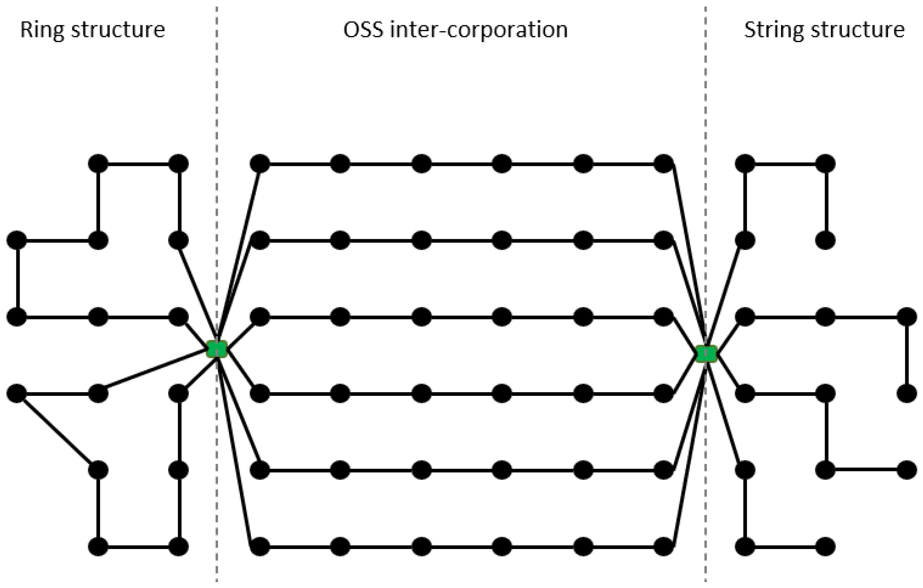
4.7. Incorporation of Multiple OWFs

During the review process, several studies have been found that focus on the optimal incorporation of multiple OWFs and the development of a common export system ([28,83,84,85]). These have not been assessed here, as it would have been out of scope of this study. However, the integration of several wind farms can show great potential for the optimization of the export system, especially when individual wind farm developers are not responsible for transmission to the main grid. Such a separate optimization, however, poses the risk that optimization of the array grid loses the global perspective on the overall problem and thus misses potential savings.
Another aspect that is not considered, since it is not directly related to the individual OWF layout, is the impact of wakes from neighboring wind farms as is currently assessed in the North Sea where bottom-fixed wind farms are planned to be densely populated [86]. Under certain wind conditions, an energy production deficit of up to 20% is reported. Once floating wind will reach a commercial scale, this effect might be valuable to consider regarding the FOWF layout and cabling optimization.
The scheme in Figure 15 wraps up the overall findings and clarifies the key points which will need to find consideration to reach meaningful floating wind-specific grid layout optimizations.

5. Conclusions

This review aimed to identify current state-of-the-art optimization techniques applied to cable routing problems for FOWFs. The literature review has shown that the great majority of research is still very concentrated on the bottom-fixed industry. Only in recent years has research focusing on FOWFs been published occasionally, highlighting some of the new challenges that arise with this nascent technology.
In order to find an optimal cost-effective solution for the inter-array cabling of OWFs, it is necessary to take the whole picture into account, i.e., micrositing, wake effects, cable type selection, long-term effects such as cable power losses, reliability-based availability, etc. This is best carried out using a nested or even simultaneous optimization considering all relevant aspects simultaneously in the optimization process.
Concerning the optimization techniques, deterministic methods do not seem to be able to cope with the increasing sizes of wind farms and the growing complexity of problems in a reasonable computational time. This will be especially the case when looking at the additional complexity which is introduced by considering large-scale FOWFs. Already today in the bottom-fixed-based optimization literature, most papers approach the cabling problem by using metaheuristic methods. The most common are the population-based metaheuristics genetic algorithm and particle swarm optimization. It seems that the PSO, in contrary to the GA, comes with less programming effort and can benefit from the cooperative behavior of particles, whereas the GA promotes the survival of the fittest while leaving poorer solutions to themselves as a product of random mutation and crossover. Besides PSO and GA, some other metaheuristics seem to be able to cope with this complex problem. The variable neighborhood search, tabu search, and the bat algorithm were only encountered in a handful of studies, but seem to produce good results, and it may be worth taking a closer look at them in the future. However, it should be noted that (meta-)heuristics, in general, do not guarantee finding an optimal solution. Therefore, researchers underline the benefits of including a local search phase in the metaheuristics in order to prevent it from falling into a local optimum. On the other hand, the literature has also shown that fully sophisticated metaheuristics are not necessarily needed in order to find good solutions. Clustering heuristics can also provide good solutions or give high-quality initial solutions for metaheuristics in order to ease the searching process.
For future works, treating the cabling optimization of commercial-sized FOWFs, new restrictions and constraints will need to be considered which will make the problem more complex and possibly more time-consuming. In order to find feasible and practical solutions, cabling configurations, station-keeping systems, seabed characteristics, water depths, power losses in the form of wake and cable losses, floating wind-specific control mechanisms, OSS positioning, and reliability and maintainability aspects, amongst others, will need to be taken into consideration by future optimization works to substantially lower the LCOE of commercial-scale FOWFs.

Author Contributions

Conceptualization, M.D.K.; methodology, M.D.K.; writing—original draft preparation, M.D.K.; review and editing, M.D.K., J.I.R., P.T.C. and J.L.D.-G.; All authors have read and agreed to the published version of the manuscript.

Funding

This research was funded by INVESTIGO Programme from the Spanish ministry and by the European Union’s H2020 Programme under Grant Agreement no 815083—COREWIND.

Institutional Review Board Statement

Not applicable.

Data Availability Statement

Not applicable.

Acknowledgments

The authors would like to express their sincere gratitude to Sina Elaine Montag from IREC for her read-through and helpful suggestions for this paper.

Conflicts of Interest

The authors declare no conflict of interest.

Abbreviations

The following abbreviations are used in this manuscript:
AEPAnnual Energy Production
ACAlternating Current
ACOAnt Colony optimization
BABat Algorithm
CAPEXCAPital EXpenditure
DCDirect Current
DECEXDECommissioning EXpenditure
EENSExpected Energy Not Supplied
FCMFuzzy C-Means (clustering)
FOWFFloating Offshore Wind Farm
FOWTFloating Offshore Wind Turbine
GAGenetic Algorithm
HOPHang-Off Point
HVHigh Voltage
IAInter Array (cabling)
LCOELevelized Cost Of Energy
MTTRMean Time To Repair
MSTMinimum Spanning Tree
OPEXOPerational EXpenditures
OSSOffshore Substation
OTMOffshore Transformer Module
OWFOffshore Wind Farm
PCCPoint of Common Coupling
PSOParticle Swarm Optimization
SASimulated Annealing
TDPTouchDown Point
TLPTension-Leg Platform
TSTabu Search
VNSVariable Neighborhood Search
WTWind Turbine

References

  1. Lee, J.; Zhao, F.; Dutton, A.; Backwell, B.; Qiao, L.; Liang, W.; Clarke, E.; Lathigara, A.; Shardul, M.; Smith, M.; et al. Global Offshore Wind Report 2021; Technical Report; GWEC. 2021. Available online: https://gwec.net/global-offshore-wind-report-2021/ (accessed on 20 June 2023).
  2. Pérez-Rúa, J.A.; Cutululis, N.A. A framework for simultaneous design of wind turbines and cable layout in offshore wind. Wind Energy Sci. 2022, 7, 925–942. [Google Scholar] [CrossRef]
  3. Serrano González, J.; Burgos Payán, M.; Santos, J.M.R.; González-Longatt, F. A review and recent developments in the optimal wind-turbine micro-siting problem. Renew. Sustain. Energy Rev. 2014, 30, 133–144. [Google Scholar] [CrossRef]
  4. Ikhennicheu, M.; Lynch, M.; Doole, S.; Borisade, F.; Wendt, F.; Schwarzkopf, M.A.; Matha, D.; Vicente, R.D.; Habekost, T.; Ramirez, L.; et al. D3.1 Review of the state of the art of dynamic cable system design. COREWIND. European Commission. 2020. Available online: https://corewind.eu/wp-content/uploads/files/publications/COREWIND-D3.1-Review-of-the-state-of-the-art-of-dynamic-cable-system-design.pdf (accessed on 20 June 2023).
  5. Pérez-Rúa, J.A.; Cutululis, N. Electrical Cable Optimization in Offshore Wind Farms—A review. IEEE Access 2019, 7, 85796–85811. [Google Scholar] [CrossRef]
  6. Hou, P.; Zhu, J.; Ma, K.; Yang, G.; Hu, W.; Chen, Z. A review of offshore wind farm layout optimization and electrical system design methods. J. Mod. Power Syst. Clean Energy 2019, 7, 975–986. [Google Scholar] [CrossRef]
  7. Lumbreras, S.; Ramos, A. Offshore wind farm electrical design: A review. Wind Energy 2013, 16, 459–473. [Google Scholar] [CrossRef]
  8. Siemens Energy. New AC Grid Access Solution from Siemens: Lighter, Faster, Cheaper. 2015. Available online: https://press.siemens-energy.com/global/en/pressrelease/new-ac-grid-access-solution-siemens-lighter-faster-cheaper (accessed on 20 June 2023).
  9. Cazzaro, D.; Pisinger, D. Balanced cable routing for offshore wind farms with obstacles. Networks 2022, 80, 386–406. [Google Scholar] [CrossRef]
  10. Sun, R.; Abeynayake, G.; Liang, J.; Wang, K. Reliability and Economic Evaluation of Offshore Wind Power DC Collection Systems. Energies 2021, 14, 2922. [Google Scholar] [CrossRef]
  11. Ferguson, A.; de Villiers, P.; Fitzgerald, B.; Matthiesen, J. Benefits in moving the intra-array voltage from 33 kV to 66 kV AC for large offshore wind farms. Carbon Trust 2012, 2012, 1–7. [Google Scholar]
  12. Young, D. Predicting Dynamic Subsea Cable Failure for Floating Offshore Wind; Technical Report; ORE Catapult. 2018. Available online: https://ore.catapult.org.uk/wp-content/uploads/2018/09/Predicting-Dynamic-Subsea-Cable-Failure-for-Floating-Wind-David-Young-AP-0016.pdf (accessed on 20 June 2023).
  13. Wei, S.; Zhang, L.; Xu, Y.; Fu, Y.; Li, F. Hierarchical Optimization for the Double-Sided Ring Structure of the Collector System Planning of Large Offshore Wind Farms. IEEE Trans. Sustain. Energy 2017, 8, 1029–1039. [Google Scholar] [CrossRef]
  14. Zuo, T.; Zhang, Y.; Meng, K.; Tong, Z.; Dong, Z.Y.; Fu, Y. A Two-Layer Hybrid Optimization Approach for Large-Scale Offshore Wind Farm Collector System Planning. IEEE Trans. Ind. Inform. 2021, 17, 7433–7444. [Google Scholar] [CrossRef]
  15. Dahmani, O.; Bourguet, S.; Machmoum, M.; Guerin, P.; Rhein, P.; Josse, L. Optimization and Reliability Evaluation of an Offshore Wind Farm Architecture. IEEE Trans. Sustain. Energy 2017, 8, 542–550. [Google Scholar] [CrossRef]
  16. Ho, W.C. GA based algorithms for offshore wind farm collector cable optimization. J. Phys. Conf. Ser. 2022, 2362, 012017. [Google Scholar] [CrossRef]
  17. Shin, J.S.; Kim, J.O. Optimal Design for Offshore Wind Farm considering Inner Grid Layout and Offshore Substation Location. IEEE Trans. Power Syst. 2017, 32, 2041–2048. [Google Scholar] [CrossRef]
  18. Pillai, A.; Chick, J.; Johanning, L.; Khorasanchi, M. Offshore wind farm layout optimization using particle swarm optimization. J. Ocean Eng. Mar. Energy 2018, 4, 73–88. [Google Scholar] [CrossRef]
  19. Wu, Y.W.; Wang, Y. Collection line optimization in wind farms using improved ant colony optimization. Wind Eng. 2020, 45, 589–600. [Google Scholar] [CrossRef]
  20. Yi, X.; Scutariu, M.; Smith, K. Optimization of offshore wind farm inter-array collection system. IET Renew. Power Gener. 2019, 13, 1990–1999. [Google Scholar] [CrossRef]
  21. Shen, X.; Li, S.; Li, H. Large-scale Offshore Wind Farm Electrical Collector System Planning: A Mixed-Integer Linear Programming Approach, 2021. arXiv 2021, arXiv:2108.08569. [Google Scholar]
  22. Zuo, T.; Zhang, Y.; Meng, K.; Tong, Z.; Dong, Z.Y.; Fu, Y. Collector System Topology Design for Offshore Wind Farm’s Repowering and Expansion. IEEE Trans. Sustain. Energy 2021, 12, 847–859. [Google Scholar] [CrossRef]
  23. Zuo, T.; Zhang, Y.; Meng, K.; Dong, Z.Y. Collector System Topology for Large-Scale Offshore Wind Farms Considering Cross-Substation Incorporation. IEEE Trans. Sustain. Energy 2020, 11, 1601–1611. [Google Scholar] [CrossRef]
  24. Zuo, T.; Meng, K.; Tong, Z.; Tang, Y.; Dong, Z.H. Offshore wind farm collector system layout optimization based on self-tracking minimum spanning tree. Int. Trans. Electr. Energy Syst. 2019, 29, e2729. [Google Scholar] [CrossRef]
  25. Dutta, S.; Overbye, T. A clustering based wind farm collector system cable layout design. In Proceedings of the 2011 IEEE Power and Energy Conference, Urbana, IL, USA, 25–26 February 2011. [Google Scholar] [CrossRef]
  26. Dutta, S.; Overbye, T.J. Optimal Wind Farm Collector System Topology Design Considering Total Trenching Length. IEEE Trans. Sustain. Energy 2012, 3, 339–348. [Google Scholar] [CrossRef]
  27. Cazzaro, D.; Fischetti, M.; Fischetti, M. Heuristic algorithms for the Wind Farm Cable Routing problem. Appl. Energy 2020, 278, 115617. [Google Scholar] [CrossRef]
  28. Hardy, S.; Ergun, H.; Van Hertem, D. Application of Association Rule Mining in offshore HVAC transmission topology optimization. Electr. Power Syst. Res. 2022, 211, 108358. [Google Scholar] [CrossRef]
  29. Pérez-Rúa, J.A.; Stolpe, M.; Das, K.; Cutululis, N. Global Optimization of Offshore Wind Farm Collection Systems. IEEE Trans. Power Syst. 2020, 35, 2256–2267. [Google Scholar] [CrossRef]
  30. Pérez-Rúa, J.A.; Lumbreras, S.; Ramos, A.; Cutululis, N.A. Reliability-based topology optimization for offshore wind farm collection system. Wind Energy 2022, 25, 52–70. [Google Scholar] [CrossRef]
  31. Cerveira, A.; Pires, E.J.S.; Baptista, J. Wind Farm Cable Connection Layout Optimization with Several Substations. Energies 2021, 14, 3615. [Google Scholar] [CrossRef]
  32. Pérez-Rúa, J.A.; Stolpe, M.; Cutululis, N.A. Integrated Global Optimization Model for Electrical Cables in Offshore Wind Farms. IEEE Trans. Sustain. Energy 2020, 11, 1965–1974. [Google Scholar] [CrossRef]
  33. Klein, A.; Haugland, D. Obstacle-aware optimization of offshore wind farm cable layouts. Ann. Oper. Res. 2019, 272, 373–388. [Google Scholar] [CrossRef]
  34. Ulku, I.; Alabas-Uslu, C. Optimization of cable layout designs for large offshore wind farms. Int. J. Energy Res. 2020, 44, 6297–6312. [Google Scholar] [CrossRef]
  35. Marge, T.; Lumbreras, S.; Ramos, A.; Hobbs, B.F. Integrated offshore wind farm design: Optimizing micro-siting and cable layout simultaneously. Wind Energy 2019, 22, 1684–1698. [Google Scholar] [CrossRef]
  36. Ulku, I.; Uslu, C. Optimization of offshore wind farm cable layouts. In Proceedings of the The Sixth European Conference on Renewable Energy Systems, Istanbul, Turkey, 25–27 June 2018. [Google Scholar]
  37. Pérez-Rúa, J.A.; Lumbreras, S.; Ramos, A.; Cutululis, N. Closed-Loop Two-Stage Stochastic Optimization of Offshore Wind Farm Collection System. J. Phys. Conf. Ser. 2020, 1618, 042031. [Google Scholar] [CrossRef]
  38. Lumbreras, S.; Ramos, A. Optimal design of the electrical layout of an offshore wind farm applying decomposition strategies. IEEE Trans. Power Syst. 2013, 28, 1434–1441. [Google Scholar] [CrossRef]
  39. Serrano González, J.; Trigo García, A.L.; Burgos Payán, M.; Riquelme Santos, J.; González Rodríguez, A.G. Optimal wind-turbine micro-siting of offshore wind farms: A grid-like layout approach. Appl. Energy 2017, 200, 28–38. [Google Scholar] [CrossRef]
  40. Gong, X.; Kuenzel, S.; Pal, B. Optimal Wind Farm Cabling. IEEE Trans. Sustain. Energy 2017, 9, 1126–1136. [Google Scholar] [CrossRef]
  41. Kershenbaum, A. Computing capacitated minimal spanning trees efficiently. Networks 1974, 4, 299–310. [Google Scholar] [CrossRef]
  42. Holland, J.H. Genetic Algorithms. Sci. Am. 1992, 267, 66–73. [Google Scholar] [CrossRef]
  43. Wang, L.; Wu, J.; Tang, Z.; Wang, T. An Integration Optimization Method for Power Collection Systems of Offshore Wind Farms. Energies 2019, 12, 3965. [Google Scholar] [CrossRef]
  44. Wade, B.; Pereira, R.; Wade, C. Investigation of offshore wind farm layouts regarding wake effects and cable topology. J. Phys. Conf. Ser. 2019, 1222, 012007. [Google Scholar] [CrossRef]
  45. Wei, S.; Feng, Y.; Liu, K.; Fu, Y. Optimization of Power Collector System for Large-scale Offshore Wind Farm Based on Topological Redundancy Assessment. E3S Web Conf. 2020, 194, 03025. [Google Scholar] [CrossRef]
  46. Wu, Y.; Zhang, S.; Wang, R.; Wang, Y.; Feng, X. A design methodology for wind farm layout considering cable routing and economic benefit based on genetic algorithm and GeoSteiner. Renew. Energy 2020, 146, 687–698. [Google Scholar] [CrossRef]
  47. Bauer, J.; Lysgaard, J. The offshore wind farm array cable layout problem: A planar open vehicle routing problem. J. Oper. Res. Soc. 2015, 66, 360–368. [Google Scholar] [CrossRef]
  48. Juhl, D.; Warme, D.M.; Winter, P.; Zachariasen, M. The GeoSteiner software package for computing Steiner trees in the plane: An updated computational study. Math. Program. Comput. 2018, 10, 487–532. [Google Scholar] [CrossRef]
  49. Roetert, T.; Raaijmakers, T.; Borsje, B. Cable route optimization for offshore wind farms in morphodynamic areas. In Proceedings of the 27th International Ocean and Polar Engineering Conference, ISOPE 2017, San Francisco, CA, USA, 25–30 June 2017; Society of Petroleum Engineers: Richardson, TX, USA, 2017; pp. 595–606. [Google Scholar]
  50. Lerch, M.; De-Prada-Gil, M.; Molins, C. A metaheuristic optimization model for the inter-array layout planning of floating offshore wind farms. Int. J. Electr. Power Energy Syst. 2021, 131, 107128. [Google Scholar] [CrossRef]
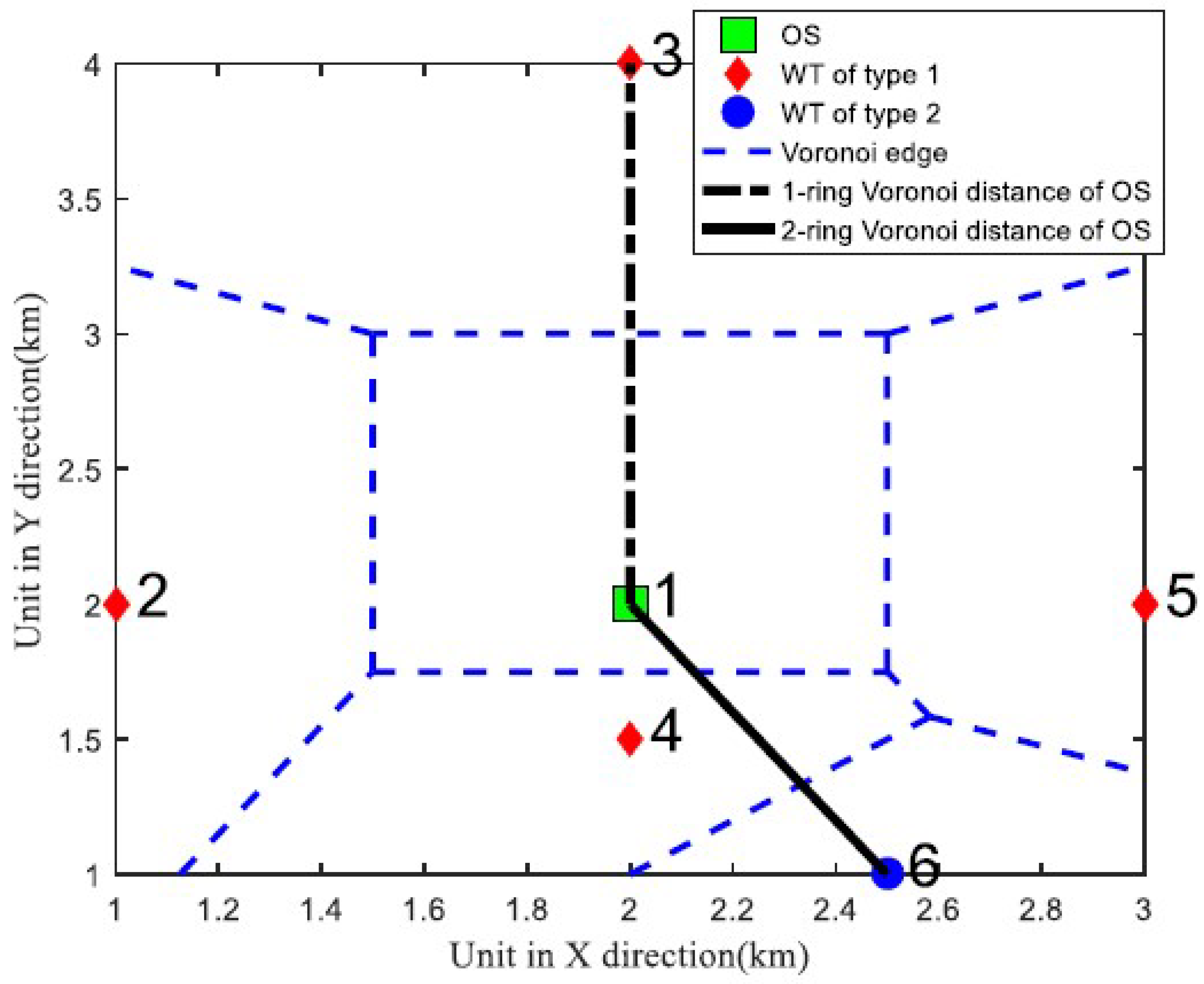
  51. Qi, Y.; Hou, P.; Liu, G.; Jin, R.; Yang, Z.; Yang, G.; Dong, Z. Cable Connection Optimization for Heterogeneous Offshore Wind Farms via a Voronoi Diagram Based Adaptive Particle Swarm Optimization with Local Search. Energies 2021, 14, 644. [Google Scholar] [CrossRef]
  52. Tao, S.; Xu, Q.; Feijóo, A.; Zheng, G. Joint Optimization of Wind Turbine Micrositing and Cabling in an Offshore Wind Farm. IEEE Trans. Smart Grid 2021, 12, 834–844. [Google Scholar] [CrossRef]
  53. El Mokhi, C.; Addaim, A. Optimization of Wind Turbine Interconnections in an Offshore Wind Farm Using Metaheuristic Algorithms. Sustainability 2020, 12, 5761. [Google Scholar] [CrossRef]
  54. Jin, R.; Hou, P.; Yang, G.; Qi, Y.; Chen, C.; Chen, Z. Cable routing optimization for offshore wind power plants via wind scenarios considering power loss cost model. Appl. Energy 2019, 254, 113719. [Google Scholar] [CrossRef]
  55. Hou, P.; Yang, G.; Hu, W.; Chen, C.; Soltani, M.; Chen, Z. Cable Connection Scheme Optimization for Offshore Wind Farm Considering Wake Effect. In Proceedings of the 2018 IEEE Congress on Evolutionary Computation (CEC), Rio de Janeiro, Brazil, 8–13 July 2018; pp. 1–8. [Google Scholar] [CrossRef]
  56. Hou, P.; Hu, W.; Soltani, M.; Chen, C.; Chen, Z. Combined optimization for offshore wind turbine micro siting. Appl. Energy 2017, 189, 271–282. [Google Scholar] [CrossRef]
  57. Pillai, A.; Chick, J.; Johanning, L.; Khorasanchi, M.; de Laleu, V. Offshore wind farm electrical cable layout optimization. Eng. Optim. 2015, 47, 1689–1708. [Google Scholar] [CrossRef]
  58. Hou, P.; Hu, W.; Chen, Z. Optimization for offshore wind farm cable connection layout using adaptive particle swarm optimization minimum spanning tree method. IET Renew. Power Gener. 2016, 10, 694–702. [Google Scholar] [CrossRef]
  59. Pookpunt, S.; Ongsakul, W. Optimal placement of wind turbines within wind farm using binary particle swarm optimization with time-varying acceleration coefficients. Renew. Energy 2013, 55, 266–276. [Google Scholar] [CrossRef]
  60. Taylor, P.; Yue, H.; Campos-Gaona, D.; Anaya-Lara, O.; Jia, C. Wind farm array cable layout optimization for complex offshore sites - a decomposition based heuristic approach. IET Renew. Power Gener. 2023, 17, 243–259. [Google Scholar] [CrossRef]
  61. Fischetti, M.; Pisinger, D. Optimizing wind farm cable routing considering power losses. Eur. J. Oper. Res. 2018, 270, 917–930. [Google Scholar] [CrossRef]
  62. Fischetti, M.; Pisinger, D. Optimal wind farm cable routing: Modeling branches and offshore transformer modules. Networks 2018, 72, 42–59. [Google Scholar] [CrossRef]
  63. Yang, X.S. A New Metaheuristic Bat-Inspired Algorithm. In Nature Inspired Cooperative Strategies for Optimization (NICSO 2010); Springer: Berlin/Heidelberg, Germany, 2010; pp. 65–74. [Google Scholar] [CrossRef]
  64. Qi, Y.; Hou, P.; Yang, L.; Yang, G. Simultaneous Optimization of Cable Connection Schemes and Capacity for Offshore Wind Farms via a Modified Bat Algorithm. Appl. Sci. 2019, 9, 265. [Google Scholar] [CrossRef]
  65. Srinivas, M.; Patnaik, L. Adaptive probabilities of crossover and mutation in genetic algorithms. IEEE Trans. Syst. Man Cybern. 1994, 24, 656–667. [Google Scholar] [CrossRef]
  66. Pillai, A.C.; Chick, J.; Khorasanchi, M.; Barbouchi, S.; Johanning, L. Application of an offshore wind farm layout optimization methodology at Middelgrunden wind farm. Ocean Eng. 2017, 139, 287–297. [Google Scholar] [CrossRef]
  67. Hassan, R.; Cohanim, B.; de Weck, O.; Venter, G. A Comparison of Particle Swarm Optimization and the Genetic Algorithm. In Proceedings of the 46th AIAA/ASME/ASCE/AHS/ASC Structures, Structural Dynamics and Materials Conference, Austin, TX, USA, 18–21 April 2005. [Google Scholar] [CrossRef]
  68. Eberhart, R.; Kennedy, J. A new optimizer using particle swarm theory. In Proceedings of the MHS’95 Sixth International Symposium on Micro Machine and Human Science, Nagoya, Japan, 4–6 October 1995; pp. 39–43. [Google Scholar] [CrossRef]
  69. Rapha, J.I.; Domínguez, J.L. Suspended cable model for layout optimization purposes in floating offshore wind farms. J. Phys. Conf. Ser. 2021, 2018, 012033. [Google Scholar] [CrossRef]
  70. Ahmad, I.B.; Schnepf, A.; Ong, M.C. An optimization methodology for suspended inter-array power cable configurations between two floating offshore wind turbines. Ocean Eng. 2023, 278, 114406. [Google Scholar] [CrossRef]
  71. Lerch, M.; De-Prada-Gil, M.; Molins, C. Collection Grid Optimization of a Floating Offshore Wind Farm Using Particle Swarm Theory. J. Phys. Conf. Ser. 2019, 1356, 012012. [Google Scholar] [CrossRef]
  72. Banzo, M.; Ramos, A. Stochastic Optimization Model for Electric Power System Planning of Offshore Wind Farms. IEEE Trans. Power Syst. 2011, 26, 1338–1348. [Google Scholar] [CrossRef]
  73. Rodrigues, S.; Teixeira Pinto, R.; Soleimanzadeh, M.; Bosman, P.A.; Bauer, P. Wake losses optimization of offshore wind farms with moveable floating wind turbines. Energy Convers. Manag. 2015, 89, 933–941. [Google Scholar] [CrossRef]
  74. Annoni, J.; Seiler, P.; Johnson, K.; Fleming, P.; Gebraad, P. Evaluating wake models for wind farm control. In Proceedings of the 2014 American Control Conference, Portland, OR, USA, 4–6 June 2014. [Google Scholar] [CrossRef]
  75. Kheirabadi, A.C.; Nagamune, R. Real-time relocation of floating offshore wind turbine platforms for wind farm efficiency maximization: An assessment of feasibility and steady-state potential. Ocean Eng. 2020, 208, 107445. [Google Scholar] [CrossRef]
  76. Serrano González, J.; Burgos Payán, M.; Riquelme Santos, J.M.; González Rodríguez, A.G. Optimal Micro-Siting of Weathervaning Floating Wind Turbines. Energies 2021, 14, 886. [Google Scholar] [CrossRef]
  77. Mahfouz, M.Y.; Cheng, P.W. A passively self-adjusting floating wind farm layout to increase the annual energy production. Wind Energy 2023, 26, 251–265. [Google Scholar] [CrossRef]
  78. Nanos, E.M.; Bottasso, C.L.; Tamaro, S.; Manolas, D.I.; Riziotis, V.A. Vertical wake deflection for floating wind turbines by differential ballast control. Wind Energy Sci. 2022, 7, 1641–1660. [Google Scholar] [CrossRef]
  79. Ramos-García, N.; Kontos, S.; Pegalajar-Jurado, A.; Horcas, S.G.; Bredmose, H. Investigation of the floating IEA Wind 15 MW RWT using vortex methods Part I: Flow regimes and wake recovery. Wind Energy 2022, 25, 468–504. [Google Scholar] [CrossRef]
  80. Bills, G. Offshore Wind’s Reactive Power. 2022. Available online: https://www.infrastructureinvestor.com/offshore-winds-reactive-power/ (accessed on 20 June 2023).
  81. Schwarzkopf, M.A.; Borisade, F.; Matha, D.; Kallinger, M.D.; Mahfouz, M.Y.; Duran Vicente, R.; Munoz, S. D4.1 Identification of floating-wind-specific O&M requirements and monitoring technologies. COREWIND. European Commission. 2020. Available online: https://corewind.eu/wp-content/uploads/files/publications/COREWIND-D4.1-Identification-of-floating-wind-specific-O-and-M-requirements-and-monitoring-technologies.pdf (accessed on 20 June 2023).
  82. Avanessova, N.; Gray, A.; Lazakis, I.; Thomson, R.C.; Rinaldi, G. Analysing the effectiveness of different offshore maintenance base options for floating wind farms. Wind Energy Sci. 2022, 7, 887–901. [Google Scholar] [CrossRef]
  83. Hardy, S.; Van Brusselen, K.; Van Hertem, D.; Ergun, H. A Techno-Economic MILP Optimization of Multiple Offshore Wind Concessions. In Proceedings of the Wind Energy Science Conference 2019 (WESC 2019), Cork, Ireland, 17–20 June 2020. [Google Scholar]
  84. Hardy, S.; Ergun, H.; Van Hertem, D. A Greedy Algorithm for Optimizing Offshore Wind Transmission Topologies. IEEE Trans. Power Syst. 2022, 37, 2113–2121. [Google Scholar] [CrossRef]
  85. Liu, Y.; Fu, Y.; Huang, L.L.; Ren, Z.X.; Jia, F. Optimization of offshore grid planning considering onshore network expansions. Renew. Energy 2022, 181, 91–104. [Google Scholar] [CrossRef]
  86. Baas, P.; Verzijlbergh, R. The Impact of Wakes from Neighboring Wind Farms on the Production of the IJmuiden Ver Wind Farm Zone; Technical Report; Whiffle and TU Delft: Delft, The Netherlands, 2022; Available online: https://whiffle.nl/wp-content/uploads/2022/12/The-impact-of-wakes-from-neighboring-wind-farms-IJmuiden.pdf (accessed on 20 June 2023).
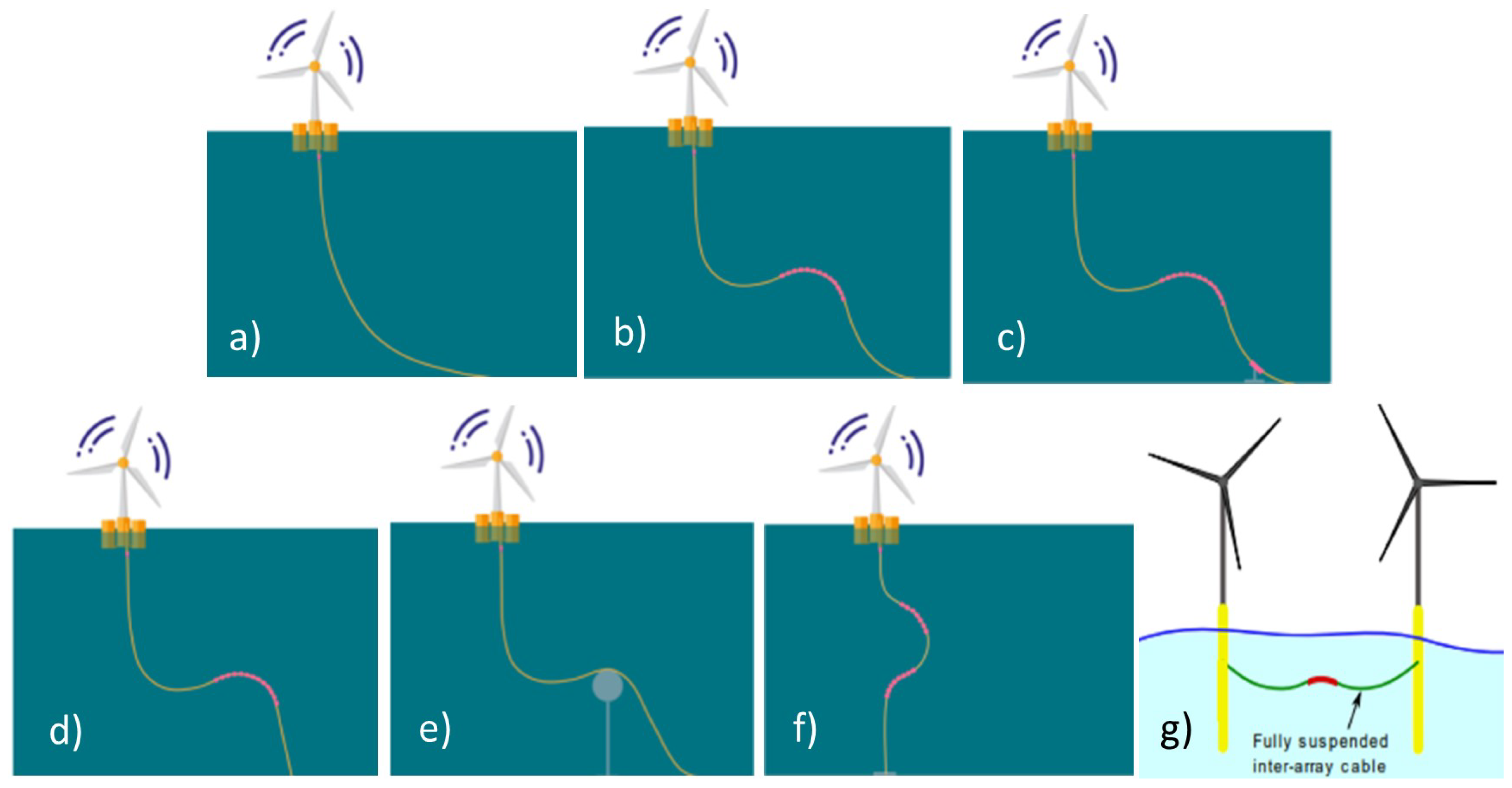
Figure 1. Comparison of the amount of studied literature published since 2019.
Cleantechnol 05 00039 g001
Figure 2. Number of turbines to be supported by a cable in a string (left) and ring (right) structure.
Cleantechnol 05 00039 g002
Figure 3. OSS positioning approaches used in the analyzed literature since 2019.
Cleantechnol 05 00039 g003
Figure 4. OSS location refinement based on export cabling.
Cleantechnol 05 00039 g004
Figure 5. Optimization methodologies in the analyzed literature published since 2019.
Cleantechnol 05 00039 g005
Figure 6. (ac): Examples of Steiner nodes (blue) used for laying a cable around a turbine (black).
Cleantechnol 05 00039 g006
Figure 7. OSS inter-corportaion.
Cleantechnol 05 00039 g007
Figure 8. Multi-loop structure.
Cleantechnol 05 00039 g008
Figure 9. Metaheuristics used in the analyzed literature since 2019.
Cleantechnol 05 00039 g009
Figure 10. (a) Minimum spanning tree; (b) Euclidean minimum Steiner tree.
Cleantechnol 05 00039 g010
Figure 11. Shortest paths from WTs to OSS computed using a visibility graph for exclusion zone avoidance ([9]).
Cleantechnol 05 00039 g011
Figure 12. K-shaped Voronoi diagram ([51]).
Cleantechnol 05 00039 g012
Figure 13. Different configurations of dynamic cables: (a) free hanging (catenary), (b) lazy wave, (c) tethered wave (reverse pliant wave), (d) steep wave, (e) lazy S, (f) Chinese lantern (all [4]) and (g) W-shaped (adapted from [69]).
Cleantechnol 05 00039 g013
Figure 14. Weathervaning FOWT ([76]).
Cleantechnol 05 00039 g014
Figure 15. Key take-aways for meaningful floating wind specific electrical grid optimizations.
Cleantechnol 05 00039 g015
Table 1. Advantages and drawbacks of common dynamic cable configuration (adapted from [4]).
TypeDescriptionAdvantagesDisadvantages
(a) CatenaryFree hanging to seabed
-
Simplest configuration
-
Lowest cost solution
-
Floater motion not decoupled
-
No restriction of lateral motion
-
High tension at HOP *
-
Bend stiffener at HOP required
-
Unsuitable for significant dynamic motions and great water depths
(b) Lazy
wave
Attached buoyancy modules provide lift at midwater cable section
-
Simple configuration
-
Decoupling of floater motions from TDP **
-
Proven use for deep water application
-
Low cost solution
-
No restriction of lateral motion
-
Prone to marine growth depending on depth
-
Bend stiffener at HOP required
-
Buoyancy modules required
-
Critical where distance between HOP and TDP is restricted
-
Strong currents may lead to TDP migration
(c) Tethered
wave
Similar to lazy wave with additional tether restraining TDP
-
Decoupling of floater motions from TDP
-
Reduced freedom of TDP under cross current
-
Higher levels of marine growth possible due to tethered TDP
-
Mid-range cost solution
-
Tether and clamp complicate installation
-
Prone to marine growth depending on depth
-
Bend stiffener at HOP required
-
Buoyancy modules required
(d) Steep
wave
Similar to lazy wave but connection to seabed junction is made vertically via bend stiffener
-
Decoupling of floater motions from TDP
-
Limited changes in configuration with higher levels of marine growth
-
Subsea base reduces excursion under current
-
Reduced distance between HOP and TDP
-
Bend stiffeners at HOP and TDP required
-
Buoyancy modules required
-
High cost solution given additional termination units
(e) Lazy SSimilar to lazy wave but with subsea buoy (fixed or floating) creating mid-water arch
-
Decoupling of floater motions from TDP
-
Limited changes in configuration due to marine growth
-
Subsea buoy reducing excursion under cross current
-
Sag bend (arch open to the top) carefully controlled (good for offset control)
-
Suitable for multiple cables approaching hub (e.g., OSS)
-
Bend stiffener at HOP required
-
Buoyant mid-water arch, clamps and maybe tether required
-
Fixed sag bend location
-
High-cost solution; may not be economical for a single cable
-
Minimum separation distance on buoy may become critical (danger of cable clashing and current rating reduction)
(f) Chinese
lantern
U-shaped slacked keeping tether vertically aligned with HOP
-
Decoupling of floater motions from TDP
-
Subsea base reduces excursions under cross currents and prevents migration of TDP
-
Reduced distance between HOP and TDP
-
Accommodates significant upward motions (heave)
-
Bend stiffener at HOP and TDP required
-
Buoyancy modules required
-
Limited regarding water depth
-
Unsuitable for dynamic motions with large offsets
(g) w-shapedSuspended between floaters without touching seabed and aided by buoyancy modules
-
Short cable length for great water depths
-
Avoidance of TDP and trenching
-
Low-cost solution
-
Buoyancy modules required
-
Bend stiffener at HOPs required
-
Prone to marine growth and cross currents
-
Motions of connected floaters need to be accurately assessed
-
Feasibility not fully proven
* HOP = Hang-off point; ** TDP = Touchdown point
Disclaimer/Publisher’s Note: The statements, opinions and data contained in all publications are solely those of the individual author(s) and contributor(s) and not of MDPI and/or the editor(s). MDPI and/or the editor(s) disclaim responsibility for any injury to people or property resulting from any ideas, methods, instructions or products referred to in the content.

