Article

Soil Erosion Spatial Prediction using Digital Soil Mapping and RUSLE methods for Big Sioux River Watershed

by
Ruhollah Taghizadeh-Mehrjardi
1,2,*,
Arun Bawa
3,
Sandeep Kumar
3,*,
Mojtaba Zeraatpisheh
4,5,
Alireza Amirian-Chakan
6 and
Ali Akbarzadeh
7
1
Department of Geosciences, Soil Science and Geomorphology, University of Tübingen, 72070 Tübingen, Germany
2
Faculty of Agriculture and Natural Resources, Ardakan University, Ardakan 8951656767, Iran
3
Department of Agronomy, Horticulture and Plant Science, South Dakota State University, Brookings, SD 57007, USA
4
Key Laboratory of Geospatial Technology for the Middle and Lower Yellow River Regions, College of Environment and Planning, Henan University, Kaifeng 475004, China
5
Department of Soil Science, Ramin Agriculture and Natural Resources University of Khuzestan, Ahvaz 6341773637, Iran
6
Department of Soil Science, Lorestan University, Khorramabad 6815144316, Iran
7
Department of Soil Science, Faculty of Agriculture, Shahrekord University, Shahrekord 8818634141, Iran
*
Authors to whom correspondence should be addressed.
Soil Syst. 2019, 3(3), 43; https://doi.org/10.3390/soilsystems3030043
Submission received: 16 April 2019 / Revised: 2 July 2019 / Accepted: 4 July 2019 / Published: 8 July 2019
(This article belongs to the Special Issue Soil Erosion and Land Degradation)

Abstract

:
A recent conversion of the grasslands to cropland degrading the soil quality (SQ), and impacting the soil erosion and crop productivity in the West Corn Belt (WCB) of the USA. The current study was conducted to estimate the spatial distribution of soil erosion at Big Sioux River (BSR) watershed scale using the Geographical Information System (GIS)-enabled Revised Universal Soil Loss Equation (RUSLE). Spatial data such as weather, a digital elevation model (DEM), land use maps and soils were used for assessment of soil erosion was downloaded from the easily available online sources. Data showed that about 7% of grassland acreage reduced from 2008 (24%) to 2015 (17%), whereas, about 7.4% of cropland acreage increased from 2008 (64.6%) to 2015 (72%) in the BSR watershed. This grassland conversion to cropland increased the soil erosion (estimated using the RUSLE model) from 12.2 T ha−1 year−1 in 2008 to 14.8 T ha−1 year−1 in 2015. The present study concludes that grassland conversion to cropland in the BSR watershed increased the soil erosion, therefore, management practices essential to be applied to reduce the erosion risk and various other ecosystem services.

1. Introduction

A recent land use change (LUC) in the West Corn Belt (WCB) region of USA poses a threat to grasslands [1] that play a significant role in climate regulation, water and soil conservation, and biodiversity maintenance. Grassland conversion to cropland increases soil erosion and degrades soil quality (SQ). Soil erosion has been identified as one of the biggest challenges to the environment globally [2,3]. It not only degrades soil structure but also increases the loss of organic matter, reduces soil depth and nutrient elements [4,5]. The shift from grasslands to cropland has scaled up due to the increase in the return prices of soybean (Glycine max) and corn (Zea mays), as the demand of biofuel feedstock has been increased in the WCB region of USA [1]. These row crops (corn and soybean), converted from grasslands require intensive soil disturbance which led to the highest amount of soil organic carbon (SOC) and soil losses. Furthermore, an increase in greenhouse gas (GHG) emissions has also been estimated with the LUC for the biofuels, thereby, reducing the biodiversity in the U.S. corn and soybean fields by about 60% [6]. The cropland change consequently affects carbon dynamics [7].
Land use conversion strongly impacts the loss of SOC and influences the global climate change. [8]. Further, this depleted SOC has been exacerbated by the increasing demands for food, biomass and ethanol production, and affects climatic change due to increases in C fluxes, and global warming. In the Midwest region, it is predicted around 6 million metric tons of N fertilizer and over 100,000 metric tons of pesticides are spread over the crop fields [9], which subsequently degrade the SQ and impair the water quality of the streams. Soil erosion in agricultural lands is one of the main reasons of land degradation and water quality decline in the USA [10,11]. Row crops converted from grassland in the WCB region uses conventional tillage practices, such as, moldboard plowing which contributed significantly to erosion [12]. Therefore, an accurate estimation of soil erosion with the change in land use is very important.
Soil erosion from row crops depends on various factors such as surface roughness, rainfall intensity, slope, and soil type [3,13]. Surface roughness which is created by leaving crop residue on the ground reduces the velocity of overland flow and reduces soil loss. It is a hard mission to assess the impacts of various soil factors under different cropping systems and climatic conditions on soil loss and productivity. Therefore, different empirical and mechanistic models were established to predict the soil loss [3]. An empirical model, the Universal Soil Loss Equation (USLE), was developed in 1930s by the National Runoff and Soil Loss Data Center and culminating in Agriculture Handbook 537 [14] to estimate the annual soil loss. In the current study, we have estimated the soil erosion potential using the GIS and RUSLE [15,16].
For predicting the average annual soil loss using RUSLE method, six grid-based maps (i.e., rainfall erosivity, soil erodibility, length-slope, vegetation cover, and soil conservation practices) are simply multiplied [14]. Of six factors, the concept of soil erodibility (K factor) and how to predict such a complex parameter has always been a challenging issue [3,17,18,19,20]. There are several types of conventional methods to measure/predict K factor including measurement by scouring, measuring soil physiochemical properties, plot experiment and rainfall simulation, [21] but most of them are time-consuming, expensive, and labor work [22]. Furthermore, in the previous researches K factor commonly calculated from soil properties such as soil texture, soil organic matter, soil structure, and soil permeability class [18], by plot data [14], or by using chroplet maps. Since the knowledge of the spatial patterns of K factor is vital, digital soil mapping (DSM) techniques based on the scorpan model [23] are promising approaches to overcome some limitations arising from the chroplet maps. This technique has progressed rapidly in the field of soil science and precision agriculture in the past decade [24] and has been successfully applied to predict different soil properties and soil classes [25,26]. To best of our knowledge, less research has been carried out to examine the potential of DSM for the spatial prediction of K factor [3], with the notable exception of Yang et al. [27].
The present study based on the hypothesis that conversion of grassland to cropland can degrade the soil structure and can increase the soil erosion. Consequently, the current study was carried out to estimate the soil erosion at a watershed scale which is located within the WCB region. The specific goal of the study was to predict the spatial distribution of soil erosion after the conversion of grassland to cropland at the watershed using the GIS-enabled RUSLE technique. Importantly, in the current study K factor was digitally predicted for the whole study area using digital soil mapping (DSM) techniques. To achieve the goal, we firstly trained an artificial neural network (ANN) using the point-based K factor data and grid-based ancillary data (i.e., terrain attributes and remote sensing data). Then, the trained ANN model was implemented to predict K factor for the whole study area.

2. Materials and Methods
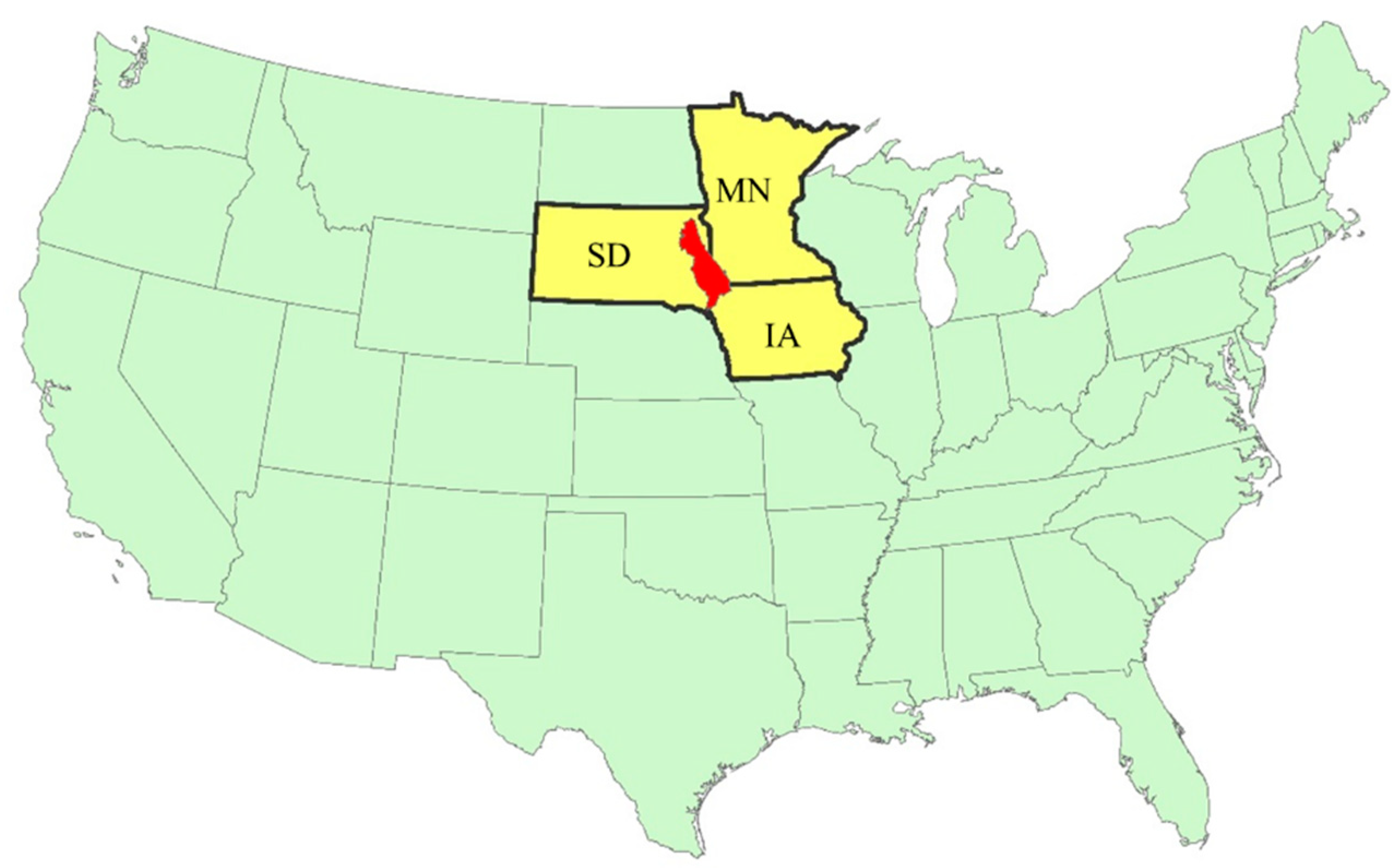
2.1. Study Area

The Big Sioux River (BSR) watershed covering an area of 21,033 km2 is located in the eastern part of South Dakota, the USA (Figure 1). At the study watershed, the mean annual temperature is 7.6 °C that maximum and minimum of temperature occurred in July and January −7.3 and 22.7 °C, respectively. The majority of the BSR watershed has low elevation varies from 334 to 641 m. This relatively flat landscape watershed is primarily dominated by cropland (72%), followed by grassland, urban, water, and wetland. Corn and soybean are major crops of the region, covering around 62% of the total watershed area. Pasture and hay also contribute a significant portion of land use during the growing season. Spring wheat, winter wheat, and oats are the other main crops and cover a small portion (4.5%) of the watershed. Dominant soils are developed on Dakota Sandstone, Granerous Shale, Precambrian Sioux Quartzite, Carlile Shale, Greenhorn Limestone, Pierre Shale and Niobrara Chalk, and consist a heterogeneous mixture of sand, silt, clay, and gravel. Largely covered by loamy glacial till mollisol with low potential-runoff under thoroughly wet conditions, the BSR watershed soils majorly belongs to hydrological soil group ‘B’ having moderate infiltration rates [28].

2.2. RUSLE Model Soil Erosion Calculation

Revised Universal Soil Loss Equation (RUSLE) [16] was used to predict the mean annual soil loss at the BSR watershed. The erosion plot and rainfall simulator experiments by composing of the following factors were used to develop this equation:
A = [ R ] × [ K ] × [ L S ] × [ C ] × [ P ]
where A is the mean soil loss (T ha−1 year−1), R is the rainfall erosivity factor (MJ mm ha−1 h−1 year−1), K is the soil erodibility factor (t h MJ−1 mm−1), LS is the topographic factors (L, slope length and S, slope steepness; dimensionless), C is the vegetation cover (dimensionless), and P is the soil conservation practices (dimensionless). In this study, three long-term scenarios were used for predicting soil erosion that include: 2008, 2010 and 2015 assuming constant rainfall erosivity (R) and estimated R from Regional Climate models [29]. These long-term scenarios will be used for grasslands and row crops separately for 2008, 2010 and 2015 years and the difference in soil erosion will give an estimate of the potential change in erosion that occurred due to grasslands conversion into croplands. Khanal et al. [6] predicted soil loss using the RUSLE with the change in biofuel production for the USA, however, C factor used by these researchers is questionable since the value of C depends on the number of cultivation years. Therefore, at present research, land use change (LUC) from 2008 through 2015 were extracted from National Agricultural Statistics Service (NASS)-Cropland Data Layer (CDL) and C factor values used based on years after the conversion of row crops from grasslands. All the parameters in RUSLE were considered to be spatially constant for every 30-m grid within the digital elevation model (DEM), and mean soil loss (A; T ha−1 year−1) calculated by multiplying all the parameters of Equation (1). Data sources used for soil erosion prediction are explained in the next sections. Land cover data for 2008, 2010 and 2015 were converted to raster format and resampled for 30-m resolution using ArcGIS10x version to create a business as usual (BAU) map. The relative erosion maps were extrapolated for 2008, 2010, 2015 periods.

2.2.1. Rainfall Erosivity Factor (R)

The interaction between the kinetic energy of raindrops and soil surface reflects by the rainfall erosivity factor (R), and it depends on the amount of precipitation in a certain time period [14]. In this study, we have used the monthly rainfall data of 8 years (2008 to 2015) from the 93 rain gauge stations (Figure 2) in and around the study watershed area. Ordinary kriging technique was implemented in order to interpolate the average monthly rainfall [3]. Then, R factor was calculated using the rainfall maps and the modified Fournier index (Equation (2)) and models (Equations (3) and (4)) defined by Renard and Freimund [30]:
F = i = 1 12 p i 2 i = 1 12 p
R = 0.07397 F 1.847 , when F < 55 mm
R = 95.77 6.081 F + 0.4770 F 2 , when F 55 mm
where F is the modified Fournier index, R is the rainfall erosivity factor, Pi is the monthly precipitation (mm), and P is the yearly precipitation (mm).

2.2.2. Soil Erodibility (K)

The value of K depends on the soil properties and is defined by quantifying of soil loss under a standard unit plot condition [3,13,14]. K factor data for 200 soil samples (Figure 2) in the BSR watershed were downloaded from Soil Survey Geographic Data (SSURGO). The summary statistics of the related basic soil information to K factor in the study area is presented in Table 1. We then used artificial neural networks (ANN) to correlate value of K (point data) with ancillary variables (grid data) according to the scorpan framework [23] in order to generate K gridded map across the study area with spatial resolution of 30 × 30 m.
The digital soil mapping (DSM) relies on the scorpan spatial prediction function [23]:
S = f ( s , c , o , r , p , a , n ) + e
where S is a soil property (e.g., Soil erodibility), f is a function (e.g., ANN) and scorpan factors are soil, climate, organisms, relief, parent materials, age and spatial position, respectively; and where e is the error. In the current study, based on the understanding of the factors which may affect soil erodibility distribution and availability of such ancillary data [31], two kinds of ancillary variables listed in Table 1 were used. These ancillary data included terrain attributes and remote sensing data. Specifically, a total of 10 terrain attributes extracted from a preprocessed SRTM DEM (Shuttle Radar Topography Mission Digital Elevation Model) using Saga GIS software [32]. A total of 10 remote sensing indices extracted from Landsat 8 Operational Land Imager (OLI) images. The digital numbers (DN) of each spectral band of OLI were calibrated to satellite radiances and then atmospheric correction was performed using the dark-object subtraction (DOS) technique [33]. Here, we calculated the median values of DN of 1584 remote sensed images obtained from 2008 to 2010 (summer season) which were consistent with the soil sampling date.

2.2.3. Topographic Factor (LS)

Topographic factor (LS) represents a ratio of soil loss for a unit area at a specific site in comparison with that under a standard unit plot condition [3,14,34]. At present research, for watershed scale erosion modelling, a DEM with 30 by 30-m resolution (Figure 2) was applied to estimate LS factor in GIS environment base on the following equation [35]:
L S = ( m + 1 ) ( U L 0 ) m ( s i n β S 0 ) n
where LS is a topographic factor, U (m2 m−1) upslope contributing area per unit width as a proxy for discharge, U = flow accumulation × cell size, L0: length of the unit plot (22.1 m), S0: slope of unit plot (0.09), β slope, m (sheet) and n (rill) depend on the prevailing type of erosion (m = 0.4 to 0.6) and n (1.0 to 1.3). A detail information about LS factor calculation for RUSLE can be found in [3,35].

2.2.4. Crop Management (C)

This factor indicates the effects of plants, soil cover and soil biomass on erosion. C factor represents the ratio of soil loss for a unit area at a specific site in comparison with that under clean-tilled continuous-fallow conditions [3,14,16,34]. To determine C factor values for the watershed scale, land use-land cover maps (Figure 2) of the study area were downloaded and then converted to C factor according to RUSLE guide tables [34]. Furthermore, in the current research, to determine temporal variation of C factor and soil erosion from 2008 to 2015, we computed C factor from three land use/land cover maps extracted from the NASS dataset with a 5- year intervals (Figure 2).

2.2.5. Conservation Support Practice (P)

The P factor represents the ratio of soil loss for a unit area with a given erosion control method compared to soil under the same conditions without any erosion control measures [3,14,34]. The value of P factor ranges from 0 to 1 (i.e., 0 indicates good conservation practice and 1 indicates poor conservation practice). At present research, P was set equal to one like the other published literatures [36,37,38,39] across the watershed because there is no erosion-control works in the basin for preventing soil erosion.

2.3. Soil Erosion Risk Assessment

After prediction of mean soil loss by multiplying the raster data ([R] × [K] × [LS] × [C] × [P]), we classified the soil erosion risk according to the criteria defined by [40] (if soil loss (T ha−1 year−1) is <5, 5–25, 25–50, 50–80, 80–150, and >150 then erosion risk is classified as very low, low, moderate, severe, very severe, and extremely severe, respectively). Here, soil loss classification was done by fuzzy class membership; the estimated soil loss of each pixel is allocated to different classes according to a membership function [41,42]. In this study, we applied Triangular-shaped membership function (Figure 3).

3. Results and Discussion

3.1. Rainfall Erosivity (R)

One of the most important factors contributing to soil erosion is rainfall erosivity and hence it is very important in modeling and predicting soil erosion [43]. Therefore, to depict the spatial distribution of soil erosion, the spatial distribution of R factor is often used as input of the spatial models to predict soil erosion. The spatial distribution of R factor showed that the R factor value ranges from 450 to 712 MJ mm ha−1 h−1 year−1 with the highest value occurred in the southern part of the region and the lowest in the northern region (Figure 4). There is a general consistency between R factor distribution and the annual rainfall distribution in the study area (Figure 2 and Figure 4). Similarly, the distribution of R values across a watershed in Jordan vary consistently with annual precipitation [44]. Also, a positive relationship between rainfall intensity and amount with soil loss has been reported [45].

3.2. Soil Erodibility (K)

Soil erodibility is one of the most important input in models used for modeling and prediction soil erosion [46]. Therefore, the spatial distribution of soil erodibility is of great importance to model, map and control soil erosion [47]. Figure 4 shows the spatial distribution of soil erodibility conducted using a most common type of ANN, three-layer perceptron, by correlating point-based K factor and raster-based ancillary variables. The number of nodes in the first and last layers corresponds to the number of independent (20 neurons = ancillary layers listed in Table 2) and dependent variables (one neuron = K factor). We used a trial-and-error strategy based on the 10-fold cross-validation to find the most suitable structure of ANN [48,49]. Therefore, we trained ANNs with the combination of the number of neurons from 2 to 20 (Figure 5). The best results were obtained when we used 5 nodes in the hidden layer (i.e., nRMSE = 0.07 ± 0.009 and R2 = 0.71 ± 0.03). These results indicated the overall acceptance performance of ANN for K factor prediction through digital soil mapping framework in the current study [25,31,48,50].
The predicted K values ranged from 0.02 to 0.06 T ha MJ−1 mm−1 with the highest value occurred in the south and the lowest in the north part of the area (Figure 4). If K factor values are above the theoretically maximum of 0.1317, it might attribute to the fact of over-estimation of the DSM model for a limited number of points. According to Rosewell and Loch [51], K factor values more than 0.06, the case that was observed in some parts of our study, are classified as very high. The areas located in the southern parts of the watershed were more susceptible to erosion because of their higher values of K factor, while the northern parts had the lowest K values (Figure 4). It has been proven that K is a result of a complex relationship between many soil properties that contribute significantly to soil loss [3,14,17,18,19,20]. Therefore, due to the combined effects of soil properties, the map of soil erodibility may not reflect the actual soil loss but the spatial pattern of soil erodibility could be used as a guideline for land management and planning [52]. Therefore, the factors that govern the spatial variability of K factor could not be described easily. Higher values of K in the southern parts of the study area could be partly attributed to the prominent land use type in these areas (i.e., cropland). This is mainly due to that soil organic matter content which is usually larger in grassland compared with cropland is negatively correlated with K factor.

3.3. Topographic Factor (LS)

The LS factor appears to be one of the most important environmental factors contributing to soil loss. The spatial distribution of the LS factor is depicted in Figure 4. The LS factor values ranged from 0.06 to 26.0 across the study area. Most of the study area has low and moderate LS factor values. Only limited areas (about 1%) mainly located in the south and east parts had high values of LS factor (more than 10). Generally, as the slope length and steepness (i.e., LS factor), increase, soil loss increases due to acceleration of runoff velocity and erosivity [44,53]. Further, the areas with LS-factor more than 10 are usually highly vulnerable to erosion [54]. Although there is an increasing trend in soil erosion with LS-factor, it is shown that a higher slope steepness will not always results in high erosion risk [55].

3.4. Crop Management Factor (C)

One of the most important RUSLE factors which can be most easily managed to reduce soil loss is C factor [16]. Because of temporal variability in C factor, the spatial distribution of C factors for 2008, 2010 and 2015 are presented in Figure 4. The C factor for the three years considered ranges from 0 to 0.59. The overall spatial trend in C factor for the given times is almost similar. In all three times (2008, 2010, and 2015) the northern parts tended to have the lowest C values, while the largest C values are observed in the southern parts. The higher C factor values indicate more vulnerability to soil erosion. The C factor values can vary from near zero for a very well-protected soil to 1.5 for the soils that are high prone to erosion [16]. Therefore, the zero and near zero values of C for the northern parts indicate very well-protected soils which are mainly corresponded to the grassland. The maps (Figure 4) show an increasing trend in C factor from 2008 to 2015 which indicates a decrease in the percent of well-protected soils with time. Results also indicate that changes in the spatial distribution of C factor from 2008 to 2015 could be partly attributed to the change in land cover/use during the considered period.

3.5. Soil Erosion Risk Assessment

Spatially and temporally variability of soil erosion and complex relationships between soil erosion and many environmental factors have complicated soil erosion modeling [46]. Also, investigation of the specific environmental conditions in which erosion occurs helps to prevent and control soil erosion [17,37,39]. The layers associated with the RUSLE factors were integrated in ArcGIS environment to produce final soil erosion map in the study area. Figure 6 shows the spatial distribution of soil erosion in 2008, 2010 and 2015. Generally, the spatial patterns of soil erosion are similar in all three years. Southern parts tended to have the highest and northern parts tended to have the lowest soil erosion. According to Morgan [34], only limited areas in the north and south of our study area have slight and very severe soil erosion respectively. Most of the remaining parts experienced a moderate and high risk of erosion. Therefore, there is a priority for appropriate conservation measures to reduce and control soil loss in these areas.
Larger erosion risk in the southern parts could be generally attributed to the higher values of R, K, LS and C factors in these areas. These relationships are also indicated in Table 3. Soil erosion in 2008, 2010, and 2015 is positively correlated with R, K, LS and C factors. In line with our findings, the relationship between RUSLE factors and soil loss has been reported in several studies. Gholami et al. [45] showed that rainfall intensity and amount had a positive and vegetation cover had a negative correlation with soil loss in northern Iran. Yang et al. [27] indicated that the largest soil loss was related to the areas with the highest R and K values. In a study conducted in Catalonia in Spain, it was revealed that an erosivity factor of 10 times greater than the annual value, resulted in a very severe erosion value of 207 T ha−1 [53]. It is shown that the LS factor is one of the most significant agents contributes to soil erosion (e.g., [44,56]) which represents the combined effect of slope length and slope steepness on soil loss. There is usually an increasing trend in soil erosion with increasing slope length and steepness as a result of more accumulation of runoff in downslope and increasing the velocity and erosivity of runoff [14]. C factor which represents land cover/use is one of the most significant contributors in RUSLE model for predicting soil loss. Lower C factor values are mainly associated with the northern parts of the study area where soil erosion is lower. This is because of that C factor represents the protective effect of vegetative cover which is higher in the soils encountered under grassland in the northern parts of the area.
In the period of 2008 to 2015, soil erosion showed an increasing trend from 12.29 T ha−1 in 2008 to 14.53 T ha−1 in 2010 and to 14.81 T ha−1 in 2015 (Figure 7). The 2010 and 1015 soil loss values showed 2.24 (18.22%) and 2.52 (20.50%) T ha−1 year increase compared with 2008, respectively. This result indicates an increasing rate in soil erosion on average of 2.56% per year. Our findings revealed that the increase in soil erosion for the period of 2008 to 2010 is more abrupt than that of 2010 to 215 (Figure 7). This indicates a rapid change in the factors contributing to soil erosion from 2008 to 2010. According to Figure 7, the most likely factor contributing to rapid change in soil erosion is conversion of land use/land cover over time.
Since the C factor usually changes over time, thus the temporal variability of soil erosion could mainly be attributed to its variations. Most of C factor variations over time in our study area could be related to the changes in land use from 2008 to 2015. As shown in Figure 2 and Figure 7, there is an increasing trend in the areas under cropland and a decreasing one in areas under grassland from 2008 to 2015 which could result in more areas with higher C factor value in 2015. In comparison with 2008, the areas under grassland decreased by 18.2 and 29.2%, while the areas under cropland increased by 10 and 11.5% in 2010 and 2015 respectively (Figure 7). An increase in C factor and thus in soil erosion due to a decrease in vegetation cover is reported in [57]. Effects of land use/land cover on C factor is reported in other studies (e.g., [44]).
In agreement with our findings, change in land use/land cover in the USA during two last decades has also been reported in other studies. A recent conversion of the LUC in the western Corn Belt area of the USA has been receiving agricultural extensification [58], and increasing the soil degradation. Lark et al. [59] conducted an analysis from the USDA-Cropland DataLayer (CDL) and reported that 7.3 million acres of uncultivated land was converted to croplands from 2008 to 2012. The conversion of grasslands to corn and soybean from 2006 to 2011 in WCB was also reported by [1]. Similarly, Johnston [60] reported that areas under corn and soybean expanded across the eastern Dakotas by 27% during the two years from 2010 to 2012 [61].
In line with our findings, in several other studies, the effect of land use/land cover changes on soil erosion over time has been reported. Park et al. [62] quantitatively analyzed soil loss from 1985 to 2005 in major river basins of South Korea using RUSLE. They found an increasing trend in soil loss from 17.1 T ha−1 in 1985 to 17.4 T ha−1 in 1995 and to 20 T ha−1 in 2005 with an average rate of 0.8% per year. Wang et al. [46] simulated soil erosion from 1989 to 1996 in Lushi basin in China and indicated that even relatively minor land use changes had a significant effect on regional soil erosion rates. They showed that the average erosion rate increased from 1989 to 1996 after the conversion of forest to farmland. The results also showed that a decrease in the percentage of forested land has generally led to an increase in the area of farmland vulnerable to erosion. de Hipt et al. [52] investigated the effect of land use/land cover and climate change on soil erosion in south-western Burkina Faso. They revealed that specific suspended sediment yield (SSY) shows an increasing trend from 1990 to 2030 which is mostly attributed to land use conversion to cropland. They also suggested that the negative effects of climate may be amplified by land use changes. Sharma et al. [63] in a watershed in Jharkhand state in India used USLE and GIS to model the effect of land use/land cover change on soil erosion during the period from 1989 to 2004. They found that soil erosion increased from 12.1 T ha−1 year−1 in 1989 to 13.21 T ha−1 year−1 in 2004. They attributed this increase in erosion rate to the conversion of other land uses/covers to cropland. Quan et al. [64] modeled soil erosion changes from the late 1980s to 2000 in the Liupan Mountain Region (China). They revealed that slightly eroded area decreased, while areas with moderate, severe and very severe erosion risk increased. They attributed the increase in soil erosion to cultivation on area with steep slopes, degradation of grassland and increased human activities.
Results of our modeling highlight the negative effects of the conversion of the natural vegetation on soil erosion. The conversion of the natural ecosystem has led to increase soil erosion and decrease water supplies [65]. It is because of that conversion results in less infiltration, higher surface runoff and soil loss as well as lower groundwater discharge. In contrast, good vegetative cover such as in Great Plains, by mitigating raindrop energy, reducing the velocity of runoff, improving soil structure, and increasing water infiltration, plays a significant role in reducing soil erosion. Also, high soil structural stability in grassland leads to low K factor, and thus results in soils more resistance to erosion [66]. Moreover, the conversion of grassland to cropland could contribute to global warming in terms of carbon sequestration. Grassland usually sequesters more carbon than cropland and thus mitigates the effects of greenhouse gases more than cropland.
Our findings suggested that modeling using ANN combined with GIS-based on RUSLE provides an efficient tool for estimating soil erosion risk and thus revealing areas vulnerable to soil erosion. Our findings revealed that even during a short period (2008–2015), land use/land cover conversion from grassland to cropland could significantly increase the erosion rate. Therefore, the conversion of grassland to other land uses (e.g., cropland) should be minimized as much as possible. Map of the spatial distribution of soil erosion (Figure 6) indicates an urgent need for effective soil and water conservation measures especially for the regions with high and sever risk of erosion which are mostly located in the southern parts. To reduce soil loss, improved cropping systems, contour farming, terracing, minimum/zero tillage, periodic monitoring of soil erosion, and every environmental preservation practice should be adopted in the study area. Further, environmental preservation must be considered as prerequisite for urban development.

4. Conclusions

In the Great Plains region of the USA, a recent conversion of the grasslands to cropland impacting the soil erosion and hence the crop productivity. The Geographic Information System-Enabled Revised Universal Soil Loss Equation was used to estimate the soil erosion at the watershed scale in the present study. Soil erosion in the current study was predicted for the Big Sioux River (BSR) watershed scale using the spatial data downloaded from the easily available online sources. Data showed that about 7% of grassland acreage reduced from 24 to 17% from 2008 to 2015, whereas, about 7.4% of cropland acreage increased from 64.6 to 72% with minimal changes in other land-use types (water, urban, forest and barren land) for this period in the BSR watershed area. This grassland conversion to cropland increased the soil erosion (estimated using the RUSLE model) from 12.2 T ha−1 year−1 in 2008 to 14.8 T ha−1 year−1 in 2015. The data from this study showed that the increased conversion of grassland to cropland in the BSR watershed increasing the soil erosion, thus, conservation practices essential to be applied to reduce the erosion risk.

Author Contributions

Conceptualization—R.T.-M. and S.K.; Methodology—R.T.-M. and S.K.; Software—R.T.-M., S.K. and M.Z.; Analysis—R.T.-M., S.K., M.Z., A.A. and A.B.; Investigation—R.T.-M., S.K., M.Z., A.A. and A.B.; Data curation—S.K. and A.B.; Writing—Original Draft Preparation— R.T.-M., S.K., M.Z., A.A.-C., A.A., and A.B.; Visualization—R.T.-M.

Funding

This research was funded by the United States Department of Agriculture-NIFA grant number 2014-51130-22593 and Ruhollah Taghizadeh-Mehrjardi was funded by the Alexander von Humboldt Foundation grant number Ref 3.4-1164573-IRN-GFHERMES-P.

Acknowledgments

This study was part of a project entitled “Integrated plan for drought preparedness and mitigation, and water conservation at the watershed scale”.

Conflicts of Interest

The authors declare no conflict of interest.

References

  1. Wright, C.K.; Wimberly, M.C. Recent land use change in the western corn belt threatens grasslands and wetlands. Proc. Natl. Acad. Sci. USA 2013, 110, 4134–4139. [Google Scholar] [CrossRef] [PubMed]
  2. Bakker, M.M.; Govers, G.; Jones, R.A.; Rounsevell, M.D. The effect of soil erosion on europe’s crop yields. Ecosystems 2007, 10, 1209–1219. [Google Scholar] [CrossRef]
  3. Benavidez, R.; Jackson, B.; Maxwell, D.; Norton, K. A review of the (revised) universal soil loss equation ((r) usle): With a view to increasing its global applicability and improving soil loss estimates. Hydrol. Earth Syst. Sci. 2018, 22, 6059–6086. [Google Scholar] [CrossRef]
  4. Novotny, V.; Chesters, G. Delivery of sediment and pollutants from nonpoint sources: A water quality perspective. J. Soil Water Conserv. 1989, 44, 568–576. [Google Scholar]
  5. Pimentel, D. Soil erosion: A food and environmental threat. Environ. Dev. Sustain. 2006, 8, 119–137. [Google Scholar] [CrossRef]
  6. Fargione, J.E.; Plevin, R.J.; Hill, J.D. The ecological impact of biofuels. Annu. Rev. Ecol. Evol. Syst. 2010, 41, 351–377. [Google Scholar] [CrossRef]
  7. Qin, Z.; Dunn, J.B.; Kwon, H.; Mueller, S.; Wander, M.M. Soil Carbon Sequestration and Land Use Change Associated with Biofuel Production: Empirical Evidence. Gcb Bioenergy 2016, 8, 66–80. [Google Scholar] [CrossRef]
  8. Guo, L.B.; Gifford, R. Soil carbon stocks and land use change: A meta analysis. Glob. Chang. Boil. 2002, 8, 345–360. [Google Scholar] [CrossRef]
  9. Porter, S.D.; Harris, M.A.; Kalkhoff, S.J. Influence of Natural Factors on the Quality of Midwestern Streams and Rivers; US Department of the Interior, US Geological Survey: Denver, CO, USA, 2001.
  10. Blanco, H.; Lal, R. Principles of Soil Conservation and Management; Springer: New York, NY, USA, 2008; pp. 167–169. [Google Scholar]
  11. Nelson, R.G. Resource assessment and removal analysis for corn stover and wheat straw in the eastern and midwestern united states—rainfall and wind-induced soil erosion methodology. Biomass and Bioenergy 2002, 22, 349–363. [Google Scholar] [CrossRef]
  12. Olson, K.R. Soil organic carbon sequestration, storage, retention and loss in us croplands: Issues paper for protocol development. Geoderma 2013, 195, 201–206. [Google Scholar] [CrossRef]
  13. Morgan, R.P.C. Soil Erosion and Conservation; John Wiley & Sons: Madison, WI, USA, 2009. [Google Scholar]
  14. Wischmeier, W.H.; Smith, D.D. Predicting Rainfall Erosion Losses-a Guide to Conservation Planning; USDA, Science and Education Administration: Washington, MD, USA, 1978.
  15. Baban, S.M. Managing Geo-Based Challenges: World-Wide Case Studies and Sustainable Local Solutions; Springer: Hewler, Iraq, 2014. [Google Scholar]
  16. Renard, K.G.; Foster, G.R.; Weesies, G.A.; Porter, J.P. Rusle - revised universal soil loss equation. J. Soil Water Conserv. 1991, 46, 30–33. [Google Scholar]
  17. Yusof, M.F.; Azamathulla, H.M.; Abdullah, R. Prediction of soil erodibility factor for peninsular malaysia soil series using ann. Neural Comput. Appl. 2014, 24, 383–389. [Google Scholar] [CrossRef]
  18. Addis, H.K.; Klik, A. Predicting the spatial distribution of soil erodibility factor using usle nomograph in an agricultural watershed, ethiopia. Int. Soil Water Conserv. Res. 2015, 3, 282–290. [Google Scholar] [CrossRef]
  19. Hussein, M.H.; Kariem, T.H.; Othman, A.K. Predicting soil erodibility in northern iraq using natural runoff plot data. Soil Tillage Res. 2007, 94, 220–228. [Google Scholar] [CrossRef]
  20. Akbarzadeh, A.; Ghorbani-Dashtaki, S.; Naderi-Khorasgani, M.; Kerry, R.; Taghizadeh-Mehrjardi, R. Monitoring and assessment of soil erosion at micro-scale and macro-scale in forests affected by fire damage in northern iran. Environ. Monit. Assess. 2016, 188, 699. [Google Scholar] [CrossRef] [PubMed]
  21. Breshears, D.D.; Whicker, J.J.; Johansen, M.P.; Pinder, J.E. Wind and water erosion and transport in semi-arid shrubland, grassland and forest ecosystems: Quantifying dominance of horizontal wind-driven transport. Earth Surf. Process. Landf. 2003, 28, 1189–1209. [Google Scholar] [CrossRef]
  22. Buttafuoco, G.; Conforti, M.; Aucelli, P.; Robustelli, G.; Scarciglia, F. Assessing spatial uncertainty in mapping soil erodibility factor using geostatistical stochastic simulation. Environ. Earth Sci. 2012, 66, 1111–1125. [Google Scholar] [CrossRef]
  23. McBratney, A.B.; Santos, M.M.; Minasny, B. On digital soil mapping. Geoderma 2003, 117, 3–52. [Google Scholar] [CrossRef]
  24. Grunwald, S.; Thompson, J.; Boettinger, J. Digital soil mapping and modeling at continental scales: Finding solutions for global issues. Soil Sci. Soc. Am. J. 2011, 75, 1201–1213. [Google Scholar] [CrossRef]
  25. Taghizadeh-Mehrjardi, R.; Minasny, B.; Sarmadian, F.; Malone, B. Digital mapping of soil salinity in ardakan region, central iran. Geoderma 2014, 213, 15–28. [Google Scholar] [CrossRef]
  26. Zeraatpisheh, M.; Ayoubi, S.; Jafari, A.; Tajik, S.; Finke, P. Digital mapping of soil properties using multiple machine learning in a semi-arid region, central iran. Geoderma 2019, 338, 445–452. [Google Scholar] [CrossRef]
  27. Yang, X.H.; Gray, J.; Chapman, G.; Zhu, Q.G.Z.; Tulau, M.; McInnes-Clarke, S. Digital mapping of soil erodibility for water erosion in new south wales, australia. Soil Res. 2018, 56, 158–170. [Google Scholar] [CrossRef]
  28. Neupane, R.P.; Kumar, S. Estimating the effects of potential climate and land use changes on hydrologic processes of a large agriculture dominated watershed. J. Hydrol. 2015, 529, 418–429. [Google Scholar] [CrossRef]
  29. Skamarock, W.C.; Klemp, J.B.; Dudhia, J.; Gill, D.O.; Barker, D.M.; Wang, W.; Powers, J.G. A description of the advanced research wrf version 2; National Center For Atmospheric Research Boulder Co Mesoscale and Microscale Meteorology Div.: Boulder, CO, USA, 2005. [Google Scholar]
  30. Renard, K.G.; Freimund, J.R. Using monthly precipitation data to estimate the r-factor in the revised usle. J. Hydrol. 1994, 157, 287–306. [Google Scholar] [CrossRef]
  31. Taghizadeh-Mehrjardi, R.; Neupane, R.; Sood, K.; Kumar, S. Artificial bee colony feature selection algorithm combined with machine learning algorithms to predict vertical and lateral distribution of soil organic matter in south dakota, USA. Carbon Manag. 2017, 8, 277–291. [Google Scholar] [CrossRef]
  32. Olaya, V.; Conrad, O. Geomorphometry in saga. Dev. Soil Sci. 2009, 33, 293–308. [Google Scholar]
  33. Poggio, L.; Gimona, A.; Brewer, M.J. Regional scale mapping of soil properties and their uncertainty with a large number of satellite-derived covariates. Geoderma 2013, 209, 1–14. [Google Scholar] [CrossRef]
  34. Morgan, R.P.C. Soil Erosion and Conservation, 3rd ed.; Blackwell Publishing Ltd.: Malden, MA, USA, 2005. [Google Scholar]
  35. Mitasova, H.; Barton, C.M.; Ullah, I.; Hofierka, J.; Harmon, R. Gis-based soil erosion modeling. Treatise Geomorphol. 2013, 228–258. [Google Scholar] [CrossRef]
  36. Gaubi, I.; Chaabani, A.; Mammou, A.B.; Hamza, M. A gis-based soil erosion prediction using the revised universal soil loss equation (rusle)(lebna watershed, cap bon, tunisia). Nat. Hazards 2017, 86, 219–239. [Google Scholar] [CrossRef]
  37. Raissouni, A.; Issa, L.; Lech-Hab, K.B.H.; El Arrim, A. Water erosion risk mapping and materials transfer in the smir dam watershed (northwestern morocco). Sciencedomain international. J. Geogr. Environ. Earth Sci. Int. 2016, 5, 1–17. [Google Scholar] [CrossRef]
  38. Nakil, M.; Khire, M. Effect of slope steepness parameter computations on soil loss estimation: Review of methods using gis. Geocarto Int. 2016, 31, 1078–1093. [Google Scholar] [CrossRef]
  39. Russo, A. Applying the revised universal soil loss equation model to land use planning for erosion risk in brunei darussalam. Aust. Plan. 2015, 52, 139–155. [Google Scholar] [CrossRef]
  40. Tang, Q.; Xu, Y.; Bennett, S.J.; Li, Y. Assessment of soil erosion using rusle and gis: A case study of the yangou watershed in the loess plateau, china. Environ. Earth Sci. 2015, 73, 1715–1724. [Google Scholar] [CrossRef]
  41. Mitra, B.; Scott, H.D.; Dixon, J.C.; McKimmey, J.M. Applications of fuzzy logic to the prediction of soil erosion in a large watershed. Geoderma 1998, 86, 183–209. [Google Scholar] [CrossRef]
  42. Santra, P.; Das, B.S.; Chakravarty, D. Delineation of hydrologically similar units in a watershed based on fuzzy classification of soil hydraulic properties. Hydrol Process. 2011, 25, 64–79. [Google Scholar] [CrossRef]
  43. Mello, C.R.; Viola, M.R.; Beskow, S.; Norton, L.D. Multivariate models for annual rainfall erosivity in brazil. Geoderma 2013, 202, 88–102. [Google Scholar] [CrossRef]
  44. Farhan, Y.; Nawaiseh, S. Spatial assessment of soil erosion risk using rusle and gis techniques. Environ. Earth Sci. 2015, 74, 4649–4669. [Google Scholar] [CrossRef]
  45. Gholami, V.; Booij, M.J.; Tehrani, E.N.; Hadian, M.A. Spatial soil erosion estimation using an artificial neural network (ann) and field plot data. Catena 2018, 163, 210–218. [Google Scholar] [CrossRef]
  46. Wang, G.X.; Gertner, G.; Singh, V.; Shinkareva, S.; Parysow, P.; Anderson, A. Spatial and temporal prediction and uncertainty of soil loss using the revised universal soil loss equation: A case study of the rainfall-runoff erosivity r factor. Ecol. Model. 2002, 153, 143–155. [Google Scholar] [CrossRef]
  47. Bonilla, C.A.; Johnson, O.I. Soil erodibility mapping and its correlation with soil properties in central chile. Geoderma 2012, 189, 116–123. [Google Scholar] [CrossRef]
  48. Taghizadeh-Mehrjardi, R.; Nabiollahi, K.; Kerry, R. Digital mapping of soil organic carbon at multiple depths using different data mining techniques in baneh region, iran. Geoderma 2016, 266, 98–110. [Google Scholar] [CrossRef]
  49. Were, K.; Bui, D.T.; Dick, O.B.; Singh, B.R. A comparative assessment of support vector regression, artificial neural networks, and random forests for predicting and mapping soil organic carbon stocks across an afromontane landscape. Ecol. Indic. 2015, 52, 394–403. [Google Scholar] [CrossRef]
  50. Malone, B.P.; McBratney, A.B.; Minasny, B.; Laslett, G.M. Mapping continuous depth functions of soil carbon storage and available water capacity. Geoderma 2009, 154, 138–152. [Google Scholar] [CrossRef]
  51. Cresswell, H.P.; McKenzie, N.J.; Coughlan, K.J. Soil Physical Measurement and Interpretation for Land Evaluation; CSIRO Publishing: Victoria, Australia, 2002; pp. 326–379. [Google Scholar]
  52. Op de Hipt, F.; Diekkruger, B.; Steup, G.; Yira, Y.; Hoffmann, T.; Rode, M.; Naschen, K. Modeling the effect of land use and climate change on water resources and soil erosion in a tropical west african catch-ment (dano, burkina faso) using shetran. Sci. Total. Environ. 2019, 653, 431–445. [Google Scholar] [CrossRef] [PubMed]
  53. Martinez-Casasnovas, J.A.; Ramos, M.C.; Ribes-Dasi, M. Soil erosion caused by extreme rainfall events: Mapping and quantification in agricultural plots from very detailed digital elevation models. Geoderma 2002, 105, 125–140. [Google Scholar] [CrossRef]
  54. Beskow, S.; Mello, C.R.; Norton, L.D.; Curi, N.; Viola, M.R.; Avanzi, J.C. Soil erosion prediction in the grande river basin, brazil using distributed modeling. Catena 2009, 79, 49–59. [Google Scholar] [CrossRef]
  55. Zhang, X.W.; Wu, B.F.; Li, X.S.; Lu, S.L. Soil erosion risk and its spatial pattern in upstream area of guanting reservoir. Environ. Earth Sci. 2012, 65, 221–229. [Google Scholar] [CrossRef]
  56. Abdo, H.; Salloum, J. Spatial assessment of soil erosion in alqerdaha basin (syria). Model. Earth Syst. Environ. 2017, 3. [Google Scholar] [CrossRef]
  57. Ali, S.A.; Hagos, H. Estimation of soil erosion using usle and gis in awassa catchment, rift valley, central ethiopia. Geoderma Reg. 2016, 7, 159–166. [Google Scholar] [CrossRef]
  58. Wimberly, M.C.; Janssen, L.L.; Hennessy, D.A.; Luri, M.; Chowdhury, N.M.; Feng, H.L. Cropland expansion and grassland loss in the eastern dakotas: New insights from a farm-level survey. Land Use Policy 2017, 63, 160–173. [Google Scholar] [CrossRef]
  59. Lark, T.J.; Salmon, J.M.; Gibbs, H.K. Cropland expansion outpaces agricultural and biofuel policies in the united states. Environ. Res. Lett. 2015, 10. [Google Scholar] [CrossRef]
  60. Johnston, C.A. Agricultural expansion: Land use shell game in the u.S. Northern plains. Landsc. Ecol. 2014, 29, 81–95. [Google Scholar] [CrossRef]
  61. Reitsma, K.D.; Dunn, B.H.; Mishra, U.; Clay, S.A.; DeSutter, T.; Clay, D.E. Land-use change impact on soil sustainability in a climate and vegetation transition zone. Agron. J. 2015, 107, 2363–2372. [Google Scholar] [CrossRef]
  62. Park, S.; Oh, C.; Jeon, S.; Jung, H.; Choi, C. Soil erosion risk in korean watersheds, assessed using the revised universal soil loss equation. J. Hydrol. 2011, 399, 263–273. [Google Scholar] [CrossRef]
  63. Sharma, A.; Tiwari, K.N.; Bhadoria, P.B.S. Effect of land use land cover change on soil erosion potential in an agricultural watershed. Environ. Monit. Assess. 2011, 173, 789–801. [Google Scholar] [CrossRef] [PubMed]
  64. Quan, B.; Romkens, M.J.M.; Li, R.; Wang, F.; Chen, J. Effect of land use and land cover change on soil erosion and the spatio-temporal variation in liupan mountain region, southern ningxia, china. Front. Environ. Sci. Eng. China 2011, 5, 564–572. [Google Scholar]
  65. Foley, J.A.; Ramankutty, N.; Brauman, K.A.; Cassidy, E.S.; Gerber, J.S.; Johnston, M.; Mueller, N.D.; O’Connell, C.; Ray, D.K.; West, P.C.; et al. Solutions for a cultivated planet. Nature 2011, 478, 337–342. [Google Scholar] [CrossRef] [PubMed] [Green Version]
  66. Cotler, H.; Ortega-Larrocea, M.P. Effects of land use on soil erosion in a tropical dry forest ecosystem, chamela watershed, mexico. Catena 2006, 65, 107–117. [Google Scholar] [CrossRef]
Figure 1. The location of the watershed in Northern Great Plains of USA. (Sources: satellite image from Google TM Earth, 2018).
Soilsystems 03 00043 g001
Figure 2. The spatial distribution of rain gauge stations, soil samples, DEM and land use maps for 2008, 2010 and 2015 in the watershed located in Northern Great Plains of USA.
Soilsystems 03 00043 g002
Figure 3. Fuzzy membership functions for soil loss classification.
Soilsystems 03 00043 g003
Figure 4. The parameters (R; K; LS; C for 2008, 2010 and 2015) used in RUSLE in order to estimate soil erosion in the watershed located in Northern Great Plains of USA.
Soilsystems 03 00043 g004
Figure 5. nRMSE and R2 values for different number of neurons in the hidden layer of ANN used to predict soil erosion for the study watershed.
Soilsystems 03 00043 g005
Figure 6. Soil erosion (T ha−1 year−1) estimated for the Big Sioux River Watershed for 2008, 2010, and 2015.
Soilsystems 03 00043 g006
Figure 7. The percent of grassland and cropland acreage of the total land use, and soil erosion (T ha−1 year−1) estimated for the Big Sioux River Watershed for 2008, 2010, and 2015.
Soilsystems 03 00043 g007
Table 1. Summary statistic of basic soil properties for the watershed in Northern Great Plains of USA.
Soil PropertyMin MaxAverageCVQ25Q50Q75
SOM (%)1.1113.454.5433.303.624.405.13
Clay (%)3.9846.0328.0923.4224.2428.9332.15
Silt (%)4.0770.9051.4423.7345.8454.5060.32
Sand (%)0.8791.9420.4683.197.7014.4530.12
BD (g/cm−3)1.111.631.337.011.271.321.37
Min: minimum; Max: maximum; CV: coefficient of variation; Q25, Q50, and Q75 refer to the 25% quartile, median and 75% quartile; SOM: soil organic matter; BD: bulk density.
Table 2. Ancillary data used to predict soil erodibility (K) factor.
Ancillary DataAttribute
Terrain attributesElevation (E), mid-slope position (MSP), slope (SL), catchments area (CA), plane curvature (PlC), profile curvature (PrC), valley depth (VD), catchment slope (CS), wetness index (WI), aspect (AS).
Remote sensingBlue, green, red, near infrared, shortwave IR-1, shortwave IR-2, normalized difference vegetation index (NDVI: (Shortwave IR-1 − Near infrared)/(Shortwave IR-1 + Near infrared)), ratio vegetation index (RVI: Shortwave IR-1/Near infrared), soil adjusted vegetation index (SAVI: [(Shortwave IR-1 − Near infrared)/(Shortwave IR-1 + Near infrared + L)]*(1 + L)), clay index (CI: shortwave IR-1/shortwave IR-2).
Table 3. Correlation coefficient of RUSLE parameters used for calculating the soil erosion at a watershed scale.
R KLSC2008C2010C2015ER2008ER2010ER2015
R1
K0.591
LS0.100.191
C20080.270.25−0.131
C20100.270.24−0.120.701
C20150.230.23−0.140.710.821
ER20080.320.450.390.490.350.351
ER20100.320.450.430.310.490.380.811
ER20150.300.440.430.310.380.450.810.891
R: rainfall erosivity; K: soil erodibility factor; LS: topographic factor; ER: soil erosion in three interval years; C: crop management factor in three interval years.

