

Chaos in QCD? Gap Equations and Their Fractal Properties

1
Department of Physics & Astronomy, California State University Long Beach, Long Beach, CA 90840, USA
2
Los Angeles Pierce College, Woodland Hills, CA 91371, USA
3
Institute of Theoretical Physics, University of Wrocław, 50-204 Wrocław, Poland
*
Authors to whom correspondence should be addressed.
†
These authors contributed equally to this work.
Particles 2023, 6(2), 470-484; https://doi.org/10.3390/particles6020026
Submission received: 4 February 2023
/
Revised: 15 March 2023
/
Accepted: 27 March 2023
/
Published: 11 April 2023
(This article belongs to the Special Issue Strong Interactions in the Standard Model: Massless Bosons to Compact Stars)
Abstract
:In this study, we discuss how iterative solutions of QCD-inspired gap-equations at the finite chemical potential demonstrate domains of chaotic behavior as well as non-chaotic domains, which represent one or the other of the only two—usually distinct—positive mass gap solutions with broken or restored chiral symmetry, respectively. In the iterative approach, gap solutions exist which exhibit restored chiral symmetry beyond a certain dynamical cut-off energy. A chirally broken, non-chaotic domain with no emergent mass poles and hence with no quasi-particle excitations exists below this energy cut-off. The transition domain between these two energy-separated domains is chaotic. As a result, the dispersion relation is that of quarks with restored chiral symmetry, cut at a dynamical energy scale, and determined by fractal structures. We argue that the chaotic origin of the infrared cut-off could hint at a chaotic nature of confinement and the deconfinement phase transition.
1. Introduction
In the early 1980s, Benoit Mandelbrot pioneered the methodical study and computational visualization of the iteration of quadratic functions and began to cartograph the emerging fractal landscape [1], which, subsequently, has been named in his honor as the Mandelbrot set. With the advance of personal computers during the mid 1980s, fractals gained broad attention scientifically, as well as in popular science.
In 1986, Leo Kadanoff, in an article with the title “Fractals: Where’s the physics?” [2], expressed concerned curiosity about an understanding of fractal properties in physics which goes beyond the identification of fractal dimensions for certain problems. Kadanoff stated that without a better understanding of how physical mechanisms result in a geometrical form, it is difficult to trace types of questions with interesting answers. We wish to add that even with a lack of such a deep understanding, it is, of course, possible to find these kinds of questions; as mentioned by Mandelbrot: “I was asking questions which nobody else had asked before, because nobody else had actually looked at certain structures.” [3].
An example for this explorative approach is Hofstadter’s butterfly, which is less publicly known. In 1976, ten years before Kadanoff asked his curious question and four years before Mandelbrot’s famous work on the quadratic map, Douglas Hofstadter observed what he called a recursive structure in the computed spectrum of electrons in electromagnetic fields [4], which was named after the visual appearance as Hofstadter’s butterfly. A first experimental confirmation of this theoretical prediction was reported nearly twenty years later in 1997 [5].
There is no strict definition of what a fractal is; however, most people would know one when they see it. Common descriptors of fractals refer to their non-analycity, self-similarity, non-linearity, iterative origin, chaotic behavior, and non-integer (Hausdorff and other) dimension, to name a few. This paper was motivated by the fact that QCD’s gap equations are, by definition, highly non-linear and self-consistent. Self-consistency equates the quantity of interest, or gaps, to a functional which depends on these gaps themselves. QCD’s gap equations are organized in a hierarchy of inter-dependencies of an infinite number of n-point Green-functions and it is at the heart of contemporary approaches in this field to identify methods which reduce this infinite number in a manageable way while preserving key features of QCD like dynamical mass generation and confinement. While one can argue how to obtain physically meaningful gap equations, viz. which set of approximations, truncations, etc., is the most reasonable, the self-consistent nature of these equations is not debated. Already at the seemingly simple level of two-point Green functions for a single quark flavor, appropriate truncation schemes allow to one compute the mass spectrum of confined and deconfined quarks. The same methods allow for the computation of meson and baryon spectra. Nothing of this is new and, although neither trivial nor brought to a final solution, it is in a structural sense reasonably well understood and dealt with in Dyson and Schwinger’s functional approach, which proved to be a powerful tool to investigate the theories of QCD and QED. We refer to recent reviews for examples and more detailed information [6,7,8,9,10,11,12,13].
Practitioners in the field of Dyson–Schwinger equations frequently deal with problems that can arise from their self-consistent nature. As an example, one technique to solve gap equations is by means of iteration starting from an initial guess. There is no guarantee for the convergence of such an iteration in general nor that the obtained solution is physical. In order to cover ’all possible’ solutions in this approach, one would scan over different initial guesses. Typically, one can ’tame’ diverging iterations by damping the impact of the iteration itself. Instead of
one can write
where g is the gap, F a is functional of the gap, and a is damping parameter close to but less than one, thus avoiding strong responses of g to the iteration. One can wonder—we claim one should—whether it is justified to apply such an algorithm. It looks innocent in the sense that technically any solution of the original gap equation is a solution of the damped iteration equation. Nevertheless, at identical initial values, both may provide different answers and thus one can claim that the damping parameter might bear unwanted physical significance, as it has been introduced ad hoc. We shall discuss this further in Section 4. What happens if the gap equation is allowed to iterate itself freely? We found only one, recently published, paper which asks exactly this question and comes to a clear conclusion: if the system is strongly coupled, chaos emerges and one can observe an infinite spectrum of ‘unexpected’ gap solutions with increasing coupling strength [14]. In the paper we present, we provide a brief explanation why these unexpected solutions actually should be expected. Further, we employ a model with momentum-dependent gap solutions. In an iterative and inherently fractal context, this led us on a surprising journey, which answered not all but plenty of the questions we asked and at the end of which we are left to wonder whether looking at QCD as a fractal theory might be a key to understand confinement as an emergent fractal phenomenon. The precise physical significance of our results, if any, are uncertain at this time, but we hope they are hints at future avenues of study. Rather than an attempt to offer new quantitative insights, we consider this work as a first qualitative study to explore features of a QCD-inspired model in a fractal context.
Section 2 briefly motivates how iterative mapping generates new solutions of an equation while preserving the solutions of the non-iterated ‘seed’ equation; Section 3 reviews the quark matter model by Munczek and Nemirovski (MN) in an extension for dense quark matter. We chose it for our exploration as it exhibits confinement and dynamical chiral symmetry-breaking, while being sufficiently simple to make it well suited for iterative mapping and analytic treatment. The following Section 4 illustrates and cartographs chaotic features which emerge upon iteration of the gap equation. Seeking physical meaning in such iterative chaos must be performed with caution, as chaos is generally a result of the iterative solution method rather than directly a result of the equations, but different solution methods, such as perturbation and lattice approaches, are known to highlight different aspects of the as yet unknown full solution. Thus, Section 5 is a cautious attempt to interpret physical meaning into the interplay of the chaotic and non-chaotic structures we observe. Our study focuses on the structure of the mass pole. The appearance and disappearance of the mass pole are highly driven by chaotic behavior. Further, the mass gap itself is allowed to switch between different, usually distinct solutions. To our surprise, the physical properties of the iterative solutions provide a reasonable picture of how de-confinement could present itself in a model which possesses a gap equation with a single solution only. Finally, we estimate how a finite width gluon interaction could affect the observed behavior of the quark dispersion relation under iteration in Section 6 before we conclude in Section 7.
2. Self-Consistency and the Emergence of New Roots amongst the Old
We investigate the possible consequences of chaos that appears in iterative solutions of non-linear and self-consistent equations in the complex domain. For clarity of what we consider physics and math, we start with the latter and briefly review Mandelbrot’s fractal, which is obtained by the iteration with the explicit choice to obtain the Mandelbrot set. We chose to use the symbol to have a distinguished notation for the iterative mapping process—specifying the number of iterations n and the initial value —over the equal sign =, which appears in the analytic equation . It is worthwile to look at the differences between these two. First, the polynomial equation has exactly two solutions for any given c, which are defined by the roots of the polynomial . It is further easily observed that one can determine c for a desired root . For example, if .
In the iterative approach, each iteration generates a new polynomial,
etc., ad infinitum. There is one trivial but fascinating property of this infinite set of equations which essentially inspired the presented work. The left-hand side of each of the previous equations was set to in order to obtain the next iteration . It is thus safe to state that the roots of are guaranteed to be roots of . As is a 4th order polynomial, there are two more roots which, of course, did not appear for , a second order polynomial. The important lesson to be learned is that for a self-consistent non-linear equation , the iteration generates a new self-consistent equation. While the solutions of the non-iterated equation remain a subset of solutions of the iterated equation, the iterated equations can develop additional solutions.
This is a peculiar, almost awkward situation, if one wishes to assign physical meaning to the original solutions of the equation . What makes these roots superior with respect to any of the iterative clones if all, the original and clones, share these very same original solutions? Evidently, there is an infinite number of (iterated) functions which share the original roots. Is the original function with only these roots a superior or inferior function? Is it worth pondering the meaning of the additional roots of iterated clones? Can we safely omit them? Do we miss important information when we ignore the duality of the gap equation as the root-defining equation and mapping rule? We decided to explore and ponder the possible meaning.
3. The Munczek–Nemirovsky Model
One approach to move towards an understanding of QCD is based on evaluating QCD’s partition function by testing its response to external sources. This is the Dyson–Schwinger formalism which results in sets of coupled n-point Green functions. Out of these, we are interested in the quark propagator, which is obtained from the gap equation
with the self-energy
Here, m is the quark bare mass, is the quark chemical potential, is the dressed gluon propagator and is the dressed quark–gluon vertex. This is the first of an infinite tower of gap equations which, without further approximations, couple back to this one. Further, there are similar equations for the dressed gluon–propagator and the quark–gluon vertex. Note that the gap equation is a self-consistent non-linear (in most cases integral) equation: .
Within the Munczek–Nemirovsky model [15], the dressed quark–gluon vertex is approximated by the free quark–gluon vertex, . Gap equations applying this approximation are referred to as rainbow gap equations. For the dressed gluon propagator, the model is specified by the choice
Due to the -function, which in a configuration space corresponds to a constant, this is a very simplified approximation of the gluon–propagator, specified by the coupling strength we set to GeV in accordance with [15]. For non-zero relative momentum k, the interaction strength in this model vanishes, thus making it super-asymptotically free. Furthermore, the infrared enhanced -function is sufficient to provide for the dynamical chiral symmetry breaking and confinement, both features of QCD which we wish to address. Finally, the -function effectively turns the integral gap equation into an algebraic equation which can be solved analytically.
In order to obtain these solutions for the in-medium dressed-quark propagator, one employs the general solution
Here, spatial momentum and energy component of the 4-vector p appear as explicitly distinct degrees of freedom due to the presence of the chemical potential . Substitution into the dressed-quark gap-equation and appropriate tracing over the Dirac -matrices results in three-coupled gap equations, of which two (for A and C) are identical:
We introduced . In the chiral limit (), one finds two distinct sets of solutions; one of them is chirally symmetric and referred to as the Nambu phase,
whereas for the other solution, the Wigner phase, the chiral symmetry is broken for ,
If the real part , the gap solution of the Wigner phase coincides with the Nambu solution. Note that these solutions are obtained in the Euclidean metric, but hold in the Minkowski metric after a simple transformation, , with and . Due to our interest in particle mass poles, our investigation of the model is performed in the Minkowski metric. For the next section, however, the specific metric is not relevant; we will only work with the fact that is complex-valued and thus can be decomposed into a real and imaginary part, viz. . We chose to label the real and imaginary part with squared quantities as a reminder that they come in units of the energy square.
4. Iterative Chaos
Gap Equations (8) and (9) lead to fourth -order polynomial equations with up to four distinct and complex valued solutions at a given for each gap.
Generally, this is the whole solution space one would consider; the only task left is to identify the one physical solution. However, the self-consistent nature of (8) and (9) is evident and, according to our reasoning in the previous section, there is a possibility for iterated functions with the same four and additional solutions.
Before we discuss our analysis, a few comments should be made. Defined by the contact interaction in a momentum space, we chose a very simple model for the effective gluon propogator. For dressed-gluon propagators with finite width in momentum space, the corresponding gap equations turn into integral equations. Thus, the momenta couple and the simplicity of the MN model, which we take advantage of for this exploration, is lost. We address this issue in more detail in the last section of this paper.
As sketched in the introduction, for models with a sophisticated non-trivial interaction-kernel, the iteration is a practical path to find gap solutions. We outlined before that this leaves us with the possibility that the iteration generates new functions which possess roots that correspond to solutions of the original gap equation and potentially an infinite number of additional roots.
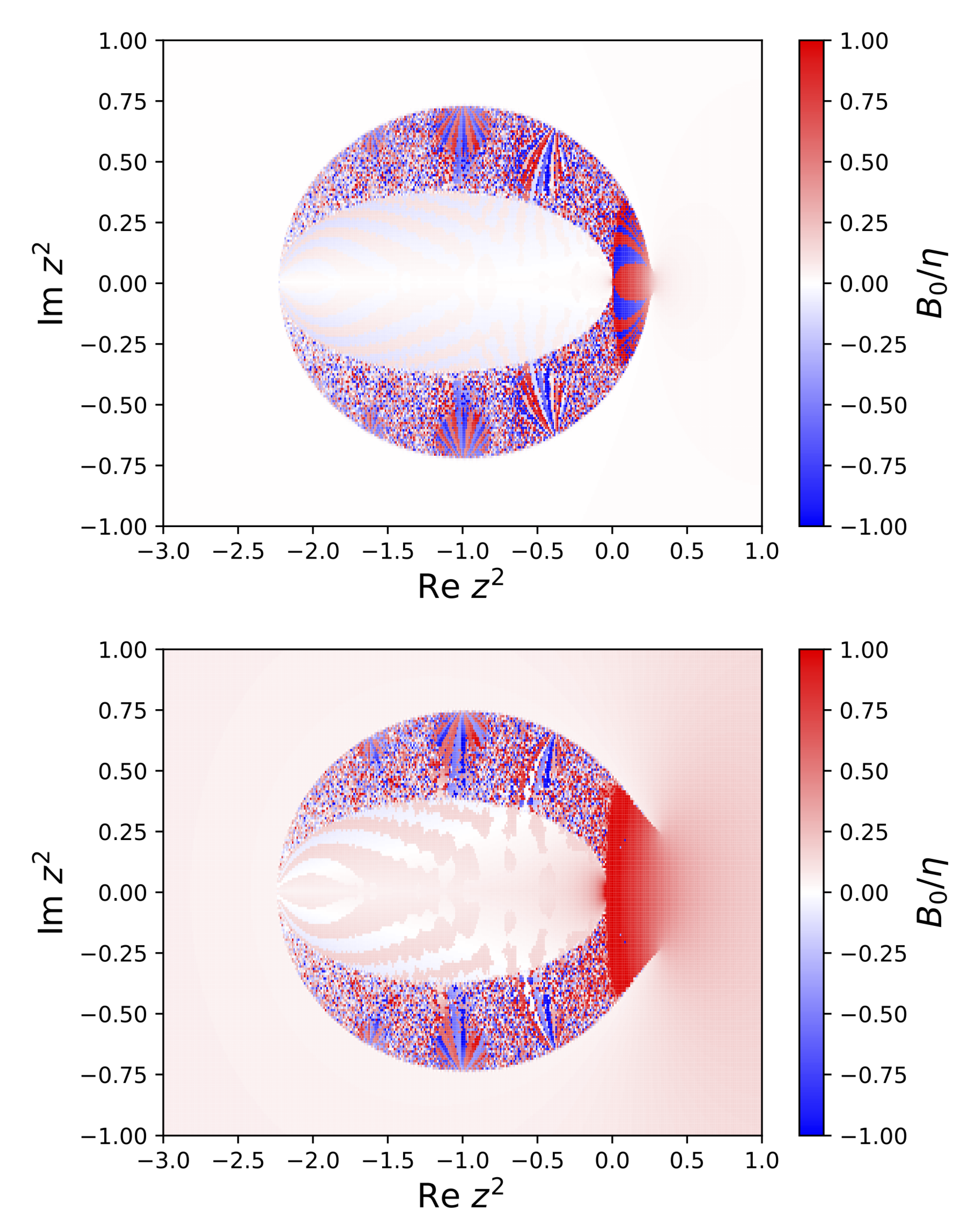
We start our iteration from the non-interacting solution (, ) and treat , as one would consider the constant c for the Mandelbrot set . For the moment, this reduces the number of independent variables from three () to two. The result of such an iteration is shown in Figure 1 for the real part of the scalar gap B at two different bare-quark masses of 10 MeV and 100 MeV, respectively.
Unlike the Mandelbrot fractal, this fractal does not diverge; chaos exhibits in domains in which the gaps for infinitesimal changes of energy and momentum take vastly different but finite values in a seemingly random pattern. This fractal region is contained within an almost perfectly shaped ellipsoid, which we fit accordingly with
differs slightly for MeV MeV and for MeV MeV. The inner almond shape with the less obvious chaotic behavior is well approximated by the same function with MeV for MeV, and MeV for MeV. As for the Mandelbrot set, one would be ill advised to understand these figures as a valid representation of the fractal; the appearance of the fractal changes with each new iteration. We identify regions with identical periodicity, ranging from a stable, period one solution in the region outside of the covering ellipse over a period two region within the almond shape, up to higher and higher periodicity in between these two regions. This is illustrated in Figure 2 for MeV for a periodicity of up to ten.
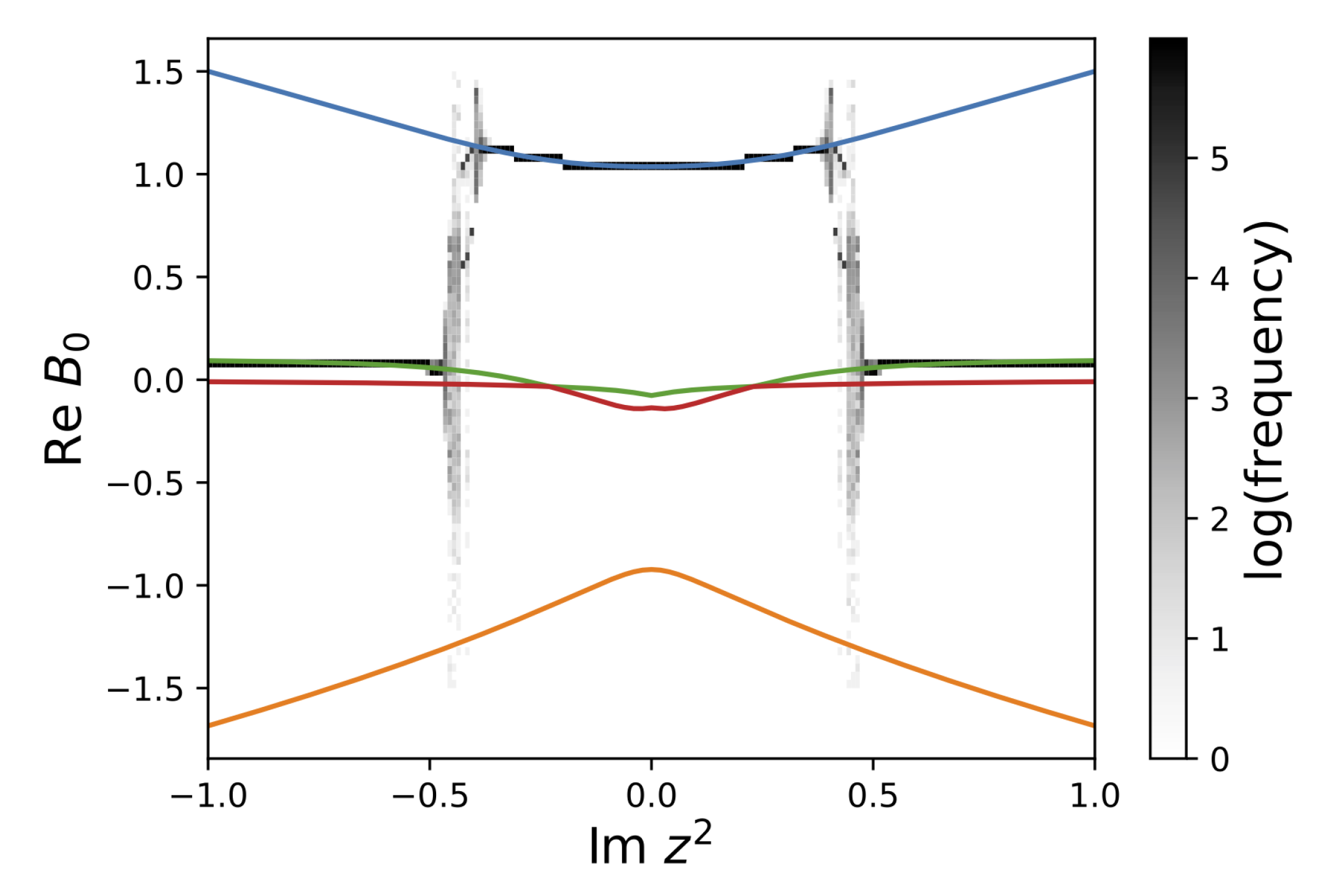
Keeping in mind that the analytic gap equations possess four distinct solutions, it seems interesting that there is an extended stable domain (periodicity one) which favors one, and only one solution. We follow the gap solution along a vertical path at fixed and vary . For reasons which become more clear at a later stage, we chose MeV. Along this line, one notices that one passes from an outer stable region into an inner stable region by traversing a small chaotic domain. This is illustrated in Figure 3. As within this chaotic domain the value of the gap function can change with each iteration, we plot all obtained values of over 300 iterations in gray scale according to how frequently a particular solution has been obtained. Evidently, there is a transition between two distinct analytic solutions of the non-iterated fourth-order polynomial gap equations. This result seems remarkable if one recalls how one would usually deal with different gap solutions for a given model: each solution is understood as a distinct phase, then one examines the stability of each individual solution and picks the energetically favored solution as the physical one. Upon iteration, we are lead to a different conclusion. Although each of the analytic solutions indeed is a solution of the gap equations, only one of them can be stable upon iteration at a given energy and momentum. However, the stable iterative solution over a finite range of energies can switch between distinct analytic solutions. It is further remarkable that the iteratively stable solution is massive (similar to the Wigner solution) when low and massless (similar to the Nambu solution) at high energy. Amongst all the possibilities chaos seems to offer, this seems a very reasonable one. While the exact meaning is unclear, it seems unlikely to be coincidence that iteration favors massive and massless solutions in precisely the energy regimes where confinement and asymptotic freedom are required.
The notion of analytic solutions describing different phases, however, is not supported from an iterative perspective; there is one, and only one, iterative solution to the gap equation.
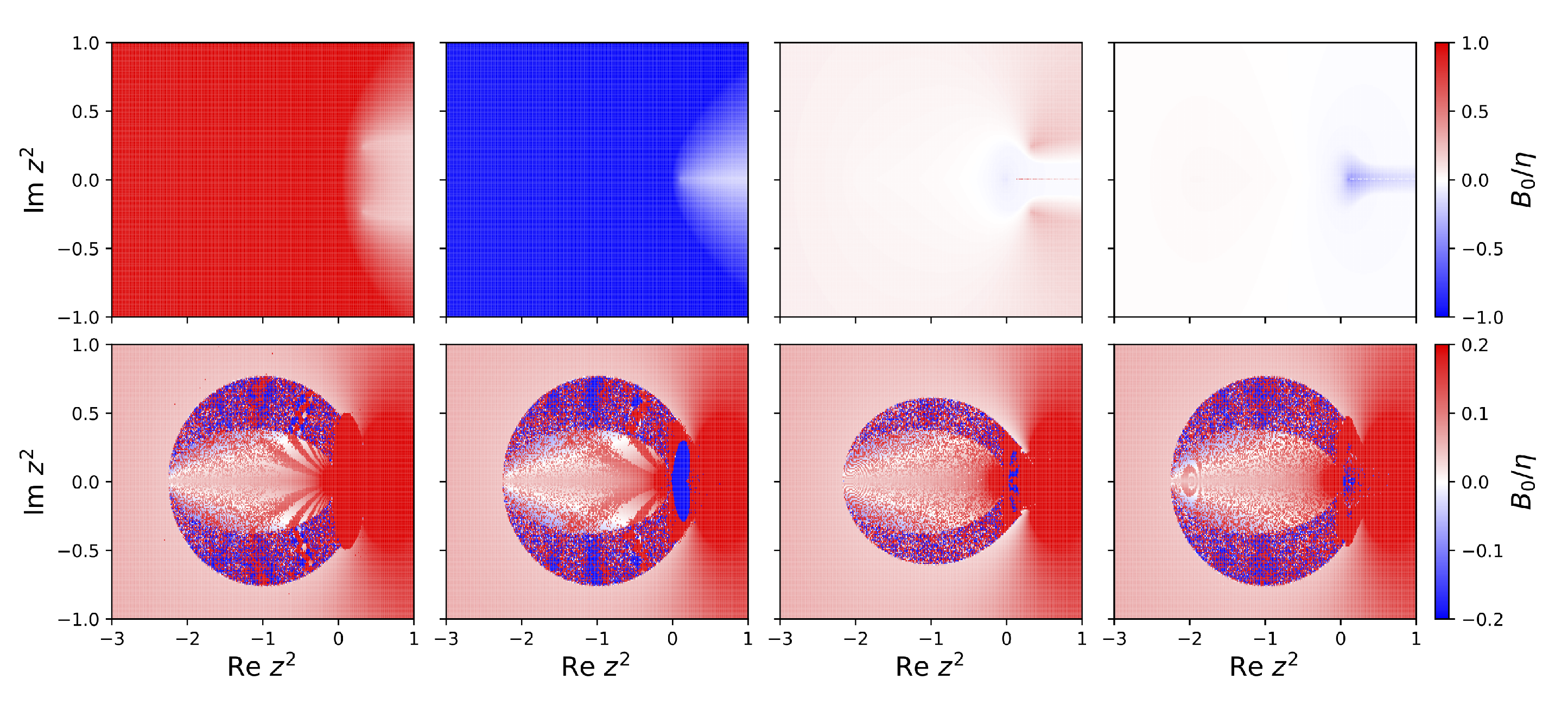
Before we go into a further interpretation of what this result implies, we wish to address a question related to the previous paragraph. Initially, we remarked that our iteration starts from the non-interacting solution . As we try to proceed as carefully as possible, let us investigate the iterative stability of the four analytic gap solutions as plotted in the upper panels of Figure 4, where we demonstrate again the real part of the mass gap. The lower panel of Figure 4 shows the result after 300 iterations of these algebraic solutions as an initial value. It is safe to say that none of them is stable under iteration. Further, there is a visibly favored solution at large values of , which does not depend on the initial gap that seeded the iteration. From a global perspective, the fractal keeps the general shape but shows differences for each different seed solution. This is to be expected and would happen in a similar fashion to the Mandelbrot set if the initial value was arbitrarily changed.
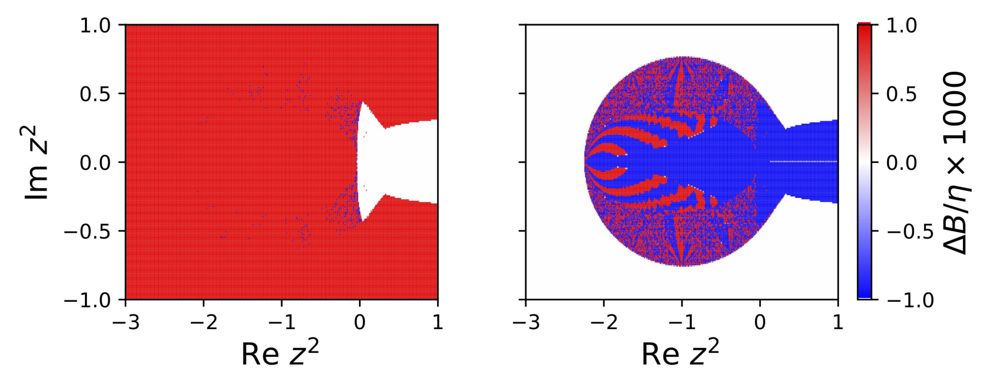
Comparing the iterations to the algebraic solutions of the gap equations in the upper panel of Figure 4, one can graphically identify which of them is stable under the iteration and in which domain. As observed, this is the case only for the positive mass-gap solutions 1 and 3 from Figure 4, as illustrated in Figure 5. In other words, although the chaotic domain will vary, the described features of Figure 3, with respect to the analytic gap solutions, do not critically depend on the chosen initial gap.
This iterative preference for one solution over the others seems to illustrate a case where Equation (1) favors a particular solution, while Equation (2) can be tuned to converge to any of the four analytic solutions. We take a moment, therefore, to discuss this further.
Precisely at an analytic solution, Equation (1) should be an identity so that with infinite precision, all of the solutions should stay precisely at their analytical value. However, any real solution will have at least some error, so that our numerical approximation is only in the neighborhood of the analytical solution. That is
where and represent the analytical solution and its numerical approximation, respectively. If we input into Equation (1), we obtain
Hence, the solution will be stable if and only if the functional’s derivative has a magnitude of less than 1.
Equation (2) resolves this so that if then after iteration
In this situation, we can always choose the sign (or phase) of such that near a specific analytical solution. Hence, we can make any of the analytical solutions stable by using Equation (2), but at most one such solution is stable under Equation (1), and that solution changes abruptly between very massive and nearly massless behavior in just the locations where we expect massive and massless behavior of the quarks. Whether this is a lucky coincidence, an actual effect of chaos, or a hint at something else in the true and final solution, is yet to be determined.
5. Mass Poles
Up to this point, we refrained from searching for meaning in our study. In spite of the fact that iterative mass gap solutions result in a large domain of chaotic behavior, which may or may not hide future surprises, we cannot help but wonder whether the switching between massive and mass-less gap solutions in the stable domains offers meaning. Before we go further, we want to recall that MN is considered to be a confining model. This is observed by the fact that the inverse propagator has no roots in the chirally broken phase and, therefore, the integration over the four-momentum does not pick up weight to generate a finite particle number. Hence, although confined quarks generate mass via chiral symmetry breaking, the absence of a mass pole results in the absence of a dispersion, viz., there is no explicit relation between specific momenta and energy. For the vacuum MN model, this is easily understood by the realization that in the Minkowski metric, has no real root if at any , . This running away of the mass in the chirally broken phase is exactly what happens in the MN model. However, as we have demonstrated in the previous section, the iteration erases the distinction between chirally broken and restored phases and suggests that instead there might be a discontinuous gap solution, which is confinement-like affected by dynamical chiral symmetry at small momenta, and at large momenta chirally unconfined-like and chirally restored. The transition between these domains is characterized by chaotic and unstable solutions (see Figure 3).
At finite chemical potential, the real poles of the propagator are represented by , with . We note that the shift of the pole due to the chemical potential should not be confused with the physical mass pole of the particle. This becomes evident if one considers an ideal non-interacting gas, with M being constant and real-valued. For the purpose of this study, we refer to the physical mass pole, defined by . From the definition , we identify the pole position in our contour plots as and for an ideal particle with constant and real M. This represents a vertical line in our plots, which does not depend on momentum and measures energy with increasing distance from the real axis. It shifts to higher with an increasing chemical potential.
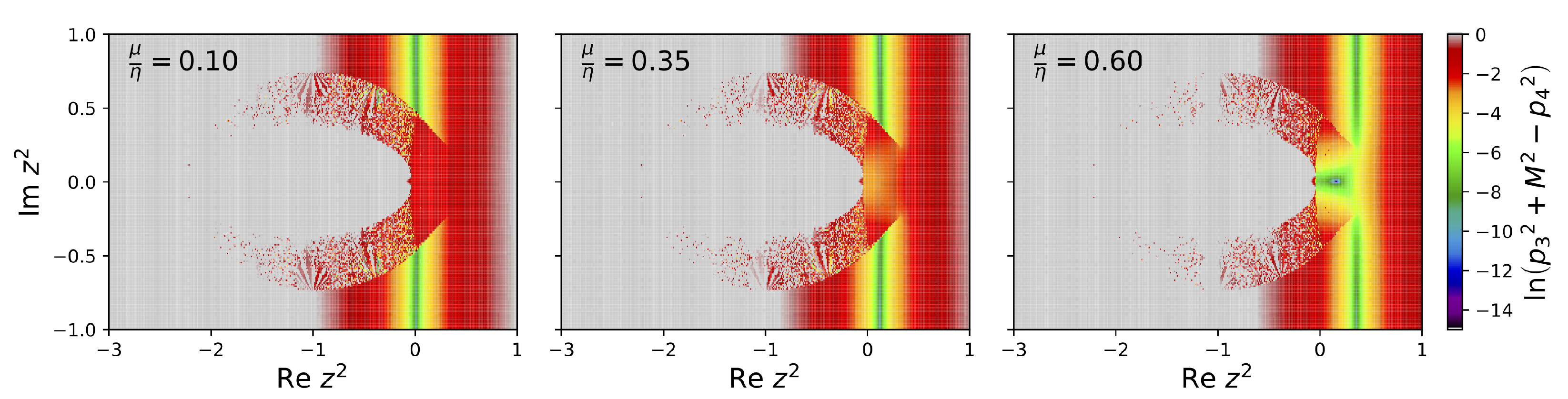
In Figure 6, we trace the physical mass pole in the Minkowski metric by plotting the logarithm of the quantity , which gives zero and hence a large negative logarithm at the physical mass pole. As the vertical axis does not depend on the mass (), a vertical pole line indicates constant dressed quark masses. We observe the absence of such a well ordered pole structure within the chaotic domain. Since the vertical axis is a measure of the particle energy at a fixed chemical potential, one can conclude that the transition to the massive solution (Figure 3) suppresses quasi-particle behavior in the infrared domain of the model. Again, we can trace the physical pole indicated by the vertical line and find , since the pole is found at . Following our elliptic fit of the outer boundary of the fractal domain, this allows one to determine the critical chemical potential where the infrared energy gap entirely disappears
We find MeV for MeV and MeV for MeV. At these chemical potentials and beyond, quarks can be considered as completely chirally restored.
In order to estimate when mass-pole states can be occupied, we determine at which chemical potential the energy and the Fermi energy or chemical potential turn equal, that is, when on the elliptic boundary of the fractal at the position of the physical mass pole with . We choose this scenario, as this is the critical potential starting from where the particle energy is larger than the chemical potential and thus large enough to populate quasi-particle states. This is the case when
and holds for the light quark with MeV at MeV, for the heavy quark with MeV at MeV.
Although this is not a rigorous statement, one can roughly relate the critical chemical potential for the transition from a chirally broken mass into the restored phase to the in-vacuum dressed-quark mass. In our case, the situation is a bit different. We estimate a hypothetical chirally broken quark vacuum mass based on the previous estimate of the critical potential for the complete disappearance of the infrared gap by setting them approximately equal. Relating as the onset of a deconfined chirally restored quark phase with an estimate of the constituent quark mass seems to provide rather reasonable results in comparison to other model calculations. This is interesting, considering that in the MN model, the vacuum mass at zero 4-momentum is defined by the coupling strength , which is of the order of 1 GeV.
It is noteworthy that our simple approach reproduces quantities related to the effective constituent masses at reasonable values. We state explicitly that in this model, constituent masses are nowhere realized for a physical particle, viz. an entity with a mass pole of that magnitude. We can compare the light quark critical chemical potential MeV with the deconfinement critical potential obtained within the MN model in a Euclidean metric with a value of 300 MeV [16] or with subsequent work based on a widened version of the effective gluon propagator [17], which predicts deconfinement at a chemical potential of 380 MeV. There is a satisfying agreement of these values with ours. We point out though, that both of these models are defined within a different metric, as slightly different bare quark masses and, most importantly, are based on entirely different assumptions. While the two previous papers employed distinct gap solutions and compare the pressure of the corresponding mass-less Wigner and massive Nambu phase, our approach results in only one gap solution which exhibits a transition from the Nambu to the Wigner phase through a chaotic domain, as depicted in Figure 3. Our quarks are either bare-mass quarks with poles or entities with a chaotic mass function, or a dressed quark mass different from the bare mass with no associated pole. In the latter case, there is a chaotic transition from dressed quark masses to bare quark masses with increasing energy.
6. Finite Interaction Width
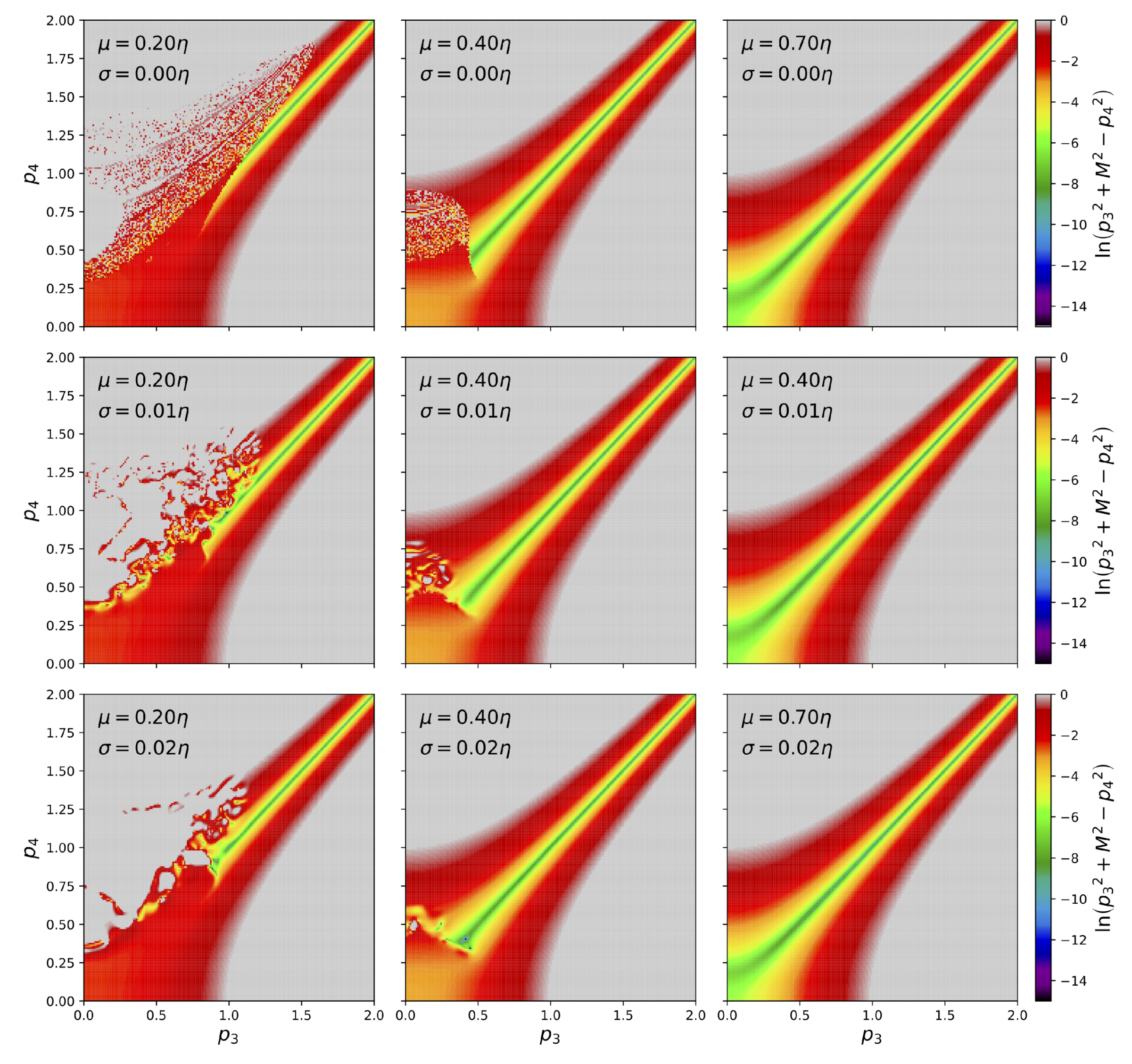
We begin the final section of this paper with a plot of the particle pole in an energy momentum space which we obtain by transforming to () coordinates under explicit choices of the chemical potential, as noted in Figure 7. Although this switch in representation does not provide additional information, we find it instructive to provide an actual dispersion relation obtained from the iterative approach. In this example, at a chemical potential of 700 MeV, no chaotic behavior is visible and the dispersion is exactly that of a free quark at bare-mass 100 MeV. With the decreasing chemical potential chaos, there emerges, at energies higher than that of the expected (now absent), the free particle dispersion. The actual dispersion branch is cut clean at some critical value (as we discussed in the previous section), thus illustrating our interpretation of the fractal boundary as the cause for a dynamical infrared cutoff, below which quarks are mass-pole-free.
Presently, we address a last question which relates to the fact that the MN model is based on the very particular choice of the effective gluon propagator as a -function in the four-momentum space. This is the reason that we could easily perform the presented study based on this Ansatz and the subsequent decoupling of momenta, which allows one to iterate point-wise for any given four-momentum without coupling to other momenta. This might raise the suspicion that momentum coupling could destroy the fractal structure we observed. In order to keep the simplicity of the gap equations but still obtain an idea about the stability of the emergent fractal, we averaged each point in our plane after each iteration step and thus mimicked some kind of momentum coupling. The averaging is based on Gaussian weights around a given point according to
where w is the width of the Gaussian. To further simplify, we assumed that the widening only happens in the direction of momentum and energy, i.e., there is no widening perpendicular to the momentum.
As observed in Figure 7, the separation into the chaotic pole-free and non-chaotic mass-pole domains remains, even when we change the momentum dependence of the gluon from a delta function to a Gaussian with a half width as much as 0.02 times the gluon mass. We find numerical evidence that this feature remains even with a width as much as 2% of the gluon mass, ≈ 20 MeV. This corresponds to a spatial width of about 10 fm, which is roughly one order of magnitude larger than the size of a proton. Based on this—certainly simplified—treatment of momentum coupling, we conclude that the statements we make in this paper may indeed survive a more complete treatment involving self-interactions with globally coupled momenta—which has been our main concern, prompting this final analysis.
7. Conclusions
As we have demonstrated, a strictly iterative solution of the MN gap equations results in fractal gap structures which can be characterized by the existence of three qualitatively very different, yet co-existing domains of a single and unique gap solution: a bare-mass quark quasi-particle domain with physical mass poles extending infinitely into the ultraviolet, a dressed-mass quark domain without mass poles and hence no quasi-particle interpretation in the infrared, and a chaotic domain of transition between the first two phases. Remarkably, the two non-chaotic domains correspond to distinct analytic solutions which would usually represent individual phases with either dynamically broken or restored chiral symmetry. The fractal approach offers an alternative to this separation which is rooted in the iterative nature of the gap equation.
Further, it is noteworthy that the iterative mass gap solution is always positive in the smooth, viz. non-chaotic domain of the fractal. The appearance of a chaotic boundary between two qualitatively different domains results in interesting properties:
- (I)
- The iterative approach provides an ultraviolet cut-off for the massive and mass-pole-free Nambu solution, as this solution appears only within the elliptic region of the () plane. Thus, the approach avoids the appearance of an infinitely increasing dressed-quark mass with increasing momentum and energy. In the MN model, this running mass results in the absence of mass poles for the massive gap solution and thus relates to confinement.
- (II)
- It provides an infrared cut-off for the bare-quark mass Nambu solution and thus ensures that quasi-particle states are not populated at a small chemical potential, although the quark can virtually exist as a quasi-particle with well defined dispersion.
- (III)
- Both cutoffs more or less coincide (as observed in Figure 5), although there is a transition region which is chaotic in nature. The resulting effective Nambu-UV/Wigner-IR cutoff depends dynamically on energy, momentum, bare mass, and chemical potential. As a side note, we add that plotting gap solutions in the () plane removes much of the dynamical arbitrariness and leaves the ratio of the bare mass m and coupling constant as the only ’true’ degree of freedom; viz., a change of the chemical potential would rescale the plot but cause no qualitative change, whereas plots such as Figure 1 indeed demonstrate ’the’ gap solution at an arbitrary chemical potential.
- (IV)
- Sufficiently large chemical potential bare-quark mass-pole states will form at energies which can be populated; thus, physical quarks can exist as quasi-particle excitations.
A mechanism with these properties can be interpreted as a deconfinement mechanism. The appearance of one, and only one, iterative solution of the MN gap equations bears a certain elegance. First, it is by the very fact that there is only one gap solution with expected properties, being the existence of only a positive mass gap, asymptotically restored chiral symmetry, and the absence or appearance of physical mass poles. Next, it builds on distinct solutions which one would obtain in the non-iterative approach but provides a new meaning by slicing them into a single new solution with the aforementioned properties.
A simple treatment of a widened, -like gluon interaction indicates that momentum coupling blurs chaotic domains but does not necessarily change the qualitative results we describe if the widening is moderate. As this study is an exploration and qualitative in nature, we look forward to further analyses of this perspective on understanding the confinement and the deconfinement transition as highly non-linear and, to a certain extent, with possibly chaotic phenomena.
Author Contributions
Conceptualization, T.K. and L.C.L.; methodology, T.K., L.C.L. and M.C.; numerical analysis, L.C.L. and M.C.; writing—original draft preparation, T.K. and L.C.L.; writing—review and editing, L.C.L. and M.C.; visualization: L.C.L. All authors have read and agreed to the published version of the manuscript.
Funding
M.C. acknowledges support from the Polish National Science Centre (NCN) under grant no. 2019/33/B/ST9/03059.
Data Availability Statement
No new data were created or analyzed in this study. Data sharing is not applicable to this article.
Acknowledgments
We are grateful to Prashanth Jaikumar, Pok Man Lo, and Craig D. Roberts for helpful comments and discussions, which helped us a great deal to find order in the chaos.
Conflicts of Interest
The authors declare no conflict of interest.
References
- Mandelbrot, B.B. Fractal Aspects of the Iteration of z→Λz(1-z) for Complex Λ and z. Ann. N. Y. Acad. Sci. 1980, 357, 249–259. [Google Scholar] [CrossRef]
- Kadanoff, L. Fractals: Where’s the Physics? Phys. Today 1986, 39, 6. [Google Scholar] [CrossRef]
- Stories, W.B. Mandelbrot about: Drawing; the Ability to Think in Pictures and Its Continued Influence. Available online: https://www.webofstories.com/play/benoit.mandelbrot/8 (accessed on 25 July 2020).
- Hofstadter, D.R. Energy levels and wave functions of Bloch electrons in rational and irrational magnetic fields. Phys. Rev. B 1976, 14, 2239–2249. [Google Scholar] [CrossRef]
- Kuhl, U.; Stöckmann, H.J. Microwave Realization of the Hofstadter Butterfly. Phys. Rev. Lett. 1998, 80, 3232–3235. [Google Scholar] [CrossRef]
- Roberts, C.D. Three Lectures on Hadron Physics. J. Phys. Conf. Ser. 2016, 706, 022003. [Google Scholar] [CrossRef]
- Horn, T.; Roberts, C.D. The pion: An enigma within the Standard Model. J. Phys. G 2016, 43, 073001. [Google Scholar] [CrossRef] [Green Version]
- Eichmann, G.; Sanchis-Alepuz, H.; Williams, R.; Alkofer, R.; Fischer, C.S. Baryons as relativistic three-quark bound states. Prog. Part. Nucl. Phys. 2016, 91, 1–100. [Google Scholar] [CrossRef] [Green Version]
- Burkert, V.D.; Roberts, C.D. Colloquium: Roper resonance: Toward a solution to the fifty year puzzle. Rev. Mod. Phys. 2019, 91, 011003. [Google Scholar] [CrossRef] [Green Version]
- Fischer, C.S. QCD at finite temperature and chemical potential from Dyson–Schwinger equations. Prog. Part. Nucl. Phys. 2019, 105, 1–60. [Google Scholar] [CrossRef] [Green Version]
- Roberts, C.D.; Schmidt, S.M. Reflections upon the Emergence of Hadronic Mass. Eur. Phys. J. Spec. Top. 2020, 229, 3319–3340. [Google Scholar] [CrossRef]
- Qin, S.X.; Roberts, C.D. Impressions of the Continuum Bound State Problem in QCD. Chin. Phys. Lett. 2020, 37, 121201. [Google Scholar] [CrossRef]
- Barabanov, M.Y.; Bedolla, M.A.; Brooks, W.K.; Cates, G.D.; Chen, C.; Chen, Y.; Cisbani, E.; Ding, M.; Eichmann, G.; Ent, R.; et al. Diquark Correlations in Hadron Physics: Origin, Impact and Evidence. Prog. Part. Nucl. Phys. 2021, 116, 103835. [Google Scholar] [CrossRef]
- Martínez, A.; Raya, A. Solving the Gap Equation of the NJL Model through Iteration: Unexpected Chaos. Symmetry 2019, 11, 492. [Google Scholar] [CrossRef] [Green Version]
- Munczek, H.J.; Nemirovsky, A.M. Ground-state mass spectrum in quantum chromodynamics. Phys. Rev. D 1983, 28, 181–186. [Google Scholar] [CrossRef]
- Klahn, T.; Roberts, C.D.; Chang, L.; Chen, H.; Liu, Y.X. Cold quarks in medium: An equation of state. Phys. Rev. C 2010, 82, 035801. [Google Scholar] [CrossRef] [Green Version]
- Chen, H.; Yuan, W.; Chang, L.; Liu, Y.X.; Klahn, T.; Roberts, C.D. Chemical potential and the gap equation. Phys. Rev. D 2008, 78, 116015. [Google Scholar] [CrossRef] [Green Version]
Figure 1.
Real part of the scalar gap B after 300 iterations starting from (top, bottom), and (10 MeV (top), 100 MeV (bottom)).
Figure 1.
Real part of the scalar gap B after 300 iterations starting from (top, bottom), and (10 MeV (top), 100 MeV (bottom)).

Figure 2.
Periodicity of the iterative mass gap solution at MeV. The outer, indigo region of the plot are absolutely stable under iteration, the inner almond shape has periodicity two, and the area in between exhibits chaos with increasing periodicity. For this plot, areas with periodicity larger than ten are plotted in black.

Figure 3.
Real part of the mass gap B at MeV. The color coding indicates how frequently a solution has been found over 300 iterations after the first 100 iterations which are sufficient to shape the fractal as seen. For reference, all analytic solutions to the polynomial gap equations are plotted in color. Iteration switches from massive solutions (blue) at small to bare-mass solutions (green) at larger values. Except for the chaotic transition domain, the iterative approach picks positive mass-gap solutions, only. Note, that the chaotic domain has solutions of periodicity of two and higher; it is truly unstable. Hence, we add a gray scale to measure the frequency of a particular solution over the final 300 iterations.

Figure 4.
Upper panel: Solutions of the polynomial gap equations for MeV. Each is plotted on a scale that most accentuates its structure. Solution 1 and 3 (from the left) are stable in some, mutually exclusive domains under iteration, as illustrated in Figure 3. Lower panel: After 300 iterations, using the corresponding solution of the polynomial gap equations from the upper panel as initial seed for the iteration. In the outer, non-chaotic domain, all four cases produce nearly identical results with positive mass gap only.

Figure 5.
Difference between gap solution 1 and 3 (from the left) in the top panel of Figure 4 and iterative solutions seeded with the non-interacting solution (, ) after 500 iterations. White domains show no difference between iterative solutions seeded with an analytical model solution or seeded with the non-interacting solution. Solution 2 and 4 show no agreement anywhere in the stable domain of periodicity one (not shown).

Figure 6.
Natural logarithm of for the iterative solution for MeV (top down) at quark-bare mass 100 MeV. The vertical line shaped by minimal negative values indicate a physical mass pole, viz. a quasi-particle. In the chaotic domain, this pole structure is absent, viz. the vertical line (or any distinct pole) pattern is absent. This implies an infrared energy gap, below which quarks show no quasi-particle properties. As the chemical potential increases, the quasi-particle pole line moves to the right and simultaneously decreases the gap, viz., the gap region without a pole traces the outer shape of the fractal. Once the chemical potential is sufficiently large, the gap closes entirely. Note that the absence of a mass pole does not imply that there is no mass gap solution, as illustrated in Figure 3.

Figure 7.
Plotted is the logarithm of the mass-pole condition , which shows a dispersion relation with distinct, chaos-induced infrared cut-off. With increasing chemical potential (; from left to right), the infrared cut-off decreases and eventually disappears. With increasing widening ( from top to bottom), chaotic domains blur but the observed IR cut-off remains.

Disclaimer/Publisher’s Note: The statements, opinions and data contained in all publications are solely those of the individual author(s) and contributor(s) and not of MDPI and/or the editor(s). MDPI and/or the editor(s) disclaim responsibility for any injury to people or property resulting from any ideas, methods, instructions or products referred to in the content. |
© 2023 by the authors. Licensee MDPI, Basel, Switzerland. This article is an open access article distributed under the terms and conditions of the Creative Commons Attribution (CC BY) license (https://creativecommons.org/licenses/by/4.0/).
Share and Cite
MDPI and ACS Style
Klähn, T.; Loveridge, L.C.; Cierniak, M. Chaos in QCD? Gap Equations and Their Fractal Properties. Particles 2023, 6, 470-484. https://doi.org/10.3390/particles6020026
AMA Style
Klähn T, Loveridge LC, Cierniak M. Chaos in QCD? Gap Equations and Their Fractal Properties. Particles. 2023; 6(2):470-484. https://doi.org/10.3390/particles6020026
Chicago/Turabian StyleKlähn, Thomas, Lee C. Loveridge, and Mateusz Cierniak. 2023. "Chaos in QCD? Gap Equations and Their Fractal Properties" Particles 6, no. 2: 470-484. https://doi.org/10.3390/particles6020026