Article

Parametrizations of Collinear and kT-Dependent Parton Densities in Proton

by
Nizami A. Abdulov
1,
Anatoly V. Kotikov
2,* and
Artem Lipatov
1,2
1
Skobeltsyn Institute of Nuclear Physics, Lomonosov Moscow State University, 119991 Moscow, Russia
2
Bogoliubov Laboratory of Theoretical Physics, Joint Institute for Nuclear Research, 141980 Dubna, Russia
*
Author to whom correspondence should be addressed.
Particles 2022, 5(4), 535-560; https://doi.org/10.3390/particles5040039
Submission received: 31 October 2022 / Revised: 21 November 2022 / Accepted: 22 November 2022 / Published: 28 November 2022
(This article belongs to the Special Issue 2022 Feature Papers by Particles’ Editorial Board Members)

Abstract

:
A new type of parametrization for parton distribution functions in the proton, based on their Q 2 -evolution at large and small x values, is constructed. In our analysis, the valence and nonsinglet parts obey the Gross–Llewellyn–Smith and Gottfried sum rules, respectively. For the singlet quark and gluon densities, momentum conservation is taken into account. Then, using the Kimber–Martin–Ryskin prescription, we extend the consideration to Transverse Momentum Dependent (TMD, or unintegrated) gluon and quark distributions in the proton, which currently plays an important role in a the number of phenomenological applications. The analytical expressions for the latter, valid for both low and large x, are derived for the first time.

1. Introduction

The parton (quark and gluon) distribution functions (PDFs) in the proton are a necessary part of any theoretical study performed within the quantum chromodynamics (QCD). They encode information on the non-perturbative structure of the proton and are directly related to the calculated cross sections (or other observables) via a certain QCD factorization theorem. The QCD evolution leads to their essential dependence on the probing scale Q 2 , which can be described by the Dokshitzer–Gribov–Lipatov–Altarelli–Parisi (DGLAP) equations [1,2,3,4]. Usually, the latter are solved numerically with leading (LO), next-to-leading (NLO) or even next-to-next-to-leading order (NNLO) accuracy, where a number of corresponding phenomenological parameters of initial parton distributions are fitted at HERA, LHC and fixed target experiments at various ( x , Q 2 ) ranges (several recent PDF fits, as well as the references to the previous studies, can be found [5,6,7,8,9,10,11,12,13,14,15,16,17,18,19,20,21,22]). Large uncertainties for many processes at the LHC originate, of course, mainly from our restricted knowledge of the parton distributions (see, for example, [23] and references therein). Thus, studying the proton PDFs from both theoretical and experimental points of view is an important and urgent task.
In the present paper, we continue with the idea [24] to present more information on the PDFs from the theoretical side. The approach consists of two basic steps. First, we find the asymptotics of solutions of the DGLAP equations for the parton densities at small and large values of the Bjorken variable x. Second, we combine these two solutions and then interpolate between them to obtain analytical expressions for PDFs over the full range of x.
In a sense, this is not a very new idea. A similar approach was proposed [25,26,27] about 50 years ago. However, in the present paper, the parametrizations are constructed in quite a different way. In particular, following [24], they include important subasymptotic terms which are fixed exactly by the momentum conservation and also by the Gross–Llewellyn–Smith and Gottfried sum rules (see [28,29], respectively). Such calculations will be performed for the first time providing the community with a new type of parametrization of gluon and quark densities in the proton valid at low and large x. Moreover, we extend our consideration [30,31] and derive analytical expressions for Transverse Momentum Dependent (TMD) parton distributions using the Kimber–Martin–Ryskin (KMR) framework [32,33,34]. These quantities are known to be a very suitable tool to investigate less inclusive processes which proceed at high energies with large momentum transfer and/or contain multiple hard scales (see, for example, review [35] and references therein). Our main motivation is that up until now, there are no analytical expressions for gluon and especially quark TMDs (both sea and valence) valid in a wide x region (in our previous study [30,31], only the small x limit was considered and a phenomenological model for the large x region was applied).
The analysis of the present paper is limited to LO in the perturbation theory, which is reasonable [36] for those processes at the LHC for which the NLO corrections are not known at present. Moreover, most phenomenological applications involving TMDs are currently performed at LO also (see, for example, [31,37,38,39,40] and references therein). On the other hand, the consideration of PDFs at LO is a necessary first step in studying PDFs and TMDs at higher orders. These higher order corrections can be treated like those from [27,41,42].
The outline of our paper is the following. In Section 2, we describe our theoretical input. Section 3 and Section 4 contain low x and large x PDF asymptotics. Parametrizations of parton densities, their properties and numerical results for PDFs are given in Section 5. Section 6 is devoted to TMD parton densities in the Kimber–Martin–Ryskin framework. Section 7 contains our conclusions. The most complicated calculations are presented in Appendices.

2. Theoretical Input

In this section, we briefly present the theoretical part of our analysis. The reader is referred to [43,44] for more details.
The deep-inelastic scattering (DIS) l + N l + X , where l and N are the incoming lepton and nucleon, and l is the outgoing lepton, in one of the basic processes for studying the nucleon structure. The DIS cross-section can be split to the lepton L μ ν and hadron F μ ν parts
d σ L μ ν F μ ν .
The lepton part L μ ν is evaluated exactly, while the hadron one, F μ ν , can be presented in the following form
F μ ν = g μ ν + q μ q ν q 2 F 1 ( x , Q 2 ) + p μ + ( p q ) q 2 q μ p ν + ( p q ) q 2 q ν F 2 ( x , Q 2 ) + i ε μ ν α β p α p β x q 2 F 3 ( x , Q 2 ) + ,
where the symbol … stands for those parts which depend on the nucleon spin. The functions F k ( x , Q 2 ) with k = 1 , 2 and 3 are the DIS structure functions (SFs) and q and p are the photon and parton momenta. Moreover, the two variables
Q 2 = q 2 > 0 , x = Q 2 2 ( p q )
determine the basic properties of the DIS process. Here, Q 2 is the “mass” of the virtual photon and/or Z / W boson, and the Bjorken variable x ( 0 < x < 1 ) is the part of the hadron momentum carried by the scattering parton (quark or gluon).

2.1. Mellin Transform

The Mellin transform diagonalizes the Q 2 evolution of the parton densities. In other words, the Q 2 evolution of the Mellin moment with a certain value n does not depend on the moment with another value n .
The Mellin moments M k ( n , Q 2 ) of the SF F k ( x , Q 2 )
M k ( n , Q 2 ) = 0 1 d x x n 2 F k ( x , Q 2 )
can be represented as the sum
M k ( n , Q 2 ) = a = q , q ¯ , g C k a ( n , Q 2 / μ 2 ) A a ( n , μ 2 ) ,
where C k a ( n , Q 2 / μ 2 ) are the coefficient functions and A a ( n , μ 2 ) = < N | O μ 1 , , μ n a | N > are the matrix elements of the Wilson operators O μ 1 , , μ n a , which in turn are process-independent.
Phenomenologically, the matrix elements A a ( n , μ 2 ) are equal to the Mellin moments of the PDFs f a ( x , μ 2 ) , where f a ( x , μ 2 ) are the distributions (all parton densities are multiplied by x, i.e., in LO the structure functions are some combinations of the parton densities) of quarks ( a = q i ), antiquarks ( a = q ¯ i ) with i = 1 6 and gluons ( a = g ), i.e.,
A a ( n , μ 2 ) f a ( n , μ 2 ) = 0 1 d x x n 2 f a ( x , μ 2 ) .
The coefficient functions C k a ( n , Q 2 / μ 2 ) are represented by
C k a ( n , Q 2 / μ 2 ) = 0 1 d x x n 2 C ˜ k a ( x , Q 2 / μ 2 )
and responsible for the relationship between SFs and PDFs. Indeed, in the x-space the relation (5) is replaced by
F k ( x , Q 2 ) = a = q , q ¯ , g C ˜ k a ( x , Q 2 / μ 2 ) f a ( x , μ 2 ) ,
where ⊗ denotes the Mellin convolution
f 1 ( x ) f 2 ( x ) x 1 d y y f 1 ( y ) f 2 x y .
Applying (5) and (8), one can fit the shapes of PDFs f a ( x , μ 2 ) , which are process-independent and use them later for other processes. Note that the factorization scale μ 2 is often taken as μ 2 = Q 2 . Here, we will follow this choice.

2.2. Quark Densities

The distributions of the u and d quarks contain the valence and sea parts:
f q 1 f u = f u V + f u S , f q 2 f d = f d V + f d S .
The distributions of the other quark flavors and of all the antiquarks contain the sea parts only:
f q j = f q j S , ( j = 3 6 ) , f q ¯ i = f q ¯ i S ( i = 1 6 ) .
It is useful to define combinations [42] of quark densities (here, we consider all quark flavors. In fact, heavy quarks factorize out when Q 2 becomes less then their masses, and we should exclude them from the Q 2 -region): the valence part f V , the sea one f S and the singlet one f S I :
f V = f u V + f d V , f S = i = 1 6 f q i S + f q ¯ i S , f S I = i = 1 6 f q i + f q ¯ i = f V + f S .
Since the PDFs, which contribute to the structure functions, are accompanied by some numerical factors, there are also nonsinglet parts
f Δ i j = f q i + f q ¯ i f q j + f q ¯ j ,
which contain the difference in the densities of quarks and antiquarks with different values of charges.
As an example, we consider electron-proton scattering, where the corresponding SF has the form
F 2 e p ( x , Q 2 ) = i = 1 6 e i 2 f q i ( x , Q 2 ) + f q ¯ i ( x , Q 2 ) .
In a four-quark case (when b and t quarks are separated out), we will have [42]
F 2 e p ( x , Q 2 ) = 5 18 f S I ( x , Q 2 ) + 1 6 f Δ ( x , Q 2 ) ,
where
f Δ = q i = u , c f q i ( x , Q 2 ) + f q ¯ i ( x , Q 2 ) q i = d , s f q i ( x , Q 2 ) + f q ¯ i ( x , Q 2 ) .

2.3. DGLAP Equations

The PDFs obey the DGLAP equations [1,2,3,4]:
d d ln Q 2 f i ( x , Q 2 ) = 1 2 b γ N S ( x ) f i ( x , Q 2 ) , i = N S , V , d d ln Q 2 f a ( x , Q 2 ) = 1 2 b γ a b ( x ) f b ( x , Q 2 ) , a , b = S I , g ,
where γ i ( x ) and γ a b ( x ) are so-called splitting functions. Anomalous dimensions (ADs) γ a b ( n ) of the twist-two Wilson operators O μ 1 , , μ n a in the brackets b are the Mellin transforms of the corresponding splitting functions
γ a b ( n ) = 0 1 d x x n 2 γ a b ( x ) , f a ( n , μ 2 ) = 0 1 d x x n 2 f a ( x , μ 2 ) .
At LO of perturbation theory, ADs
γ a b ( n ) have the following form [42]:
γ a b ( n ) = a s ( Q 2 ) γ a b ( 0 ) ( n ) , γ N S ( 0 ) ( n ) = γ q q ( 0 ) ( n ) , a s ( Q 2 ) = α s ( Q 2 ) 4 π = 1 β 0 ln ( Q 2 / Λ LO 2 ) , γ N S ( 0 ) ( n ) = γ q q ( 0 ) ( n ) = 8 C F S 1 ( n ) 3 4 1 2 n ( n + 1 ) , γ q g ( 0 ) ( n ) = 4 f n 2 + n + 2 n ( n + 1 ) ( n + 2 ) , γ g q ( 0 ) ( n ) = 4 C F n 2 + n + 2 n ( n 2 1 ) , γ g g ( 0 ) ( n ) = 8 C A S 1 ( n ) 11 12 1 n ( n 1 ) 1 ( n + 1 ) ( n + 2 ) + 4 f 3 ,
where C A = N , C F = ( N 2 1 ) / ( 2 N ) for SU(N) group and f is the number of active (massless) quarks and
S 1 ( n ) = m = 1 n 1 m = Ψ ( n + 1 ) + γ E ,
with Euler Ψ -function and Euler constant γ E .
In the Mellin moment space, the DGLAP equation becomes the standard renormalization group equation. At LO we have
d d ln Q 2 f i ( n , Q 2 ) = a s ( Q 2 ) 2 γ N S ( 0 ) ( n ) f i ( n , Q 2 ) , i = V , N S ,
d d ln Q 2 f a ( n , Q 2 ) = a s ( Q 2 ) 2 b = S I , G γ a b ( 0 ) ( n ) f b ( n , Q 2 ) , a = S I , g .
To solve (22), it is more convenient to move to the ± components [42,45], that leads to the diagonal form:
d d ln Q 2 f ± ( n , Q 2 ) = a s ( Q 2 ) 2 γ ± ( 0 ) ( n ) f ± ( n , Q 2 ) ,
where
γ ± ( 0 ) ( n ) = 1 2 γ q q ( 0 ) ( n ) + γ g g ( 0 ) ( n ) ± ( γ q q ( 0 ) ( n ) γ g g ( 0 ) ( n ) ) 2 + 4 γ q g ( 0 ) ( n ) γ g q ( 0 ) ( n ) .
The solutions of (21) and (23) have the following form:
f a ( n , μ 2 ) = f a ( n , Q 0 2 ) e d a ( n ) s , a = V , N S , ± ,
where Q 0 2 is some initial scale and
d a ( n ) = γ a ( 0 ) ( n ) 2 β 0 , s = ln ln ( Q 2 / Λ 2 ) ln ( Q 0 2 / Λ 2 ) .
The singlet quark and gluon densities can be expressed through their “±” components as
f a ( n , Q 2 ) = f a , + ( n , Q 2 ) + f a , ( n , Q 2 ) , f a , ± ( n , Q 2 ) = f a , ± ( n , Q 0 2 ) e d ± ( n ) s ,
where
f q , + ( n , Q 0 2 ) = f q ( n , Q 0 2 ) f q , ( n , Q 0 2 ) , f q , ( n , Q 0 2 ) = f q ( n , Q 0 2 ) α n + f q ( n , Q 0 2 ) β n , f g , ( n , Q 0 2 ) = f g ( n , Q 0 2 ) f g , + ( n , Q 0 2 ) , f q , + ( n , Q 0 2 ) = f g ( n , Q 0 2 ) α n f q ( n , Q 0 2 ) ϵ n ,
and
α n = γ q q ( 0 ) ( n ) γ + ( 0 ) ( n ) γ ( 0 ) ( n ) γ + ( 0 ) ( n ) , β n = γ q g ( 0 ) ( n ) γ ( 0 ) ( n ) γ + ( 0 ) ( n ) , ϵ n = γ g q ( 0 ) ( n ) γ ( 0 ) ( n ) γ + ( 0 ) ( n ) .

2.4. Special Cases

A special case of parton evolution is the case n = 1 for the valence part, which corresponds to the number N V of structural quarks in a considered hadron. For example, for a proton N V = 3 . So, we have
0 1 d x 1 x f V ( x , μ 2 ) = N V ,
which is the so-called Gross-Llewellyn-Smith sum rule [28].
Indeed, for this case, γ N S ( 0 ) ( n = 1 ) = 0 and
f a ( n = 1 , Q 2 ) = f a ( n = 1 , Q 0 2 ) , a = V , N S .
For the NS part, the corresponding sum rule, so-called Gottfried sum rule [29], is written as
0 1 d x 1 x f N S ( x , Q 2 ) = N N S ( Q 2 ) = 3 I G ( Q 2 ) ,
with [46]
I G ( Q c 2 ) = 0.705 ± 0.078 , Q c 2 = 4 GeV 2 .
We note that the result (32) is correct in a case of flavor-symmetric sea. Moreover, I G ( Q 2 ) has only very weak Q 2 -dependence (see [47]), which comes beyond LO from the so-called analytic continuation [47,48,49] of the corresponding Wilson coefficients. So, the values of the Gottfried sum rule [29] can be taken below as
I G ( Q 2 ) I G ( Q c 2 ) = 0.705 .
For the sea quark and gluon densities the special case is n = 2 , that corresponds to the conservation of the total momentum carried by quarks and gluons, i.e.,
0 1 d x f S I ( x , Q 2 ) + f g ( x , Q 2 ) = 0 1 d x f S I ( x , Q 0 2 ) + f g ( x , Q 0 2 ) = 1 ,
i.e.,
f S I ( n = 2 , Q 2 ) + f g ( n = 2 , Q 2 ) = f S I ( n = 2 , Q 0 2 ) + f g ( n = 2 , Q 0 2 ) ) = 1 .
Let us consider the case n = 2 more accurately. We have
γ q q ( 0 ) ( n = 2 ) = γ g q ( 0 ) ( n = 2 ) = 16 C F 3 , γ g g ( 0 ) ( n = 2 ) = γ q g ( 0 ) ( n = 2 ) = 4 f 3 ,
and thus,
γ ( 0 ) ( n = 2 ) = 0 , γ + ( 0 ) ( n = 2 ) = 4 3 4 C F + f , α n = 2 = β n = 2 = 1 ϵ n = 2 = f 4 C F + f .
Using these values, we obtain
f S I , ( 2 , Q 2 ) = f 4 C F + f f S I ( 2 , Q 0 2 ) + f g ( 2 , Q 0 2 ) e d ( n = 2 ) s = f 4 C F + f , f g , ( 2 , Q 2 ) = 4 C F 4 C F + f f S I ( 2 , Q 0 2 ) + f g ( 2 , Q 0 2 ) e d ( n = 2 ) s = 4 C F 4 C F + f ,
because f S I ( 2 , μ 0 2 ) + f g ( 2 , μ 0 2 ) = 1 and d ( n = 2 ) = γ ( n = 2 ) / ( 2 β 0 ) = 0 . Thus, the “−”-components are Q 2 -independent. Moreover,
f S I , ( 2 , Q 2 ) + f g , ( 2 , Q 2 ) = f S I ( 2 , Q 0 2 ) + f g ( 2 , Q 0 2 ) = 1 ,
i.e., the sum of the “−” components of the singlet and gluon densities is responsible for the momentum conservation. For the “+” components we have
f S I , + ( n , Q 2 ) = 1 4 C F + f 4 C F f S I ( 2 , Q 0 2 ) f f g ( 2 , Q 0 2 ) e d + ( n = 2 ) s , f g , + ( n , Q 2 ) = 1 4 C F + f f f g ( 2 , Q 0 2 ) 4 C F f S I ( 2 , Q 0 2 ) e d + ( n = 2 ) s
and thus,
f S I , + ( 2 , Q 2 ) + f g , + ( 2 , Q 2 ) = 0 ,
i.e., the sum of the “+” components of the singlet and gluon densities is exactly zero.

3. Low x Asymptotics

According to (12), the singlet quark density f S I ( x , Q 2 ) contains the valence part f V ( x , Q 2 ) and the sea part f S ( x , Q 2 ) .

3.1. Nonsinglet and Valence Parts

At small-x values, the NS and valence parts have the following asymptotics [25,26,50,51]:
f i ( x ) A i ( s ) x λ i , i = V , N S ,
where the variable s is defined in Equation (26) and
A i ( s ) = A i ( 0 ) e d V ( 1 λ i ) s , A i ( 0 ) A i , d V ( n ) = γ N S ( 0 ) ( n ) 2 β 0 ,
λ i and A i ( 0 ) are free parameters and Ψ ( n + 1 ) is the Euler Ψ -function. It follows from the Regge calculus that the constant λ i 0.3 ÷ 0.5 . Moreover, the Q 2 evolution of this parton density shows that λ i must be Q 2 independent [25,26].

3.2. Singlet Part

It was pointed out [52] that HERA small-x data can be well interpreted in terms of the so-called doubled asymptotic scaling (DAS) phenomenon related to the asymptotic behavior of the DGLAP evolution discovered many years ago [53]. The study [52] was extended [54,55,56] to include the finite parts of anomalous dimensions of Wilson operators and Wilson coefficients (in the standard DAS approximation [53] only the AD singular parts were used) (see review [43] and discussions therein). This leads to predictions [55,56] of the small-x asymptotic form of PDFs in the framework of the DGLAP dynamics, which were obtained starting at some Q 0 2 with the flat function
f a ( x , Q 0 2 ) = A a ,
where A a are free parameters that have to be determined from the data. We refer to the approach of [54,55,56] as generalized DAS approximation. In this approach, the flat initial conditions (45) determine the basic role of the AD singular parts as in the standard DAS case, whereas the contributions coming from AD finite parts and Wilson coefficients can be considered as corrections which are, however, important for achieving better agreement with experimental data.
The generalized DAS approach has been successfully used to fit the experimental data for F 2 and F 2 c SFs (see Refs. [52,55,56,57,58,59,60,61,62], respectively). In addition, it helps to extract gluon density and F L SF from experimental data of F 2 and its derivative with respect to Q 2 (see [63,64] and [65,66,67], respectively), to estimate the charm part of F L [68] and, finally, it leads to useful links between SFs [69,70,71]. Moreover, the generalized DAS approach provides the correct Q 2 - dependence of F 2 slope [72] and reasonable asymptotics for nucleon PDFs [73,74]. All the described cases take place for small values of the Bjorken variable x.
The generalized DAS approach also leads to simple and convenient low-x forms for non-integrated quark and gluon densities [30,31], the application of which will be extended to the entire area x in Section 6.
Hereafter, we consider for simplicity only the LO approximation (both the LO and NLO results and their applications can be found in [55,56]). The small-x asymptotic expressions for the sea quark and gluon densities f a ( x , μ 2 ) can be written as follows:
f a ( x , Q 2 ) = f a + ( x , Q 2 ) + f a ( x , Q 2 ) , f g + ( x , Q 2 ) = A g + I ¯ 0 ( σ ) e d ¯ + s + O ( ρ ) , A g + = A g + C A q , C = C F C A = 4 9 , f q + ( x , Q 2 ) = A q + I ˜ 1 ( σ ) e d ¯ + s + O ( ρ ) , A q + = φ 3 A g + , φ = f C A = f 3 , f g ( x , Q 2 ) = A g e d s + O ( x ) , A g = C A q , f q ( x , Q 2 ) = A q e d s + O ( x ) ,
where C A = N c , C F = ( N c 2 1 ) / ( 2 N c ) for the color S U ( N c ) group, I ¯ ν ( σ ) and I ˜ ν ( σ ) ( ν = 0 , 1 ) are the combinations of the modified Bessel functions (at s 0 , i.e., μ 2 Q 0 2 ) and usual Bessel functions (at s < 0 , i.e., μ 2 < Q 0 2 ):
I ˜ ν ( σ ) = ρ ν I ν ( σ ) , if s 0 ; ( ρ ˜ ) ν J ν ( σ ˜ ) , if s < 0 . , I ¯ ν ( σ ) = ρ ν I ν ( σ ) , if s 0 ; ρ ˜ ν J ν ( σ ˜ ) , if s < 0 . I ν ( σ ) = m = 0 1 k ! ( k + ν ) ! σ 2 k + ν , J ν ( σ ) = m = 0 ( 1 ) k k ! ( k + ν ) ! σ 2 k + ν ,
where I ¯ 0 ( σ ) = I ˜ 0 ( σ ) and
σ = 2 d ^ + s ln 1 x , ρ = σ 2 ln ( 1 / x ) , σ ˜ = 2 d ^ + s ln 1 x , ρ ˜ = σ ˜ 2 ln ( 1 / x ) ,
and
d ^ + = 4 C A β 0 = 12 β 0 , d ¯ + = 1 + 4 f ( 1 C ) 3 β 0 = 1 + 20 f 27 β 0 , d = 4 C f 3 β 0 = 16 f 27 β 0 ,
are the singular and regular parts of the anomalous dimensions and β 0 = 11 ( 2 / 3 ) f is the first coefficient of the QCD β -function in the MS ¯ -scheme. The results for the parameters A a and Q 0 2 can be found in [61]; they were obtained for α s ( M Z ) = 0.1168 .
It is convenient to have the following expressions:
β 0 d ^ + = 4 C A , β 0 d ¯ + = C A 3 11 + 2 φ ( 1 2 C ) , β 0 d = 4 C f 3 = 4 C F φ 3 .

4. Large x Asymptotics

The large x asymptotics of the valence, nonsinglet and sea quark densities have the following form (see [25,26,50,51] and Appendix A):
f i ( x , Q 2 ) B i ( s ) Γ ( 1 + ν i ( s ) ) ( 1 x ) ν i ( s ) , i = N S , V , f a ( x , Q 2 ) = ± f a , ± ( x , Q 2 ) , a = q , g , f q , ( x , Q 2 ) B ( s ) Γ ( 1 + ν ( s ) ) ( 1 x ) ν ( s ) , f g , ( x , Q 2 ) K Γ ( 2 + ν ( s ) ) B ( s ) ln ( 1 / ( 1 x ) ) + c ^ + Ψ ( ν + 2 ) ( 1 x ) ν ( s ) + 1 , f g , + ( x , Q 2 ) B + ( s ) Γ ( 1 + ν + ( s ) ) ( 1 x ) ν + ( s ) , f q , + ( x , Q 2 ) K + Γ ( 2 + ν + ( s ) ) B + ( s ) x ln ( 1 / ( 1 x ) ) + c ^ + Ψ ( ν + + 2 ) ( 1 x ) ν + ( s ) + 1 ,
where
ν i ( s ) = ν i ( 0 ) + r i s , r i = 4 C i β 0 , B i ( s ) = B i ( 0 ) e p i s , p i = r i γ E + c ^ i , i = N S , V , ± ,
with B i ( 0 ) and ν i ( 0 ) being free parameters, γ E is the Euler constant and
C + = C A , c ^ + = β 0 4 C A = 11 2 φ 12 , C j = C F , c ^ j = 3 4 , j = V , N S , K + = f 2 ( C A C F ) , K = C F 2 ( C A C F ) , c ^ = γ E + C A c ^ + C F c ^ C A C F
The constant ν i ( 0 ) can be estimated from the quark counting rules [75,76,77] as
ν j ( 0 ) 3 , j = V , N S , , ν + ( 0 ) = ν j ( 0 ) + 1 .
The relation ν + ( s ) = ν ( s ) + 1 leads to smallness of the term f q , + ( x , Q 2 ) . So, at large x we have
f q , + ( x , Q 2 ) 0 a n d , t h u s , f q ( x , Q 2 ) f q , ( x , Q 2 ) .
Moreover, the expressions (51) and (52) demonstrate fall of the parton densities at large x when Q 2 increases.

5. Parametrizations

Here, we present parametrizations of the nonsinglet and singlet quark and gluon densities constructed similar to ones obtained earlier [24] in the valence case.

5.1. Nonsinglet and Valence Parts

The nonsinglet and valence quark parts f i ( x , Q 2 ) , where i = V , N S , can be represented in the following form (similar studies were carried out in [78,79,80] (see also the review [43])):
f i ( x , Q 2 ) = A i ( s ) x λ i ( 1 x ) + B i ( s ) x Γ ( 1 + ν i ( s ) ) + D i ( s ) x ( 1 x ) ( 1 x ) ν i ( s ) ,
which is constructed as a combination of the small x and large x asymptotics and an additional term proportional to D i ( s ) , which is subasymptotic in both of these regions. The Q 2 -dependence of the parameters in (56) is given by (51) and (44). The Q 2 -dependence of magnitude D i ( s ) is determined by the corresponding sum rules (see below).

5.2. Sea and Gluon Parts

The sea and gluon parts can be represented as combinations of the ± terms:
f j ( x , Q 2 ) = ± f j , ± ( x , Q 2 ) , j = q , g , f q , ( x , Q 2 ) = A q e d s ( 1 x ) m q , + B ( s ) x Γ ( 1 + ν ( s ) ) + D ( s ) x ( 1 x ) ( 1 x ) ν ( s ) , f g , ( x , Q 2 ) = A g e d s ( 1 x ) m g , + K Γ ( 2 + ν ( s ) ) B ( s ) x ln ( 1 / ( 1 x ) ) + c ^ + Ψ ( ν + 2 ) ( 1 x ) ν ( s ) + 1 , f g , + ( x , Q 2 ) = A g + I ¯ 0 ( σ ) e d ¯ + s ( 1 x ) m g , + + B + ( s ) x Γ ( 1 + ν + ( s ) ) + D + ( s ) x ( 1 x ) ( 1 x ) ν + ( s ) , f q , + ( x , Q 2 ) = A q + I ˜ 1 ( σ ) e d ¯ + s ( 1 x ) ν + ( s ) + m q , + + 1 ,
where K and c ^ are shown in (53). We note that one can set m q , = m g , + = 2 and m q , + = m g , = 1 . In this case, small-x asymptotics is suppressed for large x in comparison with the subasymptotic behavior of D ± ( x ) . Moreover, the small-x asymptotics will contain the same powers of the factor ( 1 x ) for quarks and gluons.
We would like to note that the valence quarks contribute to the “−”-component but not to “+”-one. So,
f S I ( x , Q 2 ) = f S I , ( x , Q 2 ) + f S I , + ( x , Q 2 ) , f S I , ( x , Q 2 ) = f q , ( x , Q 2 ) + f V ( x , Q 2 ) , f S I , + ( x , Q 2 ) = f q , + ( x , Q 2 ) .
The parameters involved in (56)–(58) can be fitted, for example, from the comparison with known parametrizations of the NNPDF group [7] and/or taking into account the sum rules shown in the next section.

5.3. Properties of Parameterizations

The obtained above parametrizations of parton distributions in the proton must obey sum rules given by (30) and (32).

5.3.1. Gross–Llewellyn–Smith and Gottfried Sum Rules

Additional relations between the parameters in (56) stems from the LO Gross–Llewellyn–Smith sum rule [28] and Gottfried sum rule [29]:
0 1 d x x f i ( x , Q 2 ) = N i , i = V , N S , N V = 3 , N N S = 3 I G ,
where the value of I G can be found in (34).
So, we have the following relations:
N i = A i ( s ) Γ ( λ i ) Γ ( 2 + ν i ( s ) ) Γ ( λ i + 2 + ν i ( s ) ) + B i ( s ) Γ ( 2 + ν i ( s ) ) + D i ( s ) 2 + ν i ( s ) ,
i.e.,
D i ( s ) = ( 2 + ν i ( s ) ) N i A i ( s ) Γ ( λ i ) Γ ( 2 + ν i ( s ) ) Γ ( λ i + 2 + ν i ( s ) ) B i ( s ) Γ ( 2 + ν i ( s ) ) .
The valence and NS densities at low and large x asymptotics are proportional to each other. So, we can apply the following notations:
ν V ( s ) ν N S ( s ) , λ V λ N S .

5.3.2. Momentum Conservation

The momentum conservation (35) leads to the following relations:
1 = G V ( s ) + G q ( s ) + G g ( s ) 0 = G q + ( s ) + G g + ( s ) ,
where
0 1 d x f i ( x , Q 2 ) = G i ( s ) , ( i = V , N S ) , 0 1 d x f a , ± ( x , Q 2 ) = G a ± ( s ) , ( a = q , g ) .
So, we have
G i ( s ) = A i ( s ) Γ ( λ i + 1 ) Γ ( 2 + ν i ( s ) ) Γ ( λ i + 3 + ν i ( s ) ) + B i ( s ) Γ ( 3 + ν i ( s ) ) + D i ( s ) ( 2 + ν i ( s ) ) ( 3 + ν i ( s ) ) , G g + ( s ) = A g + Φ 0 ( m g , + + ν + ( s ) ) e d ¯ + s + B + ( s ) Γ ( 3 + ν + ( s ) ) + D + ( s ) Γ ( 3 / 2 ) Γ ( 2 + ν + ( s ) ) Γ ( 7 / 2 + ν + ( s ) ) , G q ( s ) = A q 1 + ν ( s ) + m q , e d s + B ( s ) Γ ( 3 + ν ( s ) ) + D ( s ) Γ ( 3 / 2 ) Γ ( 2 + ν ( s ) ) Γ ( 7 / 2 + ν ( s ) ) , G g ( s ) = A g ( ) 2 + ν ( s ) + m g , e d s + K B ( s ) Γ ( 4 + ν ( s ) ) Ψ ( 4 + ν ) + c ^ , G q + ( s ) = A q + Φ 1 ( 1 + m q , + + ν + ( s ) ) e d ¯ + s .
where
Φ 0 ( ν ( s ) ) = 0 1 d x I 0 ( σ ) ( 1 x ) ν ( s ) = l = 0 C l ν ( 1 ) l l + 1 e ( d s ) / ( l + 1 ) , Φ 1 ( ν ( s ) ) = 0 1 d x ρ I 1 ( σ ) ( 1 x ) ν ( s ) = l = 0 C l ν ( 1 ) l e ( d s ) / ( l + 1 ) ,
with
C l ν = Γ ( ν + 1 ) l ! Γ ( ν + 1 l ) , d = | d ^ + | ,
and d ^ + < 0 is defined above in (50). For ν = 1 , 2 and 3, we have:
Φ j ( 1 ) = e d s 1 2 j e d s / 2 , j = 0 , 1 , Φ j ( 2 ) = e d s ( 1 + j ) e d s / 2 + 1 3 2 j e d s / 3 , Φ j ( 3 ) = e d s 3 2 j e d s / 2 + ( 1 + 2 j ) e d s / 3 1 4 3 j e d s / 4 .
We would like to note that comparing (61) and (65) at i = V , N S we have
G i ( s ) = 1 3 + ν i ( s ) N V ( 1 λ i ) A i ( s ) Γ ( λ i ) Γ ( 3 + ν i ( s ) ) Γ ( λ i + 3 + ν i ( s ) ) + B i ( s ) Γ ( 3 + ν i ( s ) ) .
Moreover,
D ( s ) = Γ ( 7 / 2 + ν ( s ) ) Γ ( 3 / 2 ) Γ ( 2 + ν ( s ) ) 1 G V ( s ) G g ( s ) G ¯ q ( s ) , D + ( s ) = Γ ( 7 / 2 + ν + ( s ) ) Γ ( 3 / 2 ) Γ ( 2 + ν + ( s ) ) G q + ( s ) + G ¯ g + ( s ) ,
where
G ¯ q ( s ) = A q 1 + ν ( s ) + m q , e d s + B ( s ) Γ ( 3 + ν ( s ) ) , G ¯ g + ( s ) = A g + Φ 0 ( m g , + + ν + ( s ) ) e d ¯ + s + B + ( s ) Γ ( 3 + ν + ( s ) ) .
If the argument ν of Φ k ( ν ) is large, which is the case (see Section 5.4 below), we have the approximation
Φ 0 ( ν ) 1 1 + ν I 0 ( σ ν ) , σ ν = σ w i t h ln ( 1 / x ) Ψ ( 2 + ν ) + γ E ln ( 1 + ν ) + γ E , Φ 1 ( ν ) ρ ν 1 + ν I 1 ( σ ν ) , ρ ν = ρ w i t h ln ( 1 / x ) Ψ ( 2 + ν ) + γ E ln ( 1 + ν ) + γ E ,
where σ and ρ are given in Section 3.2 and γ E is the Euler constant. The evaluation of the results (72) can be found in Appendix B. Then, at s = 0 we will have relations between A a ± , B ± ( 0 ) and D ± ( 0 ) :
G i ( s = 0 ) = 1 3 + ν V ( 0 ) N i ( 1 λ V ) A i ( 0 ) Γ ( λ V ) Γ ( 3 + ν V ( 0 ) ) Γ ( λ V + 3 + ν V ( 0 ) ) + B i ( 0 ) Γ ( 3 + ν V ( 0 ) ) , G g + ( s = 0 ) = A g + 1 + ν + ( 0 ) + m g , + + B + ( 0 ) Γ ( 3 + ν + ( 0 ) ) + D + ( 0 ) Γ ( 3 / 2 ) Γ ( 2 + ν + ( 0 ) ) Γ ( 7 / 2 + ν + ( 0 ) ) , G q ( s = 0 ) = A q 1 + ν ( 0 ) + m q , + B ( 0 ) Γ ( 3 + ν ( 0 ) ) + D ( 0 ) Γ ( 3 / 2 ) Γ ( 2 + ν ( 0 ) ) Γ ( 7 / 2 + ν ( 0 ) ) , G g ( s = 0 ) = A g 2 + ν ( 0 ) + m g , + K Γ ( 4 + ν ( 0 ) ) B ( 0 ) Ψ ( 4 + ν ( 0 ) ) + c ^ , G q + ( s = 0 ) = 0 .
So, the final results for A q , A g and B + ( 0 ) can be obtained from experimental data for the sea quark and gluon densities at Q 2 = Q 0 2 (i.e., for s = 0 ):
f j ( x , Q 0 2 ) = ± f j , ± ( x , Q 0 2 ) , j = q , g , f g , + ( x , Q 0 2 ) = A g + ( 1 x ) m g , + + B + ( 0 ) x Γ ( 1 + ν + ( 0 ) ) + D + ( 0 ) x ( 1 x ) ( 1 x ) ν + ( 0 ) , f q , ( x , Q 0 2 ) = A q ( 1 x ) m q , + B ( 0 ) x Γ ( 1 + ν ( 0 ) ) + D ( 0 ) x ( 1 x ) ( 1 x ) ν ( 0 ) , f g , ( x , Q 0 2 ) = A g ( 1 x ) m g , + K Γ ( 2 + ν ( 0 ) ) B ( 0 ) x ln ( 1 / ( 1 x ) ) + c ^ + Ψ ( ν ( 0 ) + 2 ) ( 1 x ) ν ( 0 ) + 1 , f q , + ( x , Q 0 2 ) = 0 ,
with ν + ( 0 ) = ν ( 0 ) + 1 and ν ( 0 ) 3 .

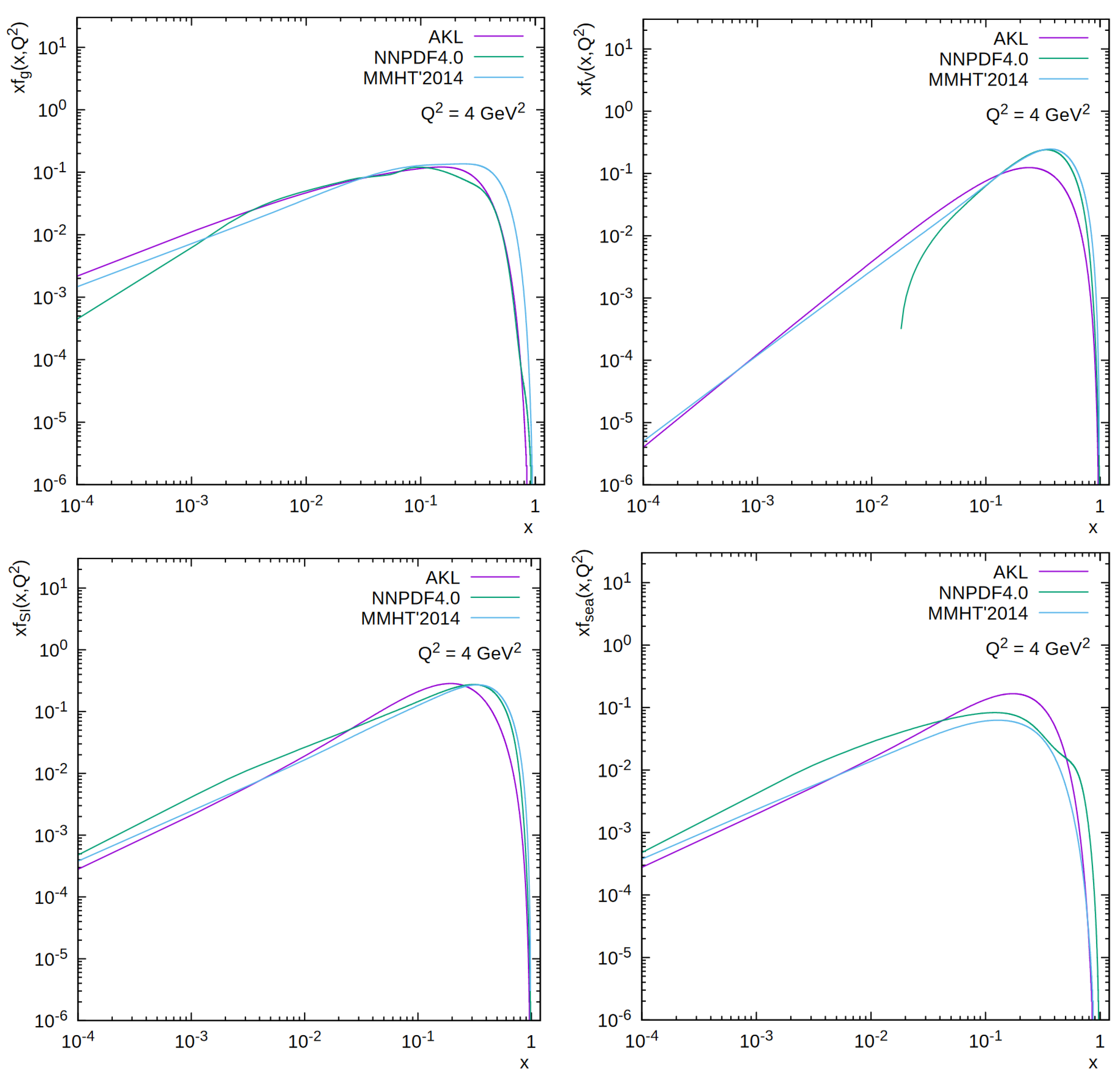
5.4. Results for Parton Densities

From numerical analysis we have B ( s ) = 0 , i.e., the large x behavior is defined by the valence quarks. Then, the results for f a , ( x , Q 2 ) with a = q or g in (57) are strongly simplified:
f q , ( x , Q 2 ) = A q e d s ( 1 x ) m q , + D ( s ) x ( 1 x ) ( 1 x ) ν ( s ) , f g , ( x , Q 2 ) = A g e d s ( 1 x ) ν ( s ) + m g , + 1 .
Similar simplification takes place also for f a , ( x , Q 0 2 ) in (74). To obtain it, we should take s = 0 in the results (75).
Moreover, we also have simplifications for G a ( s ) with a = q or g in (65), for G ¯ q ( s ) in (71) and for G a ( s = 0 ) in (73). Indeed, we should replace G a ( s ) in (65) by
G q ( s ) = A q 1 + ν ( s ) + m q , e d s + D ( s ) Γ ( 3 / 2 ) Γ ( 2 + ν ( s ) ) Γ ( 7 / 2 + ν ( s ) ) , G g ( s ) = A g ( ) 2 + ν ( s ) + m g , e d s .
and G a ( s = 0 ) ( a = q , g ) in (73) by the results (76) with s = 0 . The results G ¯ q ( s ) in (71) should be replaced by
G ¯ q ( s ) = A q 1 + ν ( s ) + m q , e d s .
The values of all the parameters involved in derived expressions can be determined from the comparison with known parametrizations of numerical solutions of the DGLAP equations and/or taking into account the sum rules. In our analysis, we employ the latest parametrizations proposed by the NNPDF Collaboration, namely, NNPDF4.0 set [7]. The results of our fit are collected in Table 1. Additionally, in Figure 1 we show a comparison between our PDFs (labeled as AKL) and corresponding results obtained by the MMHT’2014 [81] and NNPDF groups. We find good agreement between our analytical derivation and relevant numerical analyses.

6. TMD Parton Densities in the Proton

Now, we turn to the derivation of analytical expressions for the TMD gluon and quark density functions in the proton. Our consideration is based on the KMR procedure [32,33], which is a formalism to construct the TMDs from conventional PDFs. The key assumption is that the transverse momentum dependence of the parton distributions enters only at the last evolution step, so conventional PDFs can be used up to this step. There are known differential and integral formulations of the KMR approach in the literature (see [82,83,84] for more information and discussion). Below we derive expressions for the TMDs using both of these schemes.

6.1. Differential Formulation

In the differential formulation of the KMR procedure, we have the TMD parton densities f a ( d ) ( x , k 2 , Q 2 ) , where a = V , q or g as
f a ( d ) ( x , k 2 , Q 2 ) = ln k 2 T a ( Q 2 , k 2 ) D ^ a ( x , k 2 ) ,
where the Sudakov form factor T a ( Q 2 , k 2 ) has the following form:
T a ( Q 2 , k 2 ) = exp k 2 Q 2 d p 2 p 2 b = q , g 0 x 0 d z z P b a ( z , p 2 ) ,
with the splitting functions
P a b ( z , k 2 ) = 2 a s ( k 2 ) P a b ( LO ) ( z ) + ,
related with the LO anomalous dimensions (19) as
γ a b ( LO ) ( n ) = ) 2 d z z n 1 P a b ( LO ) ( z ) .
The PDFs D ^ a ( x , k 2 ) have the following form:
f a ( x , k 2 ) = x D ^ a ( x , k 2 ) .
Since
f a ( x , k 2 ) = ± f a , ± ( x , k 2 ) , a = q , g ,
we see that the f a ( d ) ( x , k 2 , Q 2 ) have similar form
f a ( d ) ( x , k 2 , Q 2 ) = ± f a , ± ( d ) ( x , k 2 , Q 2 ) .
Using the expressions (56)–(57) for PDFs f a ( x , k 2 ) , we obtain the the final results for TMDs (the complete results are shown in Appendix C):
f i ( d ) ( x , k 2 , Q 2 ) = β 0 a s ( k 2 ) T q ( Q 2 , k 2 ) × { d q R q ( Δ ) r V ln 1 1 x f i ( x , k 2 ) [ d V ( 1 λ V ) A V e d V ( 1 λ ) s 2 ( 1 x ) + p V + r V Ψ ( 1 + ν V ( s 2 ) ) B i ( s 2 ) x Γ ( 1 + ν V ( s 2 ) ) ] ( 1 x ) ν V ( s 2 ) } , ( i = V , N S ) , f g , + ( d ) ( x , k 2 , Q 2 ) = β 0 a s ( k 2 ) T g ( Q 2 , k 2 ) × { d g R g ( Δ ) r + ln 1 1 x f g , + ( x , k 2 ) [ d ^ + I ¯ 1 ( σ 2 ) + d ¯ + I ¯ 0 ( σ 2 ) A g + e d ¯ + s 2 ( 1 x ) m g + + p + + r + Ψ ( 1 + ν + ( s 2 ) ) B + ( s 2 ) x Γ ( 1 + ν + ( s 2 ) ) ] ( 1 x ) ν + ( s 2 ) } , f q , + ( d ) ( x , k 2 , Q 2 ) = β 0 a s ( k 2 ) T q ( Q 2 , k 2 ) × { d q R q ( Δ ) r + ln 1 1 x f q , + ( x , k 2 ) d ^ + I ¯ 0 ( σ 2 ) + d ¯ + I ˜ 1 ( σ 2 ) A q + e d ¯ + s 2 ( 1 x ) ν + ( s 2 ) + 1 + m q + } , f q , ( d ) ( x , k 2 , Q 2 ) = β 0 a s ( k 2 ) T q ( Q 2 , k 2 ) × { d q R q ( Δ ) r ln 1 1 x f q , ( x , k 2 ) d A q e d s 2 ( 1 x ) ν ( s 2 ) + m q } , f g , ( d ) ( x , k 2 , Q 2 ) = β 0 a s ( k 2 ) T g ( Q 2 , k 2 ) × { d g R g ( Δ ) r ln 1 1 x f g , ( x , k 2 ) d A g e d s 2 ( 1 x ) ν ( s 2 ) + m g + 1 } ,
where we neglected the derivations of D a ( s ) ( a = V , ± ) . Indeed, the magnitudes D a ( s ) of intermediate terms have slow s dependence and their derivations can be neglected.

6.2. Integral Formulation

Following the investigations performed in [30], we can obtain the following results ( j = V , N S ):
f j ( i ) ( x , k 2 , Q 2 ) = β 0 a s ( k 2 ) T q ( Q 2 , k 2 ) × { d q R q ( Δ ) r V ln 1 1 x f j ( x , k 2 ) R ˜ j ( x , k 2 ) } , f a ( i ) ( x , k 2 , Q 2 ) = f a , + ( i ) ( x , k 2 , Q 2 ) + f a , ( i ) ( x , k 2 , Q 2 ) , f a , ( i ) ( x , k 2 , Q 2 ) = β 0 a s ( k 2 ) T a ( Q 2 , k 2 ) × { d a R a ( Δ ) r ln 1 1 x f a , ( x , k 2 ) R ˜ a , ( x , k 2 ) } , f a , + ( i ) ( x , k 2 , Q 2 ) = β 0 a s ( k 2 ) T a ( Q 2 , k 2 ) × { d a R a ( Δ ) r + ln 1 1 x f ¯ a , + ( x , k 2 ) R ˜ a , + ( x , k 2 ) }
where
R ˜ j ( x , k 2 ) = d V ( 1 λ V ) A j e d V ( 1 λ ) s 2 x ¯ λ + p V + r V Ψ ( 1 + ν V ( s 2 ) ) B j ( s 2 ) x Γ ( 1 + ν V ( s 2 ) ) ( 1 x ) ν V ( s 2 ) + 1 , R ˜ q , + ( x , k 2 ) = d ^ + I ¯ 0 ( σ ¯ 2 ) + d ¯ + I ˜ 1 ( σ ¯ 2 ) A q + e d ¯ + s 2 ( 1 x ) ν + ( s 2 ) + m q , + + 2 , R ˜ g , + ( x , k 2 ) = [ d ^ + I ¯ 1 ( σ ¯ 2 ) + d ¯ + I ¯ 0 ( σ ¯ 2 ) A g + e d ¯ + s 2 ( 1 x ) m g , + + p + + r + Ψ ( 1 + ν V ( s 2 ) ) B + ( s 2 ) x Γ ( 1 + ν + ( s 2 ) ) ] ( 1 x ) ν + ( s 2 ) , R ˜ q , ( x , k 2 ) = d A q e d s 2 ( 1 x ) ν ( s 2 ) + m g , , R ˜ g , ( x , k 2 ) = d A g e d s 2 ( 1 x ) ν ( s 2 ) + m g , + 2 ,
with
x ¯ = x x 0 , x 0 = 1 Δ , σ ¯ 2 = σ 2 ( x x ¯ ) , ρ ¯ 2 = ρ 2 ( x x ¯ ) .
and
f ¯ a , + ( x , k 2 ) = f a , + ( x , k 2 ) w i t h σ 2 σ ¯ 2 , ρ 2 ρ ¯ 2 .
As in (85), we neglected contributions coming from the magnitudes D a ( s ) , where a = V , ±.

6.3. Sudakov form Factors T a ( Q 2 , k 2 )

For the Sudakov form factors, we have [31]:
T a ( Q 2 , k 2 ) = exp d a R a ( Δ ) s 1 ,
where
s 1 = ln a s ( k 2 ) a s ( Q 2 ) , d a = 4 C a β 0 , C q = C F , C g = C A , β 0 = C A 3 11 2 φ , R q ( Δ ) = ln 1 Δ 3 x 0 2 4 = ln 1 Δ 3 4 ( 1 Δ ) 2 , R g ( Δ ) = ln 1 Δ 1 φ 4 x 0 2 + 1 φ 12 x 0 3 ( 4 3 x 0 ) = = ln 1 Δ 1 φ 4 ( 1 Δ ) 2 + 1 φ 12 ( 1 Δ ) 3 ( 1 + 3 Δ ) .

6.4. Cut-Off Parameter Δ

For phenomenological applications, the cut-off parameter Δ usually has one of two basic forms:
Δ 1 = k Q , Δ 2 = k k + Q ,
that reflects two cases: Δ 1 is for the strong ordering, Δ 2 is for the angular ordering (see [82]). In all the cases above, except the results for T a ( Q 2 , k 2 ) , we can simply replace the parameter Δ by Δ 1 and/or Δ 2 . For the Sudakov form factors, we note that the parameters Δ i (with i = 1 , 2 ) contribute to the integrand and, thus, their momentum dependence changes the results in (90). Perfoming the correct evaluation (see [31]), we have
T a ( i ) ( Q 2 , k 2 ) = exp 4 C a k 2 Q 2 d p 2 p 2 a s ( p 2 ) R a ( Δ i ) .
Analytic evaluation of T a ( i ) ( Q 2 , k 2 ) is a very cumbersome procedure, which will be accomplished in the future. For the sake of simplifying our analysis, below we use numerical results for T a ( i ) ( Q 2 , k 2 ) .

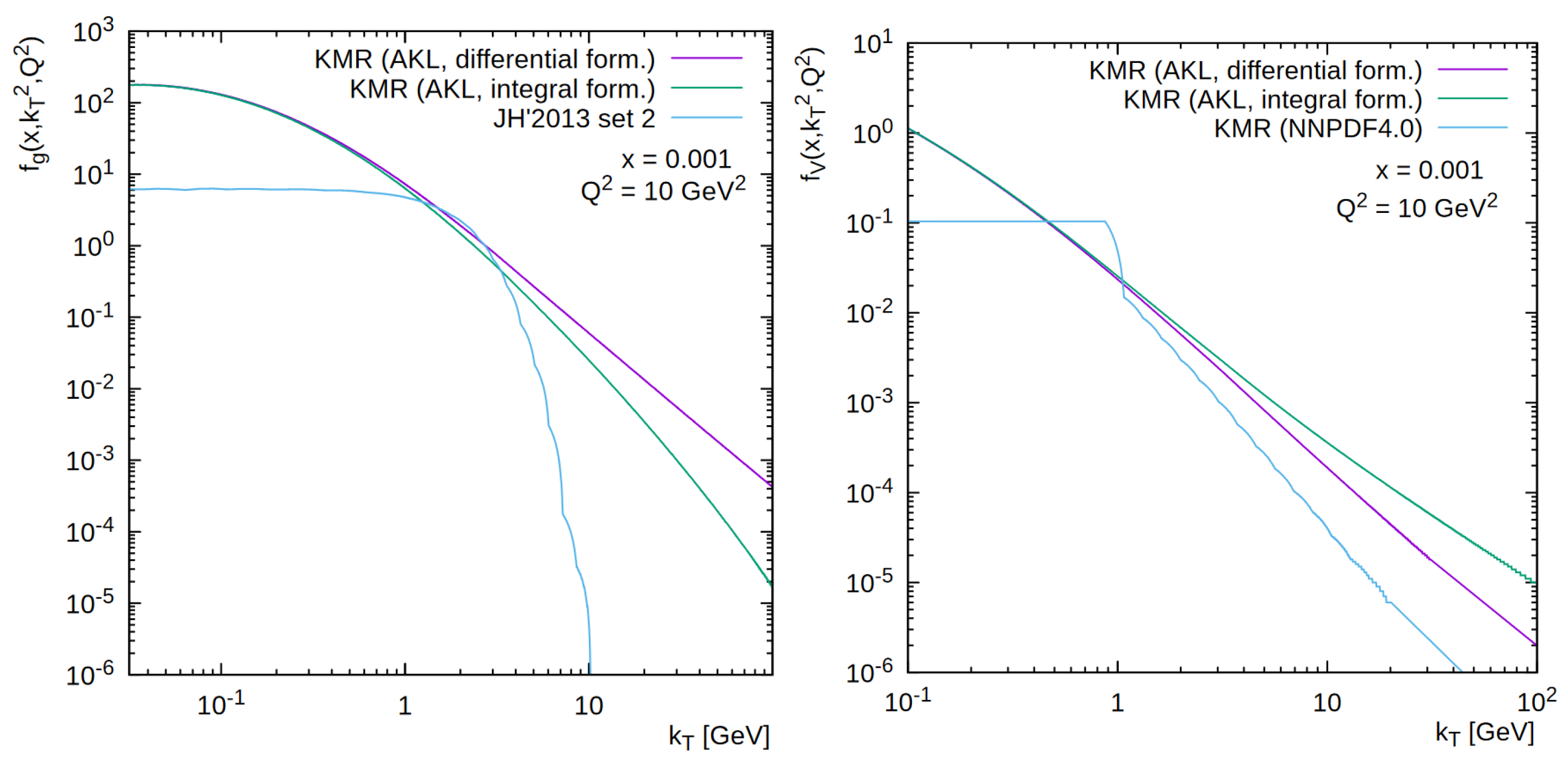
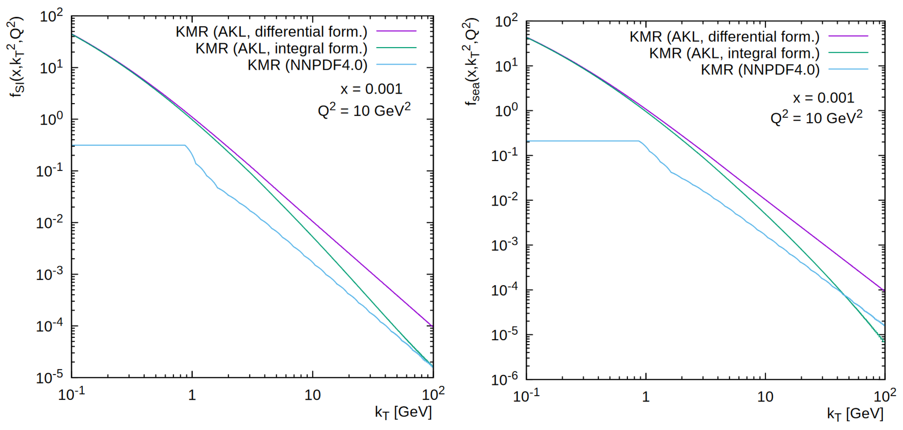
6.5. Results for TMD Parton Densities

Our results for the TMD quark and gluon densities in the proton, obtained in both differential and integral formulations of the KMR procedure, are shown in Figure 2. Note that the cut-off parameter Δ is taken in the form corresponding to the angular ordering condition. We find that the difference between these two scenarios originates at large parton transverse momenta only, whereas at low k T they match each other. In addition, we plot here for comparison results derived in other approaches. So, we show the TMD gluon distribution obtained from the numerical solution [85] of the Catani–Ciafaloni–Fiorani–Marchesini (CCFM) evolution equation [86,87,88,89], namely, JH’2013 set 2. The CCFM equation smoothly interpolates between the small-x BFKL gluon dynamics and large-x DGLAP one, and JH’2013 set 2 gluon is often used in different phenomenological applications (see, for example, [37,38,39,40]). Moreover, we plot here results for the TMD PDFs obtained within the KMR approach where the NNPDF4.0 set has been used as the input. One can see that all these TMDs have different shapes in k T and different overall normalization. The step behavior at low k T 1 GeV is related to a special normalization condition usually applied in the KMR scheme (see [32,33] for more information). Studying the phenomenological consequences of the observed differences is an important and interesting task, but it is out of our present consideration.

7. Conclusions

In the paper, we have proposed analytical expressions for the proton PDFs based on their exact asymptotics at small and large x values. The derived parameterizations contain subasymptotic terms, which are fixed by momentum conservation and, in the nonsinglet and valence parts, by the Gross–Llewellyn–Smith and Gottfried sum rules (see [28,29], respectively). The rest of the parameters are fixed by comparison with a recent numerical solution of the DGLAP equation performed by the NNPDF group [7] and presented in Table 1. Then, our consideration has been extended to the parton densities, dependent on the transverse momentum (TMDs). These quantities are often used in phenomenological applications and are widely discussed in the literature. We employ the popular Kimber–Martin–Ryskin formalism [32,33,34] and derive the TMD quark and gluon distributions in the proton within both differential and integral formulations of the KMR scheme. In the calculations, we have considered different treatments of kinematical constraint, reflecting the angular and strong ordering conditions. The analytical expressions for the PDFs and TMDs (in particular, for the quark TMDs), valid at both low and large x, have been obtained for the first time. As the next step, we plan to use the presented PDF sets to study PDF modifications in nuclei and, of course, to extend the present investigations beyond LO. In these investigations, we will follow [73,74,90,91,92,93,94,95,96], respectively.

Author Contributions

Investigation, N.A.A., A.V.K. and A.L.; Writing—original draft, N.A.A., A.V.K. and A.L. All authors have read and agreed to the published version of the manuscript.

Funding

Researches described in Section 3, Section 4 and Section 5 were supported by the Russian Science Foundation under grant 22-22-00387. Studies described and performed in Section 6 were supported by the Russian Science Foundation under grant 22-22-00119.

Data Availability Statement

Not applicable.

Acknowledgments

We thank M.A. Malyshev for very useful discussions and remarks.

Conflicts of Interest

The authors declare no conflict of interest.

Appendix A. PDF Asymptotics at Large x Values

Using large n expansion for S 1 ( n ) as
S 1 ( n ) = ln n + γ E + O ( n 1 ) ,
of some auxiliary anomalous dimension d c = c 1 S 1 ( n ) + c 2 , we see for the general renorm-group exponent
e d c s = e ( c 1 ( l n ( n ) + γ E ) c 2 ) s + O ( n 1 ) = n c 1 s e c ¯ 2 s + O ( n 1 ) , c ¯ 2 = c 2 + c 1 γ E .
Let some Mellin moment f c ( n , Q 2 ) of corresponding PDF f c ( x , Q 2 ) following (18), have the Q 2 -dependence
f c ( n , Q 2 ) = f c ( n , Q 0 2 ) e d c s = f c ( n , Q 0 2 ) n c 1 s e c ¯ 2 s .
It is convenient to represent our basic variable s shown in Equation (26) as
s = s ¯ ( Q 2 ) s ¯ ( Q 0 2 ) s ¯ s ¯ 0 ,
where
s ¯ ( Q 2 ) = ln [ ln ( Q 2 / Λ LO 2 ) ] .
Then we can see that the result (A3) for f c ( n , Q 2 ) can be rewritten as
f c ( n , Q 2 ) = B c n ν 1 c 1 s ¯ e ν 2 c ¯ 2 s ¯ ,
with some free parameters B c , ν 1 and ν 2 . For the initial condition f c ( x , Q 0 2 ) , we have the same result but with the replacement s s 0 .
Now we consider the Mellin moment
M c ( n ) = 0 1 d x x n 1 ( 1 x ) ν c = Γ ( n ) Γ ( ν c + 1 ) Γ ( n + ν c + 1 )
and try to represent it in a form, similar to (A3) and (A13).
It is convenient to use the Sterling formula
ln Γ ( z ) = z ln z z + 1 2 ln 2 π z + B 2 2 z + O ( z 2 )
at large z values, where B 2 is the Bernoulli number.
So, for large z and fixed δ values, we have after a little algebra
ln Γ ( z + δ ) Γ ( z ) = δ ln z + δ ( δ 1 ) 2 z + O ( z 2 )
and, thus,
Γ ( z ) Γ ( z + δ ) = z δ e δ ( 1 δ ) / ( 2 z ) + O ( z 2 ) = z δ 1 + δ ( 1 δ ) 2 z + O ( z 2 )
So, the Mellin moment M c ( n ) can be represented as
M c ( n ) = n ( ν c + 1 ) 1 ν c ( 1 + ν c ) 2 n + O ( n 2 )
For the PDF f c ( x , Q 2 ) we have ( ( α + 1 ) ν 1 + c 1 s ¯ )
f c ( x , Q 2 ) = B c ( 1 x ) ν c + c 1 s ¯ Γ ( ν c + 1 + c 1 s ¯ ) e ν 2 c ¯ 2 s ¯ = f c ( x , Q 0 2 ) Γ ( ν c + 1 + c 1 s ¯ 0 ) Γ ( ν c + 1 + c 1 s ¯ ) e c ¯ 2 s ,
where ν c = ν 1 1 . The constant ν 2 can be neglected.
So, finally we have
f c ( x , Q 2 ) = B ¯ c ( 1 x ) ν c ( s ) Γ ( ν c ( s ) + 1 ) e c ¯ 2 s , ν c ( s ) = ν c ( 0 ) + c ¯ 2 s ,
where
ν c ( 0 ) = ν c + c 1 s ¯ 0 , B ¯ c = f c ( x , Q 2 ) Γ ( ν c ( 0 ) + 1 ) ( 1 x ) ν c ( 0 ) e c ¯ 2 s ¯ 0

Appendix A.1. O(n0) Accuracy

At O ( n 0 ) accuracy,
γ q g = γ g q = O ( n 1 ) ,
and, thus, the Q 2 -evolutions of the singlet quark and gluon densities are not related to each other.
The corresponding anomalous dimesions have the following form
γ a = 8 C F ln n + γ E 3 4 + O ( n 1 ) , ( a = N S , V , q q ) , γ a = 8 C A ln n + γ E 2 β 0 + O ( n 1 ) ,
and parton densities
f q ( x , Q 2 ) = f ( x , Q 2 ) + O ( n 1 ) , f g ( x , Q 2 ) = f + ( x , Q 2 ) + O ( n 1 ) ,
have the large x asymptotics
f b ( x , Q 2 ) = B b ( s ) ( 1 x ) ν b ( s ) Γ ( ν b ( s ) + 1 ) , B b ( s ) = B b ( 0 ) e p b s , ν b ( s ) = ν b ( 0 ) + r b s , ( b = N S , V , ± )
where r b and p b are given in Equations (52).

Appendix A.2. O(n1) Accuracy

At O ( n 1 ) accuracy,
γ q g = 4 f n + O ( n 2 ) , γ g q = 4 C F n + O ( n 2 ) , γ q q = 8 C F ln n + c ^ + 1 2 n + O ( n 2 ) , γ g g = 8 C A ln n + c ^ + + 1 2 n + O ( n 2 ) .
where c ^ ± are given in Equation (53).
Using these results, we have
γ + = γ g g + O ( n 2 ) , γ = γ q q + O ( n 2 ) ,
i.e., the evolution of the “±”-components is the same as in the previous subsection.
The corresponding projectors have the following form:
α = 1 + O ( n 2 ) , β = K n 1 ln n + c ^ , ε ˜ = K + n 1 ln n + c ^ ,
where K ± and c ^ are given in Equation (53).
Thus, now the contributions of the initial quarks (gluons) to the final quarks (gluons) during Q 2 evolution are the same as in the previous subsection (see Equation (A18)) but there are additional contributions: initial quarks to gluons and vice versa. The last contributions have an unusual form ∼ 1 n ln n at large n values.
So, for the Q 2 -evolutions of the singlet quark and gluon densities we have
f a ( n , Q 2 ) = f ^ a + ( n , Q 0 2 ) e d + s + f ^ a ( n , Q 0 2 ) e d s ,
where
f ^ q + ( n , Q 0 2 ) = β f g ( n , Q 0 2 ) , f ^ q ( n , Q 0 2 ) = f q ( n , Q 0 2 ) + β f g + ( n , Q 0 2 ) , f ^ g ( n , Q 0 2 ) = ϵ f q ( n , Q 0 2 ) , f ^ g + ( n , Q 0 2 ) = f g ( n , Q 0 2 ) ϵ f q + ( n , Q 0 2 ) ,
Thus, the NS and valence parton densities have the large x asymptotics, shown in Equation (51) of the main text. For the singlet quark and gluon densities the situation is different. Their large x asymptotics contain standard contributions: the “+”-component for the gluon density and the “−”-component for the sea quark density (see Equation (A18), for example). However, there are also additional parts, ∼ K ± in Equation (51), coming from the contributions ∼ β and ∼ in (A23). We will sketch a way to calculate the additional parts f ¯ ± ( x , Q 2 ) in Appendix B.

Appendix B. Results at Large ν Values

To obtain the results f ¯ ± ( x , Q 2 ) it is convenient to calculate the inverse Mellin transform of the auxiliary function
f A ( n ) = 1 n ν + 2 ( ln n + a ) .
To do it, we expand the denominator of f A ( n ) as
f A ( n ) = 1 n ν + 2 ( ln n + a ) = m = 0 ( 1 ) m ln m n n ν + 2 a m + 1 = m = 0 1 a m + 1 d d ν m 1 n ν + 2
Since
0 1 d x x n 2 ( 1 x ) ν + 1 Γ ( ν + 2 ) ( n 1 ) ν + 1 Γ ( ν + 2 ) n ν + 1 ,
then the function f A ( x ) , which is the inverse Mellin transform of f A ( n )
f A ( n ) = 0 1 d x x n 2 f A ( x ) ,
has the form
f A ( x ) = m = 0 ( 1 ) m a m + 1 d d ν m ( 1 x ) ν + 1 Γ ( ν + 2 ) = m = 0 ( 1 ) m a m + 1 k = 0 m C k m d d ν m l ( 1 x ) ν + 1 d d ν l 1 Γ ( ν + 2 ) .
In the r.h.s. we will have powers of Polygamma functions
Ψ ( ν + 2 ) = d d ν ln Γ ( ν + 2 ) , Ψ ( m + 1 ) ( ν + 2 ) = d d ν Ψ ( m ) ( ν + 2 ) , ( m 0 ) .
At large ν -values, Ψ ( ν + 2 ) ln ( ν + 2 ) and Ψ ( m ) ( ν + 2 ) 1 / ( ν + 2 ) m , ( m 1 ) . So, we can neglect contributions from Ψ ( m ) ( ν + 2 ) , ( m 1 ) and obtain
d d ν l 1 Γ ( ν + 2 ) ( 1 ) l Ψ l ( ν + 2 ) Γ ( ν + 2 ) .
So, we have
f A ( x ) m = 0 ( 1 ) m a m + 1 ln 1 1 x + Ψ ( ν + 2 ) m ( 1 x ) ν + 1 Γ ( ν + 2 ) = 1 ln 1 1 x + a + Ψ ( ν + 2 ) ( 1 x ) ν + 1 Γ ( ν + 2 ) .
To obtain the contribution ∼ K in Equations (65) and (73), it is convenient to calculate the following auxiliary integral
I ( μ ) = 0 1 d x x μ f A ( x ) = 0 1 d x x μ ln 1 1 x + a + Ψ ( ν + 2 ) ( 1 x ) ν + 1 Γ ( ν + 2 ) .
Expanding the denominator as in Equation (A25), we have
I ( μ ) = m = 0 ( 1 ) m a m + 1 0 1 d x x μ ln 1 1 x + Ψ ( ν + 2 ) m ( 1 x ) ν + 1 Γ ( ν + 2 )
As it was shown above in Equations (A28) and (A31) the integral in the r.h.s. has the following form
0 1 d x x μ ln 1 1 x + Ψ ( ν + 2 ) m ( 1 x ) ν + 1 Γ ( ν + 2 ) ( 1 ) m d d ν m 0 1 d x x μ ( 1 x ) ν + 1 Γ ( ν + 2 ) = ( 1 ) m d d ν m Γ ( μ + 1 ) Γ ( μ + ν + 3 ) Ψ m ( μ + ν + 3 ) Γ ( μ + 1 ) Γ ( μ + ν + 3 ) .
So, for the auxiliary integral I ( μ ) we have
I ( μ ) m = 0 ( 1 ) m a m + 1 Ψ m ( μ + ν + 3 ) Γ ( μ + 1 ) Γ ( μ + ν + 3 ) = 1 a + Ψ ( μ + ν + 3 ) Γ ( μ + 1 ) Γ ( μ + ν + 3 )
Thus, the results ∼ K for G g ( s ) in Equation (65) and for G g ( s = 0 ) in Equation (73), can be obtained from (A35) for μ = 1 .
To obtain the results (72) it is convenient to consider the following auxiliary integral
Φ j ( μ , ν ) = 0 1 d x x μ ρ j I j ( σ ) ( 1 x ) ν .
Expanding Bessel function, we have
Φ j ( μ , ν ) = 0 1 d x x μ k = 0 ( d s ) k + j k ! ( k + j ) ! ln 1 x k ( 1 x ) ν .
As it was above in Equation (A34), the integral in the r.h.s. can be rewritten as
0 1 d x x μ ln 1 x k ( 1 x ) ν = ( 1 ) k d d μ k 0 1 d x x μ ( 1 x ) ν = ( 1 ) k d d μ k Γ ( μ + 1 ) Γ ( ν + 1 ) Γ ( μ + ν + 2 ) .
Taking approximations (A29), we have
0 1 d x x μ ln 1 x k ( 1 x ) ν = Ψ ( μ + ν + 2 ) Ψ ( μ + 1 ) k Γ ( μ + 1 ) Γ ( ν + 1 ) Γ ( μ + ν + 2 ) .
and, thus, the integral Φ j ( μ , ν ) is equal to
Φ j ( μ , ν ) = ρ μ j I j ( σ μ ) Γ ( μ + 1 ) Γ ( ν + 1 ) Γ ( μ + ν + 2 ) ,
where
σ μ = 2 d s ( Ψ ( μ + ν + 2 ) Ψ ( μ + 1 ) ) , ρ μ = σ μ 2 ( Ψ ( μ + ν + 2 ) Ψ ( μ + 1 ) ) .
The results (72) for Φ j ( ν ) ( j = 0 , 1 ) can be obtained from Equation (A36) at μ = 0 .

Appendix C. Differential Formulation of KMR Approach

Now we can find the results for TMD parton densities without derivatives. Derivation of T a ( Q 2 , k 2 ) is as follows
T a ( Q 2 , k 2 ) ln k 2 = d a β 0 a s ( k 2 ) R a ( Δ ) T a ( Q 2 , k 2 ) ,
and derivations of conventional PDFs are as follows
f V ( x , k 2 ) ln k 2 = β 0 a s ( k 2 ) { r V ln ( 1 x ) f V ( x , k 2 ) [ d V ( 1 λ V ) A V e d V ( 1 λ ) s 2 ( 1 x ) + p V + r V Ψ ( 1 + ν V ( s 2 ) ) B V ( s 2 ) x Γ ( 1 + ν V ( s 2 ) ) + D V * ( s 2 ) x ( 1 x ) ] ( 1 x ) ν V ( s 2 ) } , f g , + ( x , k 2 ) ln k 2 = β 0 a s ( k 2 ) { r + ln ( 1 x ) f g , + ( x , k 2 ) [ d ^ + I ¯ 1 ( σ 2 ) + d ¯ + I ¯ 0 ( σ 2 ) A g + e d ¯ + s 2 × ( 1 x ) m g + + p + + r + Ψ ( 1 + ν + ( s 2 ) ) B + ( s 2 ) x Γ ( 1 + ν + ( s 2 ) ) + D g + * ( s 2 ) x ( 1 x ) ] ( 1 x ) ν + ( s 2 ) } , f q , + ( x , k 2 ) ln k 2 = β 0 a s ( k 2 ) { r + ln ( 1 x ) f q , + ( x , k 2 ) d ^ + I ¯ 0 ( σ 2 ) + d ¯ + I ˜ 1 ( σ 2 ) A q + e d ¯ + s 2 ( 1 x ) ν + ( s 2 ) + 1 + m q + } , f q , ( x , k 2 ) ln k 2 = β 0 a s ( k 2 ) { r ln ( 1 x ) f q , ( x , k 2 ) [ d A q e d s 2 ( 1 x ) m q + D q * ( s 2 ) x ( 1 x ) ] ( 1 x ) ν ( s 2 ) } , f g , ( x , k 2 ) ln k 2 = β 0 a s ( k 2 ) r ln ( 1 x ) f g , ( x , k 2 ) d A g e d s 2 ( 1 x ) ν ( s 2 ) + m g + 1 ,
where
D * ( s ) = d d s D ( s ) , s 2 = ln a s ( Q 0 2 ) a s ( k 2 ) , σ 2 = σ ( s s 2 ) , ρ 2 = ρ ( s s 2 ) .
So, the results for the TMD parton densities read the form (84) with
f V ( d ) ( x , k 2 , Q 2 ) = β 0 a s ( k 2 ) T q ( Q 2 , k 2 ) × { d q R q ( Δ ) r V ln 1 1 x f V ( x , k 2 ) [ d V ( 1 λ V ) A V e d V ( 1 λ ) s 2 ( 1 x ) + p V + r V Ψ ( 1 + ν V ( s 2 ) ) B V ( s 2 ) x Γ ( 1 + ν V ( s 2 ) ) + D v * ( s 2 ) x ( 1 x ) ] ( 1 x ) ν V ( s 2 ) } , f g , + ( d ) ( x , k 2 , Q 2 ) = β 0 a s ( k 2 ) T g ( Q 2 , k 2 ) × { d g R g ( Δ ) r + ln 1 1 x f g , + ( x , k 2 ) [ d ^ + I ¯ 1 ( σ 2 ) + d ¯ + I ¯ 0 ( σ 2 ) A g + e d ¯ + s 2 ( 1 x ) m g + + p + + r + Ψ ( 1 + ν + ( s 2 ) ) B + ( s 2 ) x Γ ( 1 + ν + ( s 2 ) ) + D g + * ( s 2 ) x ( 1 x ) ] ( 1 x ) ν + ( s 2 ) } , f q , + ( d ) ( x , k 2 , Q 2 ) = β 0 a s ( k 2 ) T q ( Q 2 , k 2 ) × { d q R q ( Δ ) r + ln 1 1 x f q , + ( x , k 2 ) d ^ + I ¯ 0 ( σ 2 ) + d ¯ + I ˜ 1 ( σ 2 ) A q + e d ¯ + s 2 ( 1 x ) ν + ( s 2 ) + 1 + m q + } , f q , ( d ) ( x , k 2 , Q 2 ) = β 0 a s ( k 2 ) T q ( Q 2 , k 2 ) × { d q R q ( Δ ) r ln 1 1 x f q , ( x , k 2 ) d A q e d s 2 ( 1 x ) m q + D q * ( s 2 ) x ( 1 x ) ( 1 x ) ν ( s 2 ) } , f g , ( d ) ( x , k 2 , Q 2 ) = β 0 a s ( k 2 ) T g ( Q 2 , k 2 ) × { d g R g ( Δ ) r ln 1 1 x f g , ( x , k 2 ) d A g e d s 2 ( 1 x ) ν ( s 2 ) + m g + 1 } .

References

  1. Gribov, V.N.; Lipatov, L.N. Deep inelastic e p scattering in perturbation theory. Sov. J. Nucl. Phys. 1972, 15, 438. [Google Scholar]
  2. Lipatov, L.N. The parton model and perturbation theory. Sov. J. Nucl. Phys. 1975, 20, 94. [Google Scholar]
  3. Altarelli, G.; Parisi, G. Asymptotic Freedom in Parton Language. Nucl. Phys. 1977, 126, 298. [Google Scholar] [CrossRef]
  4. Dokshitzer, Y.L. Calculation of the Structure Functions for Deep Inelastic Scattering and e+ e- Annihilation by Perturbation Theory in Quantum Chromodynamics. Sov. Phys. JETP 1977, 46, 641. [Google Scholar]
  5. Hou, T.J.; Gao, J.; Hobbs, T.J.; Xie, K.; Dulat, S.; Guzzi, M.; Huston, J.; Nadolsky, P.; Pumplin, J.; Schmidt, C.; et al. New CTEQ global analysis of quantum chromodynamics with high-precision data from the LHC. Phys. Rev. D 2021, 103, 014013. [Google Scholar] [CrossRef]
  6. Bailey, S.; Cridge, T.; Harland-Lang, L.A.; Martin, A.D.; Thorne, R.S. Parton distributions from LHC, HERA, Tevatron and fixed target data: MSHT20 PDFs. Eur. Phys. J. C 2021, 81, 341. [Google Scholar] [CrossRef]
  7. NNPDF Collaboration; Ball, R.D.; Carrazza, S.; Cruz-Martinez, J.; Del Debbio, L.; Forte, S.; Giani, T.; Iranipour, S.; Kassabov, Z.; Latorre, J.I.; et al. An open-source machine learning framework for global analyses of parton distributions. Eur. Phys. J. C 2021, 81, 958. [Google Scholar]
  8. Abt, I.; Aggarwal, R.; Andreev, V.; Arratia, M.; Aushev, V.; Baghdasaryan, A.; Baty, A.; Begzsuren, K.; Behnke, O.; Belousov, A.; et al. Impact of jet-production data on the next-to-next-to-leading-order determination of HERAPDF2.0 parton distributions. Eur. Phys. J. C 2022, 82, 243. [Google Scholar] [CrossRef]
  9. Alekhin, S.; Blümlein, J.; Moch, S.; Placakyte, R. Parton distribution functions, αs, and heavy-quark masses for LHC Run II. Phys. Rev. D 2017, 96, 014011. [Google Scholar] [CrossRef] [Green Version]
  10. Jimenez-Delgado, P.; Reya, E. Delineating parton distributions and the strong coupling. Phys. Rev. D 2014, 89, 074049. [Google Scholar] [CrossRef] [Green Version]
  11. Parente, G.; Kotikov, A.V.; Krivokhizhin, V.G. Analysis of deep inelastic structure functions in perturbative QCD at three loops. Phys. Lett. 1994, 333, 190. [Google Scholar] [CrossRef] [Green Version]
  12. Kataev, A.L.; Kotikov, A.V.; Parente, G.; Sidorov, A.V. Next-to-next-to-leading order QCD analysis of the CCFR data xF3 and F2 structure functions of the deep-inelastic neutrino-nucleon scattering. Phys. Lett. 1996, 388, 179. [Google Scholar] [CrossRef] [Green Version]
  13. Kataev, A.L.; Kotikov, A.V.; Parente, G.; Sidorov, A.V. Next-to-next-to-leading order QCD analysis of the revised CCFR data for xF3 structure function and the higher twist contributions. Phys. Lett. 1998, 417, 374. [Google Scholar] [CrossRef] [Green Version]
  14. Sidorov, A.V. QCD analysis of the CCFR data for x F(3) and higher twist contribution. Phys. Lett. 1996, 389, 379. [Google Scholar]
  15. Kataev, A.L.; Parente, G.; Sidorov, A.V. Higher twists and alpha(s)(M(Z)) extractions from the NNLO QCD analysis of the CCFR data for the xF(3) structure function. Nucl. Phys. 2000, 573, 405. [Google Scholar] [CrossRef]
  16. Kataev, A.L.; Parente, G.; Sidorov, A.V. Improved fits to the xF3 CCFR data at the next-to-next-to-leading order and beyond. Phys. Part. Nucl. 2003, 34, 20. [Google Scholar] [CrossRef] [Green Version]
  17. Shaikhatdenov, B.G.; Kotikov, A.V.; Krivokhizhin, V.G.; Parente, G. QCD coupling constant at NNLO from DIS data. Phys. Rev. D 2010, 81, 034008. [Google Scholar] [CrossRef]
  18. Kotikov, A.V.; Krivokhizhin, V.G.; Shaikhatdenov, B.G. Strong coupling constant from QCD analysis of the fixed-target DIS data. JETP Lett. 2015, 101, 141–145. [Google Scholar] [CrossRef]
  19. Kotikov, A.V.; Krivokhizhin, V.G.; Shaikhatdenov, B.G. Improved nonsinglet QCD analysis of fixed-target DIS data. J. Phys. G 2015, 42, 095004. [Google Scholar] [CrossRef] [Green Version]
  20. Kotikov, A.V.; Krivokhizhin, V.G.; Shaikhatdenov, B.G. Analytic and ’frozen’ QCD coupling constants up to NNLO from DIS data. Phys. Atom. Nucl. 2012, 75, 507–524. [Google Scholar] [CrossRef] [Green Version]
  21. Kotikov, A.V.; Krivokhizhin, V.G.; Shaikhatdenov, B.G. Gottfried sum rule in QCD NS analysis of DIS fixed target data. Phys. Atom. Nucl. 2018, 81, 244–252. [Google Scholar] [CrossRef]
  22. Krivokhizhin, V.G.; Kotikov, A.V. A systematic study of QCD coupling constant from deep-inelastic measurements. Phys. Atom. Nucl. 2005, 68, 1873–1903. [Google Scholar] [CrossRef]
  23. Demartin, F.; Forte, S.; Mariani, E.; Rojo, J.; Vicini, A. The impact of PDF and alphas uncertainties on Higgs Production in gluon fusion at hadron colliders. Phys. Rev. D 2010, 82, 014002. [Google Scholar] [CrossRef] [Green Version]
  24. Illarionov, A.Y.; Kotikov, A.V.; Parzycki, S.S.; Peshekhonov, D.V. New type of parametrizations for parton distributions. Phys. Rev. D 2011, 83, 034014. [Google Scholar] [CrossRef] [Green Version]
  25. Lopez, C.; Yndurain, F.J. Behavior of Deep Inelastic Structure Functions Near Physical Region Endpoints From QCD. Nucl. Phys. B 1980, 171, 231. [Google Scholar] [CrossRef]
  26. Lopez, C.; Yndurain, F.J. Behavior at x = 0, 1, Sum Rules and Parametrizations for Structure Functions Beyond the Leading Order. Nucl. Phys. B 1981, 183, 157. [Google Scholar] [CrossRef] [Green Version]
  27. Yndurain, F.J. Quantum Chromodynamics (An Introduction to the Theory of Quarks and Gluons); Springer: Berlin/Heidelberg, Germany, 1983. [Google Scholar]
  28. Gross, D.J.; Smith, C.H.L. High-energy neutrino—Nucleon scattering, current algebra and partons. Nucl. Phys. B 1969, 14, 337. [Google Scholar] [CrossRef] [Green Version]
  29. Gottfried, K. Sum rule for high-energy electron—Proton scattering. Phys. Rev. Lett. 1967, 18, 1174. [Google Scholar] [CrossRef]
  30. Kotikov, A.V.; Lipatov, A.V.; Shaikhatdenov, B.G.; Zhang, P. Transverse momentum dependent parton densities in a proton from the generalized DAS approach. JHEP 2020, 28. [Google Scholar] [CrossRef] [Green Version]
  31. Kotikov, A.V.; Lipatov, A.V.; Zhang, P.M. Transverse momentum dependent parton densities in processes with heavy quark generations. Phys. Rev. D 2021, 104, 054042. [Google Scholar] [CrossRef]
  32. Kimber, M.A.; Martin, A.D.; Ryskin, M.G. Unintegrated parton distributions. Phys. Rev. D 2001, 63, 114027. [Google Scholar] [CrossRef] [Green Version]
  33. Watt, G.; Martin, A.D.; Ryskin, M.G. Unintegrated parton distributions and inclusive jet production at HERA. Eur. Phys. J. C 2003, 31, 73. [Google Scholar] [CrossRef] [Green Version]
  34. Martin, A.D.; Ryskin, M.G.; Watt, G. NLO prescription for unintegrated parton distributions. Eur. Phys. J. C 2010, 66, 163. [Google Scholar] [CrossRef]
  35. Angeles-Martinez, R.; Bacchetta, A.; Balitsky, I.I.; Boer, D.; Boglione, M.; Boussarie, R.; Ceccopieri, F.A.; Cherednikov, I.O.; Connor, P.; Echevarria, M.G.; et al. Transverse momentum dependent (TMD) parton distribution functions: Status and prospects. Acta Phys. Polon. B 2015, 46, 2501. [Google Scholar] [CrossRef]
  36. Sherstnev, A.; Thorne, R.S. Parton Distributions for LO Generators. Eur. Phys. J. 2008, 55, 553–575. [Google Scholar] [CrossRef]
  37. Maciula, R.; Pasechnik, R.; Szczurek, A. Production of forward heavy-flavor dijets at the LHCb within the kT-factorization approach. Phys. Rev. D 2022, 106, 054018. [Google Scholar] [CrossRef]
  38. Baranov, S.P.; Lipatov, A.V.; Prokhorov, A.A. Role of initial gluon emission in double J/Ψ production at central rapidities. Phys. Rev. D 2022, 106, 034020. [Google Scholar] [CrossRef]
  39. Abdulov, N.A.; Jung, H.; Lipatov, A.V.; Lykasov, G.I.; Malyshev, M.A. Employing RHIC and LHC data to determine the transverse momentum dependent gluon density in a proton. Phys. Rev. D 2018, 98, 054010. [Google Scholar] [CrossRef] [Green Version]
  40. Abdulov, N.A.; Lipatov, A.V.; Malyshev, M.A. Inclusive Higgs boson production at the LHC in the kt-factorization approach. Phys. Rev. D 2018, 97, 054017. [Google Scholar] [CrossRef] [Green Version]
  41. Ahrens, V.; Ferroglia, A.; Neubert, M.; Pecjak, B.D.; Yang, L.L. Renormalization-Group Improved Predictions for Top-Quark Pair Production at Hadron Colliders. JHEP 2010, 97. [Google Scholar] [CrossRef] [Green Version]
  42. Buras, A. Asymptotic Freedom in Deep Inelastic Processes in the Leading Order and Beyond. Rev. Mod. Phys. 1980, 52, 199. [Google Scholar] [CrossRef]
  43. Kotikov, A.V. Deep inelastic scattering: Q**2 dependence of structure functions. Phys. Part. Nucl. 2007, 38, 1, Erratum in Phys. Part. Nucl. 2007, 38, 828. [Google Scholar] [CrossRef]
  44. Krivokhizhin, V.G.; Kotikov, A.V. Functions of the nucleon structure and determination of the strong coupling constant. Phys. Part. Nucl. 2009, 40, 1059. [Google Scholar] [CrossRef]
  45. Kotikov, A. Parton distributions at low x and gluon- and quark average multiplicities. arXiv 2015, arXiv:1502.07108. [Google Scholar]
  46. Arneodo, M.; Arvidson, A.; Badelek, B.; Ballintijn, M.; Baum, G.; Beaufays, J.; Bird, I.G.; Bjorkholm, P.; Botje, M.; Broggini, C.; et al. A Reevaluation of the Gottfried sum. Phys. Rev. D 1994, 50, R1–R3. [Google Scholar] [CrossRef] [Green Version]
  47. Kotikov, A.V.; Velizhanin, V.N. Analytic continuation of the Mellin moments of deep inelastic structure functions. arXiv 2005, arXiv:hep-ph/0501274. [Google Scholar]
  48. Kazakov, D.I.; Kotikov, A.V. Total αs correction to the ratio of the deep inelastic scattering cross-sections R=σL/σT in QCD. Nucl. Phys. 1988, 307, 791, Erratum in Nucl. Phys. 1990, 345, 299. [Google Scholar] [CrossRef]
  49. Kotikov, A.V. The extraction of gluon distribution from DIS structure funstions. Phys. Atom. Nucl. 1994, 57, 133. [Google Scholar]
  50. Gross, D.I. How to Test Scaling in Asymptotically Free Theories. Phys. Rev. Lett. 1974, 32, 1071. [Google Scholar] [CrossRef]
  51. Gross, D.I.; Treiman, S.B. Hadronic Form-Factors in Asymptotically Free Field Theories. Phys. Rev. Lett. 1974, 32, 1145. [Google Scholar] [CrossRef] [Green Version]
  52. Ball, R.D.; Forte, S. Double asymptotic scaling at HERA. Phys. Lett. B 1994, 335, 77. [Google Scholar] [CrossRef] [Green Version]
  53. De Rújula, A.; Glashow, S.L.; Politzer, H.D.; Treiman, S.B.; Wilczek, F.; Zee, A. Possible NonRegge Behavior of Electroproduction Structure Functions. Phys. Rev. D 1974, 10, 1649. [Google Scholar] [CrossRef] [Green Version]
  54. Mankiewicz, L.; Saalfeld, A.; Weigl, T. On the analytical approximation to the GLAP evolution at small x and moderate Q**2. Phys. Lett. B 1997, 393, 175. [Google Scholar] [CrossRef] [Green Version]
  55. Kotikov, A.V.; Parente, G. Small x behaviour of parton distributions with soft initial conditions. Nucl. Phys. B 1999, 549, 242. [Google Scholar] [CrossRef] [Green Version]
  56. Illarionov, A.Y.; Kotikov, A.V.; Parente, G. Small x behavior of parton distributions. A study of higher twist. Phys. Part. Nucl. 2008, 39, 307. [Google Scholar] [CrossRef] [Green Version]
  57. Kotikov, A.V.; Shaikhatdenov, B.G. Q2-evolution of parton densities at small x values. Phys. Part. Nucl. 2017, 48, 829. [Google Scholar] [CrossRef] [Green Version]
  58. Kotikov, A.V.; Shaikhatdenov, B.G. Q2-evolution of parton densities at small x values. Effective scale for combined H1 and ZEUS F2 data. Phys. Atom. Nucl. 2015, 78, 525. [Google Scholar] [CrossRef]
  59. Kotikov, A.V.; Shaikhatdenov, B.G. Q2-evolution of parton densities at small x values. Combined H1 and ZEUS F2 data. Phys. Part. Nucl. 2013, 44, 543. [Google Scholar] [CrossRef]
  60. Kotikov, A.V.; Shaikhatdenov, B.G. Q2-evolution of parton densities at small x values and H1 and ZEUS experimental data. AIP Conf. Proc. 2015, 1606, 159–167. [Google Scholar]
  61. Cvetic, G.; Illarionov, A.Y.; Kniehl, B.A.; Kotikov, A.V. Small-x behavior of the structure function F(2) and its slope lnF(2)/ln(1/x) for ’frozen’ and analytic strong-coupling constants. Phys. Lett. B 2009, 679, 350. [Google Scholar] [CrossRef] [Green Version]
  62. Illarionov, A.Y.; Kotikov, A.V. F 2 c at low x. Phys. Atom. Nucl. 2012, 75, 1234–1239. [Google Scholar] [CrossRef]
  63. Kotikov, A.V. Gluon distribution as function of F2 and dF2/dlnQ**2 at small x. JETP Lett. 1994, 59, 667–670. [Google Scholar]
  64. Kotikov, A.V.; Parente, G. The Gluon distribution as a function of f2 and dF2 - dlnQ**2 small x. The Next-to-leading analysis. Phys. Lett. B 1996, 379, 195–201. [Google Scholar] [CrossRef] [Green Version]
  65. Kotikov, A.V. Longitudinal structure function F(L) as function of F2 and dF2/dlnQ**2 at small x. J. Exp. Theor. Phys. 1995, 80, 979–982. [Google Scholar]
  66. Kotikov, A.V.; Parente, G. The Longitudinal structure function FL as a function of F2 and dF2/dlnQ**2 at small x. The Next-to-leading analysis. Mod. Phys. Lett. A 1997, 12, 963–974. [Google Scholar] [CrossRef] [Green Version]
  67. Kotikov, A.V.; Parente, G. Indirect determination of the ratio R = Sigma(L)/Sigma(T) at small x from HERA data. J. Exp. Theor. Phys. 1997, 85, 17–19. [Google Scholar] [CrossRef]
  68. Illarionov, A.Y.; Kniehl, B.A.; Kotikov, A.V. Heavy-quark contributions to the ratio F(L)/F(2) at low x. Phys. Lett. B 2008, 663, 66–72. [Google Scholar] [CrossRef] [Green Version]
  69. Kotikov, A.V. On the behavior of DIS structure function ratio R (x, Q**2) at small x. Phys. Lett. B 1994, 338, 349–356. [Google Scholar] [CrossRef]
  70. Kotikov, A.V. Gluon distribution as function of F(L) and F(2) at small x. Phys. Rev. D 1994, 49, 5746–5752. [Google Scholar] [CrossRef]
  71. Kotikov, A.V.; Parente, G. QCD relations between structure functions at small x. arXiv 1997, arXiv:hep-ph/9710252. [Google Scholar]
  72. Kotikov, A.V.; Parente, G. Small x behavior of the slope dlnF(2)/dln(1/x) in the framework of perturbative QCD. J. Exp. Theor. Phys. 2003, 97, 859–867. [Google Scholar] [CrossRef] [Green Version]
  73. Kotikov, A.V.; Shaikhatdenov, B.G.; Zhang, P. Application of the rescaling model at small Bjorken x values. Phys. Rev. D 2017, 96, 114002. [Google Scholar] [CrossRef]
  74. Kotikov, A.V.; Shaikhatdenov, B.G.; Zhang, P. Antishadowing in the rescaling model at x∼0.1. Phys. Part. Nucl. Lett. 2019, 16, 311. [Google Scholar] [CrossRef] [Green Version]
  75. Matveev, V.A.; Muradian, R.M.; Tavkhelidze, A.N. Automodellism in the large—Angle elastic scattering and structure of hadrons. Lett. Nuovo Cim. 1973, 7, 719. [Google Scholar] [CrossRef]
  76. Brodsky, S.J.; Farrar, G.R. Scaling Laws at Large Transverse Momentum. Phys. Rev. Lett. 1973, 31, 1153. [Google Scholar] [CrossRef] [Green Version]
  77. Brodsky, S.J.; Ellis, J.; Cardi, E.; Karliner, M.; Samuel, M.A. Pade approximants, optimal renormalization scales, and momentum flow in Feynman diagrams. Phys. Rev. 1997, 56, 6980. [Google Scholar] [CrossRef] [Green Version]
  78. Kotikov, A.V. THE BEHAVIOR OF THE STRUCTURE FUNCTIONS AND RATIO R = sigma-L/sigma-T IN DEEP INELASTIC SCATTERING FOR x approximates 0 AND x approximates 1 AND THEIR SCHEME INVARIANT PARAMETRIZATION. JINR Preprint: JINR-E2-88-422. 1988. Available online: https://inspirehep.net/literature/265682 (accessed on 30 October 2022).
  79. Kotikov, A.V.; Maksimov, S.I.; Vovk, V.I. QCD parameterization for structure functions of deep inelastic scattering. Theor. Math. Phys. 1991, 84, 744. [Google Scholar]
  80. Kotikov, A.V.; Maximov, S.I.; Parobij, I.S. QCD parameterization of the parton distributions of deep inelastic scattering. Theor. Math. Phys. 1997, 111, 442. [Google Scholar] [CrossRef]
  81. Harland-Lang, L.A.; Martin, A.D.; Motylinski, P.; Thorne, R.S. Parton distributions in the LHC era: MMHT 2014 PDFs. Eur. Phys. J. C 2015, 75, 204. [Google Scholar] [CrossRef] [Green Version]
  82. Golec-Biernat, K.; Stasto, A.M. On the use of the KMR unintegrated parton distribution functions. Phys. Lett. B 2018, 781, 633. [Google Scholar] [CrossRef]
  83. Guiot, B. Pathologies of the Kimber-Martin-Ryskin prescriptions for unintegrated PDFs: Which prescription should be preferred? Phys. Rev. D 2020, 101, 054006. [Google Scholar] [CrossRef] [Green Version]
  84. Valeshabadi, R.K.; Modarres, M. On the ambiguity between differential and integral forms of the Martin–Ryskin–Watt unintegrated parton distribution function model. Eur. Phys. J. C 2022, 82, 66. [Google Scholar] [CrossRef]
  85. Hautmann, F.; Jung, H. Transverse momentum dependent gluon density from DIS precision data. Nucl. Phys. B 2014, 883, 1. [Google Scholar] [CrossRef]
  86. Ciafaloni, M. Coherence Effects in Initial Jets at Small q**2/s. Nucl. Phys. B 1988, 296, 49. [Google Scholar] [CrossRef] [Green Version]
  87. Catani, S.; Fiorani, F.; Marchesini, G. QCD Coherence in Initial State Radiation. Phys. Lett. B 1990, 234, 339. [Google Scholar] [CrossRef]
  88. Catani, S.; Fiorani, F.; Marchesini, G. Small x Behavior of Initial State Radiation in Perturbative QCD. Nucl. Phys. B 1990, 336, 18. [Google Scholar] [CrossRef]
  89. Marchesini, G. QCD coherence in the structure function and associated distributions at small x. Nucl. Phys. B 1995, 445, 49. [Google Scholar] [CrossRef] [Green Version]
  90. Kotikov, A.V. THE EMC RATIO AS A FUNCTION OF x, Q**2 IN THE RESCALING MODEL. Sov. J. Nucl. Phys. 1989, 50, 127–128. [Google Scholar]
  91. Kotikov, A.V.; Lipatov, A.V.; Parente, G.; Zotov, N.P. The Contribution of off-shell gluons to the structure functions F(2)**c and F(L)**c and the unintegrated gluon distributions. Eur. Phys. J. C 2002, 26, 51. [Google Scholar] [CrossRef]
  92. Kotikov, A.V.; Lipatov, A.V.; Zotov, N.P. The Contribution of off-shell gluons to the longitudinal structure function F(L). Eur. Phys. J. C 2003, 27, 219. [Google Scholar] [CrossRef] [Green Version]
  93. Kotikov, A.V.; Lipatov, A.V.; Zotov, N.P. The Longitudinal structure function F(L): Perturbative QCD and k(T) factorization versus experimental data at fixed W. J. Exp. Theor. Phys. 2005, 101, 811–816. [Google Scholar] [CrossRef] [Green Version]
  94. van Hameren, A. A note on QED gauge invariance of off-shell amplitudes. arXiv 2019, arXiv:1902.01791. [Google Scholar]
  95. Nefedov, M.; Saleev, V. On the one-loop calculations with Reggeized quarks. Mod. Phys. Lett. A 2017, 32, 1750207. [Google Scholar] [CrossRef]
  96. Caporale, F.; Celiberto, F.G.; Chachamis, G.; Gordo Gomez, D.; Sabio Vera, A. Inclusive three- and four-jet production in multi-Regge kinematics at the LHC. AIP Conf. Proc. 2017, 1819, 060009. [Google Scholar]
Figure 1. The gluon, valence, singlet and sea quarks densities in the proton calculated as a function of the longitudinal momentum fraction x at hard scale Q 2 = 4 GeV 2 . The purple curve corresponds to the results obtained with AKL, the green and blue curves with NNPDF4.0 (LO) and MMHT’2014 (LO) parton density functions, respectively.
Particles 05 00039 g001
Figure 2. The TMD gluon, valence, singlet and sea quarks densities in the proton calculated as a function of the parton transverse momentum k T 2 at longitudinal momentum fraction x = 0.001 and hard scale Q 2 = 10 GeV 2 . The purple and green curves correspond to the results obtained with AKL sets, which were obtained from differential and integral formulations of KMR approach, respectively. The blue curve corresponds to the results obtained with TMD gluon distribution JH’2013 set 2 and with TMD quark distributions calculated numerically in the traditional KMR scenario, where the conventional parton densities from standard NNPDF (LO) set are used as an input.
Particles 05 00039 g002aParticles 05 00039 g002b
Table 1. The fitted values of various parameters involved in our analytical expressions for PDFs in the proton.
Q 0 , GeV A V ( 0 ) A q A g B V ( 0 ) B ( 0 ) B + ( 0 )
AKL 0.43 3.0 0.95 0.77 100.0 0.0 13 × 10 6
m q , m q , + m g , m g , + ν V ( 0 ) ν ( 0 ) ν + ( 0 )
AKL 2.0 1.0 1.0 2.0 4.0 7.2 8.2
Publisher’s Note: MDPI stays neutral with regard to jurisdictional claims in published maps and institutional affiliations.

