A Brief Introduction to Nonlinear Time Series Analysis and Recurrence Plots


Potsdam Institute for Climate Impact Research, Transdisciplinary Concepts & Methods, 14412 Potsdam, Germany
Vibration 2019, 2(4), 332-368; https://doi.org/10.3390/vibration2040021
Submission received: 21 February 2019
/
Revised: 29 November 2019
/
Accepted: 2 December 2019
/
Published: 8 December 2019
(This article belongs to the Special Issue Irregular Engineering Oscillations and Signal Processing)
Abstract
:Nonlinear time series analysis gained prominence from the late 1980s on, primarily because of its ability to characterize, analyze, and predict nontrivial features in data sets that stem from a wide range of fields such as finance, music, human physiology, cognitive science, astrophysics, climate, and engineering. More recently, recurrence plots, initially proposed as a visual tool for the analysis of complex systems, have proven to be a powerful framework to quantify and reveal nontrivial dynamical features in time series data. This tutorial review provides a brief introduction to the fundamentals of nonlinear time series analysis, before discussing in greater detail a few (out of the many existing) approaches of recurrence plot-based analysis of time series. In particular, it focusses on recurrence plot-based measures which characterize dynamical features such as determinism, synchronization, and regime changes. The concept of surrogate-based hypothesis testing, which is crucial to drawing any inference from data analyses, is also discussed. Finally, the presented recurrence plot approaches are applied to two climatic indices related to the equatorial and North Pacific regions, and their dynamical behavior and their interrelations are investigated.
1. Historical Background
A seminal event in the history of time series analysis was the discovery of nonlinear behavior, such as deterministic chaos and self-similarity, in the 1960s. The subsequent development of such concepts in the next three decades fundamentally and irrevocably changed how we viewed complexity. First, many nonlinear dynamical systems showed ‘exponential divergence’ of close-by trajectories, which meant that determinism—as opposed to stochasticity—did not guarantee predictability. Second, and particularly relevant for time series analysis, nonlinear dynamical systems could produce ‘irregular’, aperiodic signals without the presence of any stochastic component. Linear time series analysis techniques typically considered the measured time-ordered signal as comprising of harmonics or periodicities, mixed with stochasticity. In the linear perspective, all irregularities of the signal are attributed to noise [1]. Deterministically chaotic systems demonstrated, however, that it was possible to generate irregular, non-repeating signals without noise. The paradigm of nonlinear dynamical systems provided an additional and fundamentally different route by which to approach real-world complex systems.
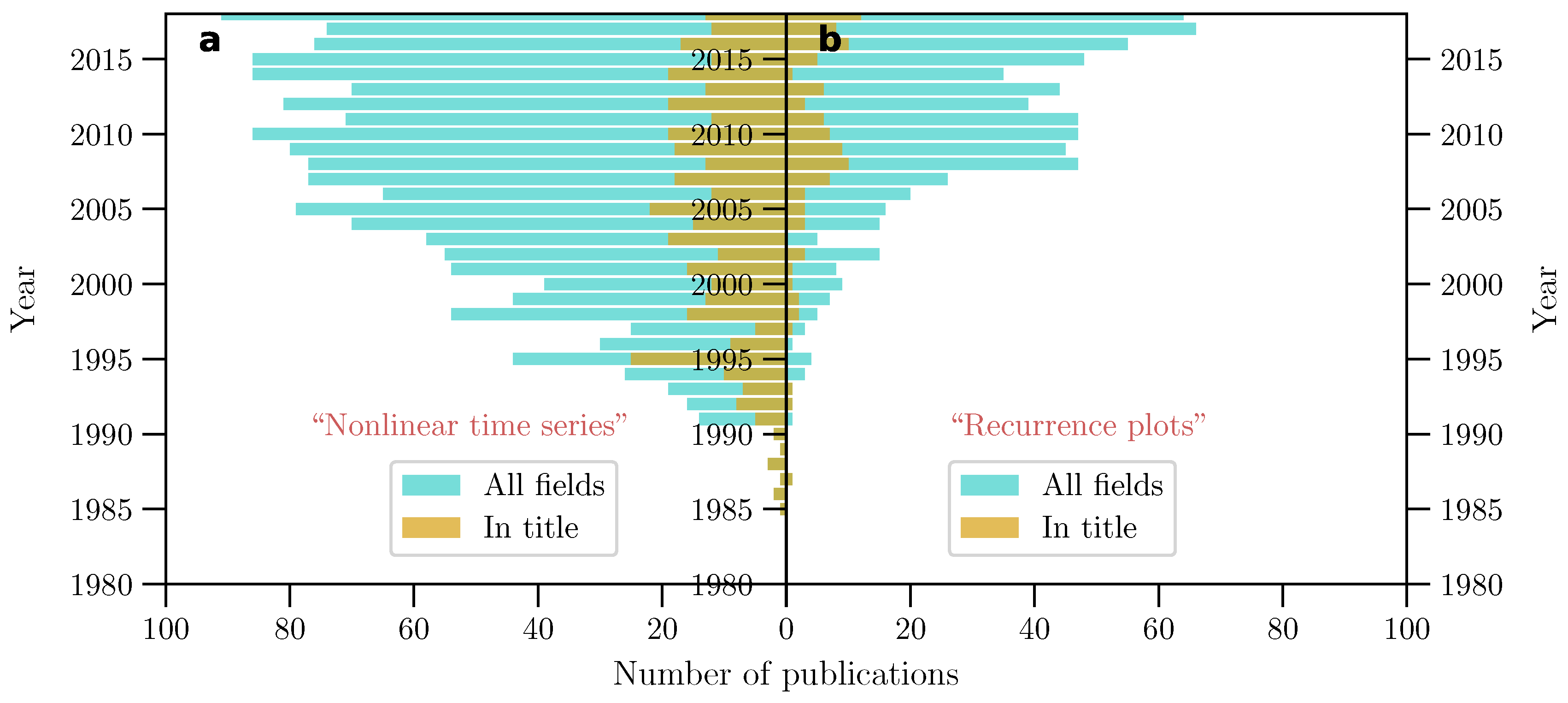
It was not until the early ‘80s, however, that the theoretical developments of nonlinear dynamical systems began to give rise to new time series analysis techniques. This was primarily because most real-world time series were one-dimensional scalar measurements which, in the nonlinear dynamical viewpoint, were the projection of a higher dimensional time evolution on to the set of real numbers by a ‘measurement function’. It was not clear how to infer the details of the high dimensional dynamics in the true ‘state-space’ of the system from scalar-valued time-series measurements. Two papers, one by Packard et al. [2] in 1980, and the other by Takens in 1981 (cf. [3] for a more accessible version of Takens’ original paper [4]), offered possible solutions to this problem and, in essence, gave form to the discipline of nonlinear time series analysis as it is formulated even today. The task of inferring the high dimensional dynamics from a scalar time series, called ‘state-space reconstruction’, became the cornerstone of nonlinear time series analysis. From the 1980s on, along with the further development of theoretical phenomena such as self-similarity and fractal dimensions [5,6,7], strange attractors [8,9,10,11,12], bifurcations [13,14,15], and chaotic synchronization [16,17,18,19], there were an increasing number of studies that applied these concepts to time series obtained from laboratory experiments [20,21,22] and real-world data [23,24,25]. The boom in nonlinear dynamics–related studies is also attributable to the parallel development of increasingly faster, more compact, and more powerful computers (cf. Section 2.9—computers and chaos—of [26]). The 1990s witnessed a drastic increase in the number of studies related to “nonlinear time series analysis” (Figure 1a). Nonlinear concepts began to be increasingly applied to complex systems from different fields such as population ecology [27,28,29], human physiology [30,31,32], and climate [33,34,35].
In 1987, Eckmann, Kamphorst, and Ruelle proposed a new graphical representation, the ‘recurrence plot’, which visualized the ‘recurrences’ of the states of a dynamical system and captured essential features of its dynamics [36]. The recurrence plot was a simple, easily estimable, visual aid to characterize the dynamics of a system. It was based solely on the measured time series and was designed to complement new approaches of the time that estimated various nonlinear dynamical characteristics such as the Lyapunov exponent [37], information dimension [38], and correlation dimension [10]. Over the next decades, however, several methods were put forward to quantify the patterns seen in recurrence plots—e.g., diagonal line structures—to infer probable dynamical features such as a high degree of determinism [39,40,41]. The approaches based on recurrence plots are collectively referred to as ‘recurrence quantification analysis’ (RQA), and they form the core of recurrence plot-based techniques. A crucial advantage of recurrence plot-based approaches over other nonlinear approaches is that they perform reasonably well even when the length of the time series is short (ca. 50–100 data points). Moreover, in cases when the underlying system is not sufficiently deterministic or stationary, recurrence plots have proven useful in characterizing their behaviour.
The intuitive, visual appeal of recurrence plots, and their applicability to time-series from a wide range of systems contributed to a consistent rise in the number of studies involving “recurrence plot” approaches in the last two decades, following the rise in nonlinear time series analysis by roughly a decade (Figure 1b). In addition to studies that extend the theoretical boundaries of recurrence plots themselves, recurrence plot-based approaches have been applied to a wide range of real-world scientific problems from diverse disciplines. For instance, in the field of finance, Strozzi, Zaldívar and Zbilut [42] studied the time evolution of various RQA measures obtained from high-frequency currency exchange data. Bastos and Caiado [43] used RQA to characterize more than twenty stock market indices from around the world and identify changes in the recurrence quantifiers over time, especially during well-known financial crises. In information technological research, Palmieri and Fiore [44] used RQA measures to design a network traffic classification scheme based on the identification of nonlinear transitions in IP traffic flows. Yang, Pan, and Xu [45] used RQA measures to quantify the complexity of the sequences produced by their proposed quantum walk-based pseudorandom number generator for image encryption. Recurrence plots have also been used to study music. Serrà, Serra and Andrzejak [46] used cross-recurrence analysis to design an automated approach that successfully identified cover versions of a given song. Moore, Corrêa and Small [47] use RQA measures to design a surrogate-based hypothesis test which successfully distinguished ten compositions by famous Baroque composer J. S. Bach from a Markov process.
In cognitive science research, Richardson and Dale [48] used cross-recurrence analysis to study the coupling between the eye movements of a speaker, who was told to describe a scene, and that of a listener watching the same scene. Duran et al. [49] used RQA to monitor body movement during acts of deception and found that the upper face, and partly the arms, of a person show less determinism and high complexity while lying. In the field of physiology, Konvalinka et al. [50] analyzed recurrence plots constructed from heart rate data of different subjects present (as active participants and as spectators) during a fire-walking ritual in a tiny rural Spanish village and found that the collective ritual induced synchronized arousal between active participants and bystanders. Acharya et al. [51] used ten RQA measures estimated from electroencephalogram (EEG) data to construct a feature set that was fed into various classifying algorithms to determine the best predictor for epileptic seizures.
Recurrence plots have also been successfully applied to astrophysical and geophysical research. Zolotova and Ponyavin [52] used cross-recurrence plot analysis to investigate phase synchrony between northern and southern sunspot activities. Stangalini et al. [53] applied RQA measures to detect dynamical transitions in solar activity in the last 150 years. Li et al. [54] used joint recurrence plots to investigate the synchronization between a vegetation index and climatic observables and revealed that for most parts of China, vegetation was more synchronized to temperature than precipitation. Zhao et al. [55] conducted a similar study for the Qinghai–Tibetan plateau region using RQA measures and found that vegetation is anti-correlated to the determinism of temperature data and positively correlated to the entropy. A 2003 study by Marwan et al. [56] used cross-recurrence analysis to investigate the influence of the tropical Pacific region on northwestern Argentina using both modern-day and paleoclimatic proxy data sets. More recently, Eroglu et al. [57] applied RQA to speleothem-based paleoclimatic data from two caves in Asian monsoon region and revealed a see-saw relationship in the dynamical regimes between the two data locations. Zaitouny, Walker and Small [58] use recurrence plots in combination with the previously established ‘quadrant scan’ technique [59] to identify tipping points of dynamical systems and demonstrate their approach with real-world examples such as petrophysical data from a geological well in Australia, electrocardiogram (ECG) data recording cardiac arythmia, and EEG data of a person doing a multiplication task.
2. Recurrence Plots in Engineering Research
Recurrence plot-based analyses have also been used in several aspects of engineering research. An early study by Feeny and Liang in 1997 [60] used a recurrence-based generalized autocorrelation function (cf. Zbilut and Marwan [61]) to infer unstable periodic orbits in a stick-slip oscillator model with dry friction. However, the study does not explicitly mention the two-dimensional recurrence matrix that forms the basis of all RQA. In a 2004 study, Wendeker et al. [62] constructed recurrence plots explicitly using pressure time series from a spark ignition engine but they interpreted it only visually to distinguish the observed dynamics from stochasticity. Follow-up studies used RQA measures to show that (i) spark engine dynamics are multidimensional and they change with respect to the spark advance angle [63], and (ii) low (high) frequency crankshaft rotation results in periodic (intermittent) pressure dynamics [64].
Recurrence plot-based approaches have also been used in damage quantification and detection. Nichols. Trickey, and Seaver [65] used multivariate measurements from nine locations on a finite element model of a rectangular steel plate to estimate RQA measures that help to identify dynamical changes induced by a cut (of various lengths) on the plate. Iwaniec et al. [66] used four RQA measures to investigate the changes in dynamics between three different harmonic excitation modes of an aluminum plate and between cracked and uncracked versions of a metal plate. Qian, Yan and Hu [67] estimated a recurrence-based entropy to construct a data-driven model of ball bearing degradation, which they showed could predict failure up to 50 minutes in advance. More recently, Zhou and Zhang [68] constructed a feature vector from four RQA measures and applied it to a control chart [69] which was able to detect faulty ball bearings reliably.
Several studies that investigate the corrosion of metal surfaces with the help of electrochemical noise measurements have applied recurrence plots to distinguish different types of corrosion dynamics. Based on RQA, Garciá-Ochoa et al. [70] showed that an increase in sensitization intensity of S30400 stainless steel led to more deterministic dynamics. Yang et al. [71] showed that higher hydrostatic pressures applied to high strength Ni-Cr-Mo-V steel also induced more deterministic dynamics. Hou et al. [72] used four RQA measures to construct a PCA-based model for detecting corrosion and also as a feature vector for a multilayer perceptron to predict corrosion type. More recently, Barrera, Gómez and Garciá-Ochoa [73] used RQA to assess and compare the performance of protective coatings on cast iron that inhibit corrosion.
Another important application of recurrence-based approaches is in the study of friction-induced vibrations (FIV), in particular with respect to brake squealing and brake noise. Oberst and Lai [74] gave a first quantitative insight into brake squeal noise, using RQA measures to classify and rank noise performance, and showing that (a) linear measures are insufficient to characterize brake squeal dynamics and (b) nonlinear measures reveal that higher nonlinearity leads to a worse squeal. Wernitz and Hoffmann [75] provided a visual interpretation of recurrence plots obtained from friction brake vibration measurements and argued that FIV dynamics are deterministic on short time scales whereas random disruptions were seen on longer time scales. In a recent study, Stender et al. [76] used RQA to demonstrate that FIVs are multiscale in nature, that squealing is consistent with low dimensional attractors, and that the higher vibration levels correspond to higher determinism and periodicity of the dynamics. They also proposed an automated framework based on RQA to detect and monitor brake squealing. In a related study, Stender et al. [77] showed how RQA could help to identify transitions between different types of friction-induced vibration such as chaotic and weakly chaotic epochs, limit cycles and intermittent stick-slip dynamics.
Kabiraj and Sujith [78] used recurrence plots to verify intermittency in their investigation of thermoacoustic instability in combustion systems using a ducted conical premixed flame. Nair and Sujith [79] employed recurrence plots as a visual tool to infer the dynamics of flows in turbulent combustors and infer Type I or Type II intermittency dynamics. Additionally, Nair, Thampi and Sujith [80] showed that RQA measures in swirl-stabilized and buff-body-stabilized combustors could reliably quantify changes in dynamics as a function of Reynolds number and where a potential candidate for early-warning indication of impending combustion. Elias and Namboothiri [81] used cross-recurrence analysis to identify the transition from regular cutting to chatter cutting of metal plates irrespective of the choice of metal. Harris et al. [82] showed that RQA measures were able to characterize the dynamics of bistable cross-shaped laminated plate energy harvesters and proposed recurrence plots as an efficient approach to distinguish different classes of dynamics such as single-well periodic dynamics, chaotic snapthrough, and continuous snap-through. Oberst et al. [83] have recently shown how recurrence-based power spectra could be used to identify stable and unstable periodic orbits in model systems as well as mineralogical deposits in Western Australia. In their study, recurring episodes of low dimensional dynamics and period-doubling route to instability were revealed along the depth axis of the deposits.
3. About This Tutorial Review
The aim of this tutorial review is to provide a brief introduction to the basics of nonlinear time series approaches, with a special focus on recurrence plots. Since the concepts of high dimensional flows, state-space reconstruction, time delay embedding, and dynamical attractors are essential to understand how a recurrence plot is estimated and how its patterns are to be interpreted, this review covers the fundamentals of these topics. An additional crucial concept related to time series analysis is surrogate-based hypothesis testing. The fundamental ideas behind statistical hypothesis testing and the role of surrogate data sets in time series analysis methods are presented and a couple of surrogate methods are discussed. Applications from model systems and real-world systems are used as didactic tools where appropriate.
This review is not the first of its kind, neither in the broader domain of nonlinear time series analysis, nor in the more focussed topic of recurrence plots. I refer the reader to [84,85,86], and more recently [87], for excellent introductions to nonlinear time series analytical thought. For an in-depth overview of recurrence plots as a data analysis tool, the review in [88] is recommended, and for a historic coverage of recurrence plot-based approaches, [89] is helpful. This review is not exhaustive—it is intended to provide only a glimpse into nonlinear thinking. No attempt is made to provide a comprehensive literature survey. Rather, the focus is on illustrating key topics with the idea that the readers are made curious and literate enough to go out and explore on their own. Moreover, the review is biased by my own areas of expertise and relevant pointers to similar approaches developed in other studies are provided when appropriate and necessary.
The remainder of the tutorial review is organized as follows: Section 4 highlights several consequences of moving from a linear to a nonlinear paradigm of looking at the world. Section 5 touches upon the basics of the theory of nonlinear dynamical systems. Section 6 summarises the fundamentals of how nonlinear time series approaches represent the time series data and how we can reconstruct the state-space of the high dimensional dynamics from a scalar time series. Section 7 deals with recurrence-based analysis, outlining the concepts of recurrence plots and recurrence networks and showing how to use them to characterize dynamics, estimate synchronization, and detect transitions. Section 8 illustrates the idea behind surrogate-based hypothesis testing and its necessity in time series analysis of real-world complex systems where we do not have access to multiple realizations of the dynamics. Section 9 demonstrates the discussed approaches with real-world examples from climate, and Section 10 concludes the tutorial review with a brief summary and outlook.
Before we proceed, a brief note on measurement units: Without loss of generality, all measured variables presented in this tutorial review are considered to be scaled such that they are dimensionless. For instance, dividing each value of a signal by the sample standard deviation makes it dimensionless while retaining all dynamical features—the primary focus of the discussion here. In a similar sense, the unit of ‘time’ for all-time series presented here (other than the real-world examples) is arbitrary, i.e., we can choose it to be seconds, minutes, or hours, etc., without impacting the dynamical aspects being explained. Thus, rather than fix a particular unit for time in the model systems and numerical examples, which is a bit contrived in such cases, we drop the unit entirely with the understanding that it bears no direct relevance to the content of the review.
4. Consequences of Nonlinearity
Idiosyncratic nonlinear behavior such as deterministic chaos, bifurcations, phase synchronization, etc. lead to crucial differences in how we approach various aspects of time series analysis. In many cases, nonlinear behavior is not reflected in linear time series measures such as the power spectrum, correlation, mean, and variance (cf. Chapter 1—Introduction: why nonlinear methods?—of [86]). This does not, however, imply that linear measures are redundant. In practice, while working with a time series for which the underlying process is not known, nonlinear approaches are used as complementary tools to linear time series characterization so that we pin down the dynamics as reliably as possible. Four key aspects of time series analysis that are deeply impacted by nonlinearity are discussed below.
4.1. Predictability
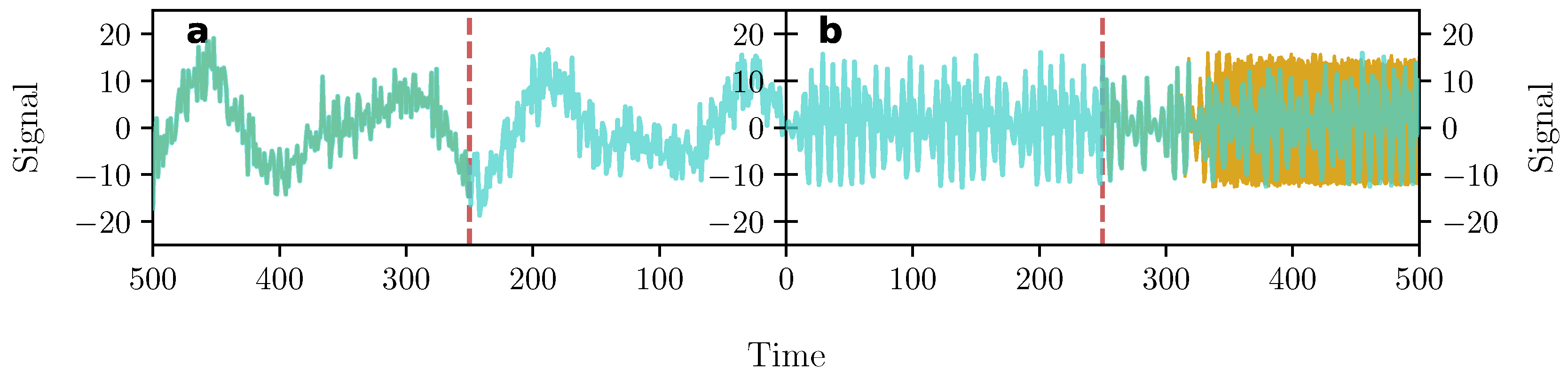
Many nonlinear dynamical systems exhibit ‘exponential divergence’, which means that the distance between trajectories starting from extremely close-by initial conditions increase exponentially as time progresses [90]. This is a necessary (but not sufficient) feature of chaos and has drastic implications for predictability. Imagine we have measured two signals, one that comes from a linear system and is essentially composed of three superimposed sinusoidal frequencies with some additive noise (Figure 2a), while the other comes from a chaotic system (Figure 2b). Now consider the following situation: We measure the time series for both systems up to time and based on this data we determine all three component frequencies of the linear system and we also estimate the exact set of differential equations for the nonlinear chaotic system. We are now in a position to predict the future time evolution of both systems. However, due to the measurement process, our knowledge of the state at time has a miniscule error of the order of times the standard deviation of both signals (which are approximately equal). Due to the exponential divergence of nearby trajectories in the chaotic system, the tiny uncertainty in fixing the initial condition for future predictions at results in a prediction uncertainty equal to the variance of the signal after some time (yellow region in Figure 2b visible from on). In the linear system, the initial uncertainty stays constant throughout the entirety of the future projection. This is one fundamental reason why the weather cannot be predicted more than ten days in advance (on average), even if we were to have immense computational power and high measurement precision.
4.2. Transitions
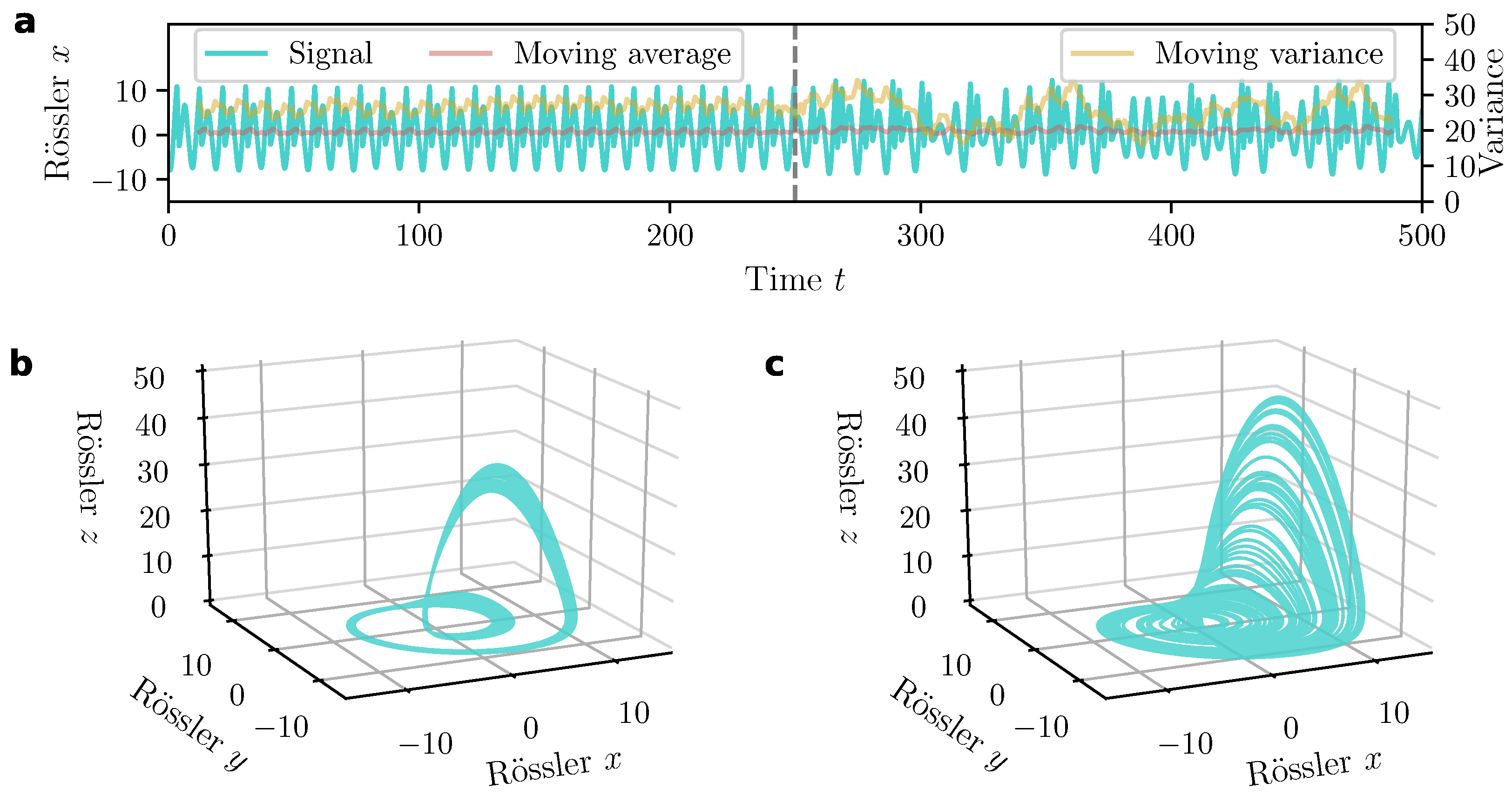
Another important consequence of nonlinearity is that nonlinear processes exhibit non-intuitive transitions between qualitatively different dynamics when system parameters are changed by small amounts. At times, these transitions are not visible in the time series themselves and are also not captured by their statistical moments. To demonstrate this, consider the chaotic Rössler system, a canonical model system that exhibits paradigmatic nonlinear behavior and is often used as a benchmark for testing new techniques of nonlinear time series analysis. We integrate the three-dimensional system of ordinary differential equations for the Rössler system (cf. Equation (1) in Section 5) for two different values of its parameter a, and concatenate their equilibrium values at . Doing this effectively results in a transition at (Figure 3a) from so-called ‘spiral-type chaos’ (Figure 3b) to ‘screw-type chaos’ (Figure 3c). A moving average of 25 time units (yellow line in Figure 3a) fails to capture the transition. The moving variance of 25 time units shows different behavior for the screw-type chaos but it is still not possible to uniquely associate a distribution of variances to each dynamical behavior. To detect transitions in a time series generated from nonlinear processes is not a trivial task, as the dynamical changes can be subtle and non-trivial. Nevertheless, it is important to use as many indicators as feasible to reliably conclude whether or not the system might have gone through a transition.
4.3. Synchronization
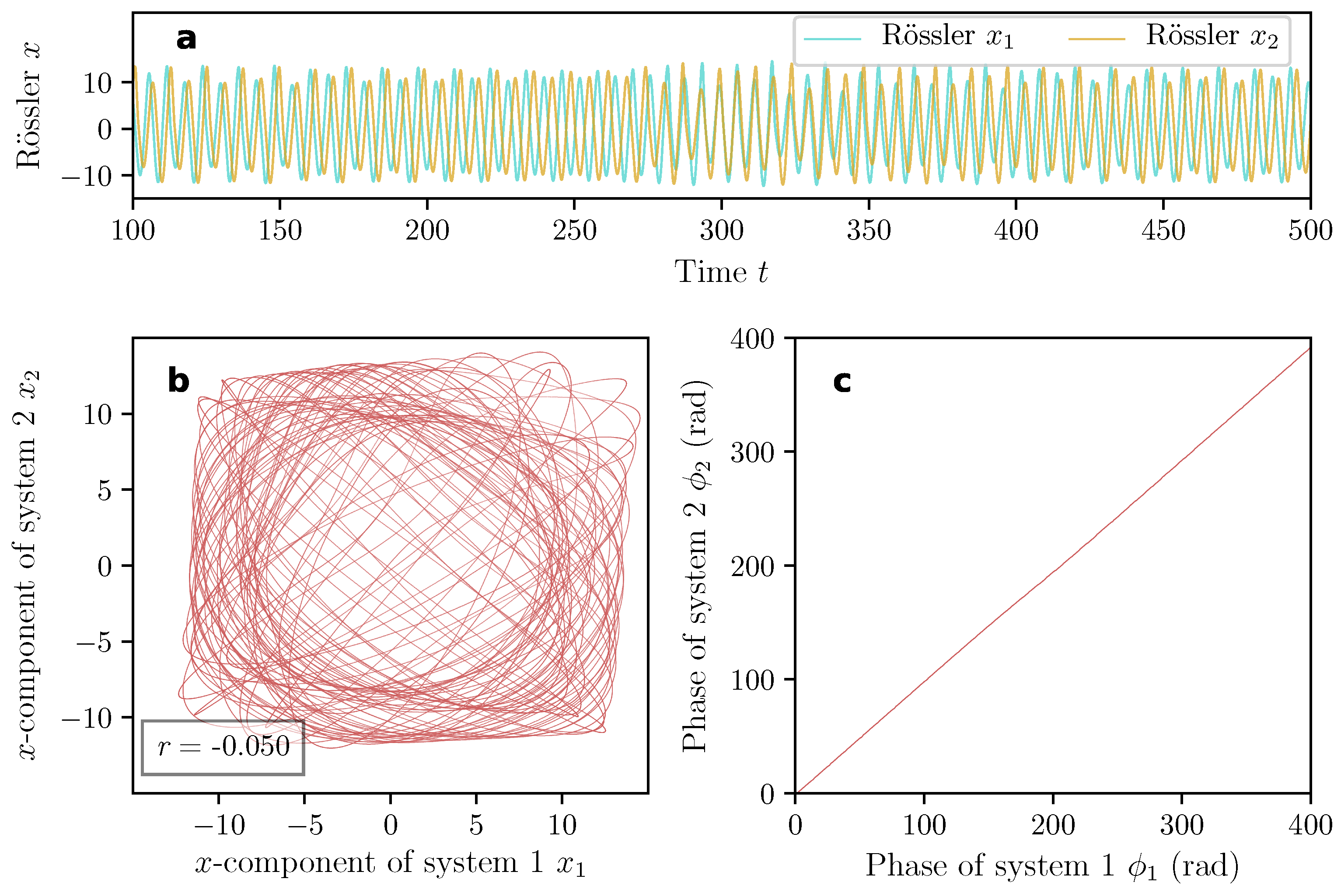
The study of synchronization predates the discovery of chaos and it is a far more general phenomenon found in various systems, both linear and nonlinear. The synchronization of chaotic systems, however, opens newer ways of looking at interdependencies between complex systems. It turns out that there are subtler ways of connecting two systems than by a simple positive or negative correlation. One interesting case is the phenomenon of ‘phase synchronization’, which is a weak form of synchrony between two systems, classically used to study the co-evolution of periodic self-sustained oscillators. That phase synchrony is possible for chaotic systems was first demonstrated in 1996 by Rosenblum, Pikovsky and Kurths [18]. We consider here the same example as used in [18], where two chaotic Rössler systems are coupled in the first variable x and which show phase synchrony for a coupling strength of 0.035 (Figure 4a). Under this condition, the amplitudes of both systems are not correlated (Figure 4b) whereas the phases (as estimated using a Hilbert transform of the x-components) are approximately equal (Figure 4c). In the context of time series analysis, this implies that estimating only the cross-correlation (or even mutual information) of the measured signal (in this case, the x-components of both systems) is not enough to capture all possible forms of interrelations.
4.4. Characterization
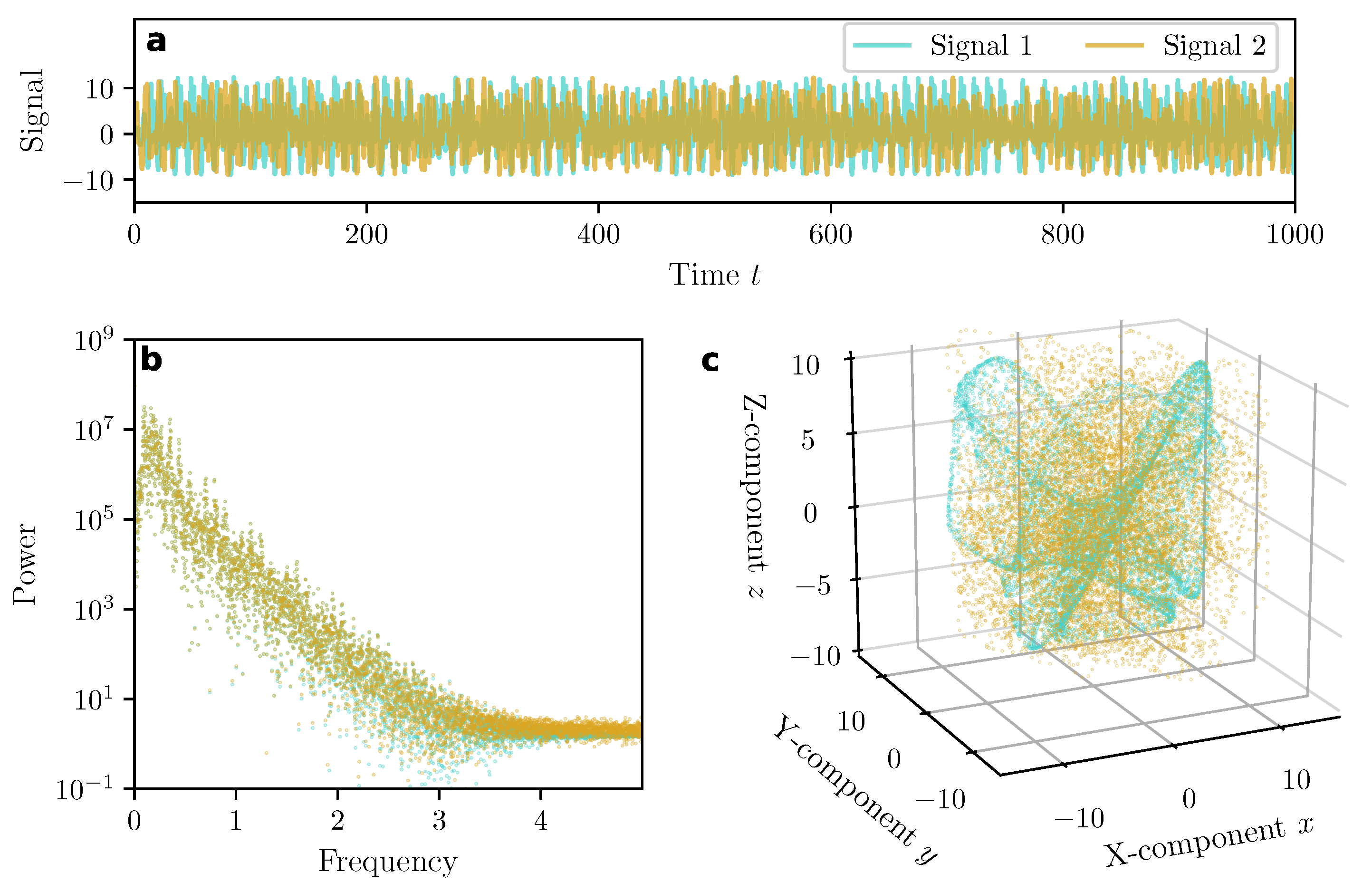
In signal processing, it is common to characterize a time series by its power spectrum, which highlights the dominant harmonic frequencies in the signal by plotting the square of the amplitudes of the Fourier transform of the data against its frequency range. For a linear and time-invariant (i.e., stationary) system, the Fourier transform completely describes the response of the system to perturbations because the complex exponentials of the Fourier transform are also the eigenfunctions of such systems. In certain cases of nonlinearity, this might not be sufficient to describe the entirety of the system’s properties. To illustrate this, we consider two signals (Figure 5a), where one is from the chaotic Rössler system, and the other is a randomized version of the Rössler time series. The randomisation is done using a specific method [91] which ensures that the power spectrum of the randomized signal is the same as the original signal (Figure 5b). The randomized signal, however, possesses none of the complex characteristics in high dimensional time evolution as is seen in the chaotic time series (shown in Figure 5c). Thousands of such randomized versions of the original signal can be generated, each unique in their time evolution, and each with a power spectrum similar to the original chaotic time series. Still, they are, in essence, random processes—sharing none of the determinism of the Rössler system.
5. Dynamical Systems: The Basics
5.1. What Is a Dynamical System?
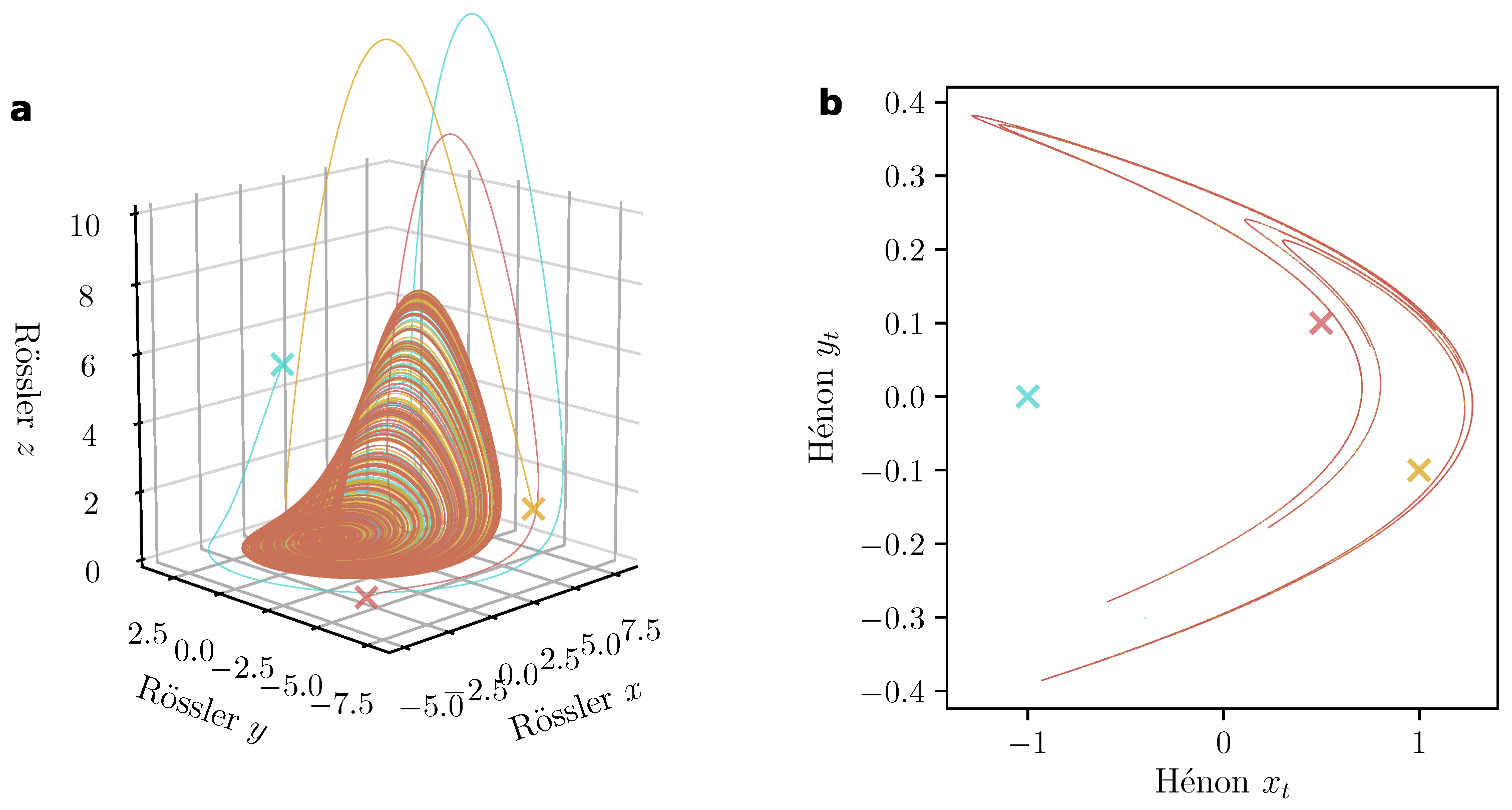
The time evolution of a dynamical system is formulated mathematically in terms of either (i) a system of differential equations that result in ‘flows’, i.e., continuous time-evolving trajectories, or (ii) a system of discrete iterative rules often called ‘maps’. The well known Rössler model already used in Section 4 is an example of a three-dimensional flow and the two-dimensional Hénon map is a well-known example of a discrete map (Figure 6 shows the state space trajectories for the two systems). In both scenarios, the system’s time evolution starts from a prescribed initial condition (crosses in Figure 6a,b) and all subsequent points are obtained according to the integration of the system of differential equations (for the Rösser system) or by using the discrete-time iteration rules (for the Hénon system).
The Rössler model is described by the following equation system:
where denotes the time derivative , and are the parameters of the system (for Figure 6a ). For the Hénon map, the dynamic (i.e., the time evolution) is described by a set of time discrete functions:
where denotes the value of x at time and are the parameters of the system (for the behaviour in Figure 6b, and ). A crucial difference between the two systems is that the system state in the Hénon map ‘jumps’ from one point in the -plane to another at each time step of iteration. However, in the Rössler system, the trajectory ‘flows’, in a continuous sense, from one point in the 3D space to another such that any point in the trajectory is connected to any other point itself by a continuous unbroken path.
The system of equations in Equation (1) can be rewritten more concisely using the following notation. Consider as the vector (in the 3D space ) that describes the state of the system at a given time t. Next, take as the 3D function which maps every point in to another point in itself, and denoting the set of parameters, which in this case is . The three individual functions that compose are the relations given in the right-hand sides of the equations in Equation (1), i.e., . Thus the Rössler model in Equation (1) becomes
which, without loss of generality, can be used to denote the dynamic of any flow. Similarly, we can write down the generic form of the map in Equation (2) as
which again is a generic form used to describe maps. In this particular case, for the Hénon map, , , and . In both cases, given the space , which contains all possible states the system can attain, and the function , which tells us how to move from the state at a time t to a next time (continuous) or (discrete), we have complete knowledge about the time evolution or the dynamics of the system, i.e., the system is fully described. The space is called the ‘state space’ of the system (at times also referred to as the ‘phase space’), and is referred to as the ‘dynamic’ which occurs within the state space. Together, the state space and the dynamic constitute the ‘dynamical system’.
5.2. Attractors
Given a particular configuration of the parameters of a dynamical system, it is found that the equilibrium behavior, i.e., the values of state as time , is either ‘uni-stable’ or ‘multi-stable’. ‘Uni-stability’ implies that, all initial conditions for a given converge to a single type of equilibrium behavior such as fixed point, periodic, chaotic, hyperchaotic, etc. ‘Multi-stability’ would imply that the state-space can be partitioned into mutually exclusive sub-spaces of initial conditions, such that each sub-space converge to a particular equilibrium behavior. In this tutorial review, we consider only the uni-stable case. This is shown in Figure 6, where all three initial conditions chosen for the Rössler system and the Hénon map ultimately ended up in the same region of the state space, and actually even in the same ‘shape’. The set of states in the phase space which determine the equilibrium dynamics irrespective of initial conditions is called the ‘attractor’ of the system for the chosen parameters . An additional condition for the set of states to be an attractor is that once the trajectory of the system reaches this set, it should stay within the set for the rest of the time. There are many different mathematical ways of defining attractors, as also there are different kinds of attractors for different dynamical systems and under different conditions. In general, a few desired properties of attractors are [9,92]:
- Invariance: the attractor should map to itself under .
- Attractivity: any set of initial conditions in the state space should, for large t i.e., , converge to the attractor.
- Irreducibility: the attracting set of states should be connected by one trajectory and it should not be possible to decompose the attractor to subsets of states which have non-overlapping trajectories. In this case, each subset would be an attractor and not their union.
- Persistence: the attractor should be stable under small perturbations, i.e., small deviations from the trajectory on the attractor should return back to the attractor.
- Compactness: the attracting set of states for the dynamic should be compact.
5.3. Bifurcations
Dynamical systems typically exhibit different types of equilibrium behavior when one or more of the system parameters are changed. The equilibrium behavior changes because the change in the parameters destabilizes an existing attractor and new attractors emerge in its place. An added feature of such behavioral changes is that they often happen suddenly, i.e., there typically exists a critical parameter value above and below which the system has two different attractors, or in the case the system is multi-stable, the system might show different configurations of multi-stability before and after the critical parameter value. The parameter value at which the attractors of the system change qualitatively to a different type is called the ‘bifurcating point’ and the phenomenon itself in which the system changes its equilibrium behavior is called a ‘bifurcation’. There are many classes of bifurcations that have been observed in dynamical systems, such as the saddle-node, pitchfork, Hopf, homoclinic, and heteroclinic bifurcations (cf. Chapters 3 and 8 of [90]). Although for algebraically simple dynamical systems, the points of bifurcation can be analytically obtained, in most cases, it is useful to numerically integrate or iterate the system for various values of the bifurcating parameter and plot the ‘bifurcation diagram’. The bifurcation diagram is obtained by visualizing the equilibrium values of one dynamical variable against the parameter value. There are different ways in which a dynamical system approaches a chaotic attractor as the bifurcation parameter is varied. Both the Rössler model and the Hénon map considered here bifurcate when we change their respective parameter a (Figure 7) and approach a chaotic attractor via the ‘period-doubling route’ to chaos [93].
In analyzing time series where the system dynamics are not known, the notion of bifurcations plays an important role as it opens up the possibility of having transitions that do not show up in the statistical moments of the variable but nevertheless involve qualitatively different equilibrium behavior. We have encountered one such scenario in Figure 3 in which the Rössler system undergoes a bifurcation from spiral-type chaos to screw-type chaos. The mean and the variance of the observed time series are similar before and after the transition.
6. State Space Reconstruction
The diverse complex behavior exhibited by nonlinear dynamical systems opened up new perspectives of looking at real-world systems. At the same time, however, it gave rise to a critical problem in the analysis of time series that were obtained from real-world complex systems: how could high dimensional dynamics be analyzed using only scalar time series? One solution to this challenging problem was first proposed in the seminal paper by Packard et al. in 1980 [2], in which the authors proposed to reconstruct the state space from a scalar time series by using the derivatives of the time-series measurements. In the case of noisy measurements, however, derivatives of increasingly higher-order amplify the noise. In this tutorial review, we consider a second approach, first given by Takens in 1981 [4], in which a system of delay coordinates is used to reconstruct the state space dynamics of higher dimensionality. These two papers—by Packard et al. and by Takens—in conjunction with a third crucial addition by Sauer, Yorke, and Casdagli [3] a decade later, laid down the fundamental pillars of nonlinear time series analysis methods. We explain below the time-delay embedding approach to state-space reconstruction, and follow the review in [84] closely, due to its concise, sharp description.
6.1. The Measurement Paradigm and Time Delay Embedding
Consider the dynamical system composed of the d-dimensional state space and the flow which maps a point in the state space at a given time to the next point on the trajectory at the next time instant. We obtain a scalar time series by using a measurement function which maps discrete locations of the d-dimensional flow to discrete, time-ordered scalar values such that , where and is the initial state of the system at time . In this situation, one can define a delay coordinates map [84], , such that , where
Here, maps a point on the flow to a point of the reconstructed state space in with the help of the ‘time delay’ , and the ‘embedding dimension’ m. Takens proved that has the generic property that it is an embedding of in for the condition [4]. That it is an embedding implies that is a diffeomorphism, and that it is ‘generic’ implies that the subset of pairs which result in an embedding is an open and dense subset in the set of all pairs of . Although in principle this was a path-breaking result, for actual high dimensional real-world systems (such as regional weather systems), it meant that the embedding dimension had to be greater than twice the dimension of the state space. This would mean that the scalar time series would have to be extremely long in order to facilitate an embedding in such a high dimension. The next advancement in this regard was made by Sauer, Yorke, and Casdagli [3] where the condition was further constrained so that m needed to be greater only than twice the box-counting dimension of the attractor in order to ensure that it is an embedding of . All such embeddings are “prevalent” rather than “generic” in the sense that ‘almost all’ pairs of will result in an embedding. This result had tremendous practical consequence because a large part of nonlinear dynamical systems were, in fact, dissipative systems in which the volume and dimensionality of the attractor was drastically smaller than the state-space . In other words, since all initial conditions would ultimately settle to the dynamics on , which had a much smaller volume, and consequently much smaller dimension, than , it was possible to study and model the equilibrium dynamics of a high dimensional system using a much smaller dimensional embedding as given in Equation (5).
6.2. Time Delay Embedding in Practice
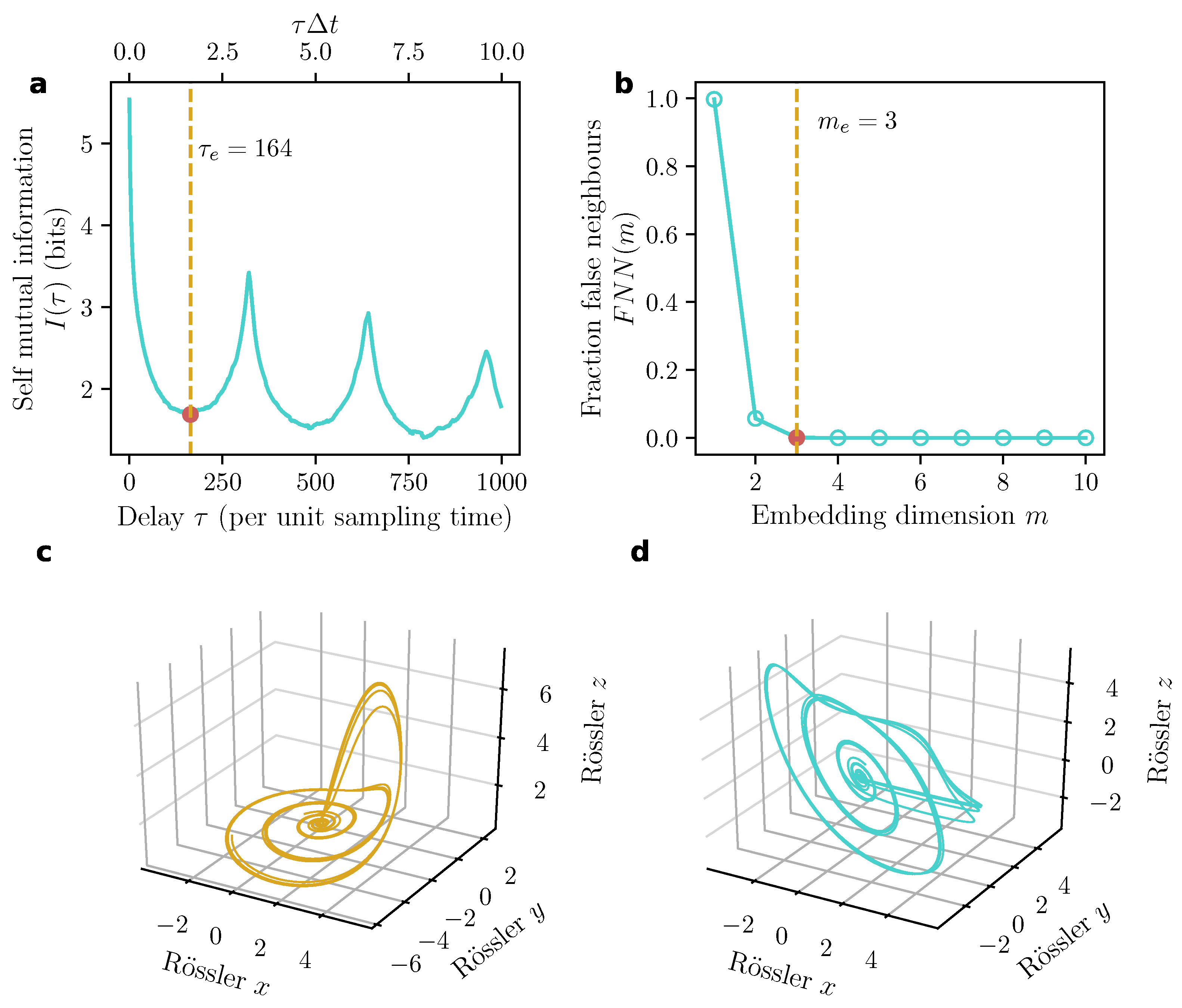
In order to determine the embedding from a given time series, the time delay and the embedding dimension m must be fixed. The results of Takens and Sauer, Yorke, and Casdagli prove the existence of the embedding, but they do not tell us how to determine and m. Till date, there are no rigorous mathematical results that provide a unique route by which to determine these two parameters. In the absence of such proofs, numerous methods have been proposed that use various heuristic considerations to direct the time series analyst on how to optimally choose and m. We focus here on two popular approaches, one each for selecting and m, which allow us to reliably reconstruct the attractor of high dimensional dynamics from scalar time series (Figure 8c,d).
- Determining the time delay. The choice of impacts the resulting embedding critically. When is smaller than the desired value, consecutive coordinates of are correlated and the attractor is not sufficiently unfolded. When is larger than the desired value, successive coordinates are almost independent, resulting largely uncorrelated cloud of points in without much structure. It is important that the fundamental idea in determining the time delay is that each coordinate of the reconstructed m-dimensional vector must be functionally independent. In order to achieve this, it is recommended to set to the first zero-crossing of the autocorrelation function. However, the autocorrelation function captures only linear self-interrelations, and it is more preferable to use the first minimum of the self-mutual information function (Figure 8a), as first shown in [94]. For the scalar time series , the self-mutual information at lag is,where is a random variable underlying the sample and is the random variable underlying the sample . In this notation, the optimal value of is given by,
- Determining the embedding dimension. The method of false nearest neighbours (FNN) put forward by Kennel, Brown and Abarbanel in 1992 [95] is typically used to determine the embedding dimension, once a time delay is chosen. This approach is based on the geometric reasoning that given an embedding in dimension m, it is possible to differentiate between ‘true’ and ‘false’ neighbours of points on the reconstructed trajectory. In this method, we first choose a reasonable definition of ‘neighbourhood’. Based on this definition, we identify the neighbours of all points on the trajectory in . Next, we look for the false neighbours, defined as those neighbours which cease to be neighbours in dimensions, i.e., when we consider the trajectory . The false neighbours were neighbours in the lower dimensional embedding solely because the attractor was not properly unfolded and we were actually looking at a projection of the attractor rather than the attractor itself. As an example, consider the 2D limit cycle trajectory on a circle, where opposite points that are almost on the same vertical line would be seen as neighbours if the same dynamic were projected on to the horizontal axis, i.e., the 1D real line . Once the attractor is properly unfolded, however, the number of false neighbours would go to zero. In practice, this notion is implemented by the following formula (after Equation (3.8) of [86]),where denotes the Heaviside function which is one for all positive arguments and zero otherwise, denotes the maximum norm and is the index of the point closest to in the m-dimensional embedding based on maximum norm. The first term in the numerator counts all those cases when the distance between a point and its closest neighbour increases by more than a factor of r in going from m dimensions to dimensions. However, in order to not count those cases where the points are already far apart in m dimensions, the second term in the numerator is used as a weight and also as a normalisation factor in the denominator. The second term ensures that we count only those cases where the closest neighbour in m dimensions is closer than , where is the standard deviation of the data. The final embedding dimension is the smallest value of m for which the fraction is zero (Figure 8b).
7. Recurrence-Based Analysis
Recurrence-based analysis utilizes a fundamental characteristic of dynamical systems: that a system’s dynamical trajectory eventually returns close to earlier states as time passes. Particularly in the case of time series obtained from real-world systems, we find that systems repeat earlier behavior, even if only in an approximate sense, and even though they might at times be interrupted by regime shifts and dynamical transitions. Poincaré was the first to mathematically describe the recurrence of dynamical systems 130 years ago, known today as the ‘Poincaré Recurrence Theorem’ [96]. As a principle of analyzing time series, however, the first breakthrough for recurrence-based analysis came with the pioneering paper of Eckmann, Kamphorst, and Ruelle [36]. Their work demonstrated, for the first time, how to construct the ‘recurrence plot’, which encoded the pairwise recurrences of time series values, and which created a visual typology of the dynamics, solely from the measured time series. This forms the basis of all of the recurrence-plot-based analysis presented in the sections below. We refer the reader to [88] for a comprehensive review of recurrence plots.
7.1. Recurrence Plots
Consider the dynamical system , as before where is a measured d-dimensional time series of length N. The system is said to recur when a state at time is approximately ‘close’ to a different state at time , i.e., . Here, the notion of being close to depends on (i) the choice of a norm such as the Euclidean norm or the maximum norm, and (ii) the choice of a distance threshold, which helps to unambiguously define all states farther apart than itself as ‘not close’, and vice versa. We can thus encode all possible pairs of recurrences in the recurrence matrix ,
where is an appropriate norm, is the chosen distance threshold and is the Heaviside function. The resulting matrix of size thus a binary-valued matrix comprising solely of 1 s and 0 s, where the 1 s denote pairs of time points where the measured states recur and 0 s denote non-recurring pairs of time points. is symmetric only if the chosen norm is symmetric. In their original paper, Eckmann, Kamphorst and Ruelle [36] used a k-nearest neighbor norm. When we have a single scalar time series , we first embed the time series using time-delay embedding (Section 6) to obtain an embedded state-space trajectory , where . The recurrence matrix is then estimated from the embedded trajectory . A ‘recurrence plot’ is obtained when we visualize the recurrence matrix by placing a black dot for every 1 and an empty dot for every 0. Based on the relatively simple estimation process given by Equation (9), we arrive at a powerful visual representation that captures the difference in dynamical behaviour (Figure 9). The recurrence matrix contains all relevant dynamical information. Robinson and Thiel [97] proved that, given a recurrence matrix , it is possible to reconstruct the time evolution of the dynamical system up to a homeomorphism, i.e., up to a change in the coordinate system. This result is practically observable in the successful reconstruction of time series and attractors from recurrence plots [98,99].
To construct a recurrence plot (RP), however, one has to carefully choose the various parameters related to the estimation of in Equation (9). The embedding parameters and have been extensively studied for their influence on recurrence plot-based estimates. Iwanski and Bradley [100] demonstrated that that for particular low dimensional systems, RQA measures remained unchanged on change of embedding parameters, and Thiel et al. [98] showed that the estimation of second-order Rényi entropy and the correlation dimension from recurrence plots was independent of the choice of embedding. However, this is not the case for all RP-based estimates. March, Chapman and Dendy [101] derive analytical formulae that explicitly express two recurrence-based measures (indicative of deterministic behavior) as a function of the embedding dimension. Thiel, Romano, and Kurths [102] also report how over-embedding—the choice of embedding dimension much larger than the minimum required to unfold the attractor—can introduce spurious correlations between the embedded vectors.
The choice of the parameter impacts further analyses based on , and there is no mathematical result which prescribes how to choose uniquely. There are several studies that have proposed approaches to decide on an optimal [103,104,105,106,107]. As a general rule of thumb, it is best to choose such that the recurrence matrix does not have too few 1 s (empty recurrence plot) or too many (almost completely filled recurrence plot). The ratio of the number of 1 s to the size of , known as the recurrence rate, is typically kept in the range of 5–10% for most analyses. The choice of is innately linked to the timescales that we wish to investigate. On increasing , we increase the tolerance of what constitutes a recurrence, and end up with more 1 s in , which fills in finer, and shorter timescale, structures from the recurrence plot. If the focus of the study is to study longer timescale behavior, increasing the recurrence rate beyond 30% might be appropriate.
Irrespective of the final chosen value of the parameters , , and used to construct a recurrence plot, sensitivity tests have to be carried out. A sensitivity test (with respect to one parameter) is typically done by changing the parameter value up to a few percent of the value chosen for the main analysis. The results would indicate whether or not the final conclusions are robust to small changes in parameter values.
Beside univariate time series, recurrence plot analyses can also be extended to bivariate data using cross-recurrence plots [108] and multivariate data using joint-recurrence plots [109]. Other than cross- and joint-recurrence plots, additional extensions of recurrence plots include windowed- and meta-recurrence plots [110] weighted recurrences plots [111], fuzzy recurrences plots [112], order pattern recurrence plots [113], and recurrence plots of recurrence plots [114]. Each of these extensions provide useful insights into the recurrence features of idiosyncratic dynamical systems.
7.2. Recurrence Networks
In 2009, Marwan et al. [115] proposed an extension to recurrence plot-based analysis. Their approach was to exploit the inherent analogy between the adjacency matrix of a network and a recurrence matrix to define a new object, the ‘recurrence network’, which is the network represented by the adjacency matrix obtained by removing the main diagonal of the recurrence matrix , i.e.,
where is the Kronecker delta, which is 1 when and 0 otherwise. Removing the main diagonal from is equivalent to removing self-loops in the recurrence network—a necessary condition to analyze several ‘path’-based measures in order to avoid getting stuck in an infinite loop. The recurrence network is thus the network obtained when we consider the states as the nodes of the network and place a link between and all other states which are closer to it than the chosen threshold . The network itself is embedded in the state space of the dynamics (or in the embedding space for reconstructed attractors), and is similar to the phase space networks described by Xu, Zhang, and Small in their 2008 article [116]. In the last decade, recurrence networks have been applied successfully to reveal nontrivial dynamical features in various complex systems [117,118,119].
In general, considering the recurrence patterns of a nonlinear dynamical trajectory as a complex network results in a paradigmatic shift in how we phrase the dynamical questions (synchronization, transitions, and so on), and enables us to apply the entire toolbox of complex network-based measures to the time series under investigation. For instance, consider the 2014 study by Eroglu et al. [111], in which the authors propose an intuitive criterion for choosing : that the recurrence network should remain connected. In this way, there exists a critical value of below which the network ceases to be connected, and a value just above this critical value is recommended for . We refer the reader to [120] for an overview of complex network techniques used in time series analysis.
7.3. Quantification Based on Recurrence Patterns
Different structures in recurrence plots are interpreted as characteristics of different kinds of dynamics. Bradley and Mantilla [121] show how unstable periodic orbits can be used as a basis set for the geometry seen in a recurrence plot and how a comparison of the block structure between two RPs can indicate the (dis)similarity between the underlying dynamics. Zou et al. [122] use RPs to distinguish quasi-periodic, fully chaotic, and sticky chaotic orbits in nonintegrable Hamiltonian systems using far less data than other methods. Facchini, Kantz, and Tiezzi [123] show that characteristic curved patterns in an RP can be caused by nonstationarities in the signal, in particular by a linearly increasing or a periodically modulated carrier frequency, and that such nonstationarities are not captured in a traditional spectrogram. More recently, Hutt, and beim Graben [124] propose a new RP-based approach that can identify metastable attractors and heteroclinic orbits, a task that is typically challenging using standard methods.
In general, there are various measures that attempt to quantify different aspects of the recurrence plot into a single number, and they are collectively referred to as recurrence quantification measures. The measures based on recurrence plots typically require the time-ordering information of the recurring points and can thus be considered to capture dynamical features. Measures derived from recurrence networks, however, do not require the time-ordering information, and capture various aspects of the geometry, i.e., the topology, of the attractor. In this section we consider two measures, viz. ‘determinism’ and ‘average shortest path length’, one each from the recurrence plot and recurrence network frameworks.
- Determinism. A prevalent feature found in most recurrence plots are diagonal lines, which show up when there are periods in which trajectories evolve in parallel to each other. A diagonal line of length l occurs when the following condition is satisfied: , , , …, . This condition can hold only when the two sections of the trajectory—one between and and the other between and are parallel to each other in the reconstructed state space, which occurs for periodically repeating portions of the trajectory. A higher number of such periodically repeating sections of the trajectory would imply that the state of the system can be predicted on timescales equal to the period of oscillation which, in this example, would be the time difference . Diagonal lines are thus typically used as an indicator of deterministic behavior, as is also seen in the recurrence plots given in Figure 9. To quantify the extent of determinism contained in the recurrence plot, the recurrence plot-based measure is defined as,where the denominator is the total number of recurring points, is the number of lines of length l, and is the minimum number of points required to form a line. Although technically should be 2, higher values can be chosen in certain cases. For instance, in noisy systems, one can expect very short diagonal lines to occur purely by chance. Such lines do not encode determinism of the system and are better avoided in the estimation of . In such situations, we an set to a larger value so as to count only longer lines as they are less likely to occur due to randomness and more likely to indicate (any) deterministic component of the underlying process. gives a number between 0 and 1 such that a periodic signal (e.g., a sinusoid) will have a value of 1 and a purely stochastic signal will result in a value extremely close to 0.
- Average shortest path length. A ‘path’ between two nodes i and j in a network is defined as a sequence of nodes that needs to be traversed in order to go to node j from node i. In general, there exist many possible paths between any pair of nodes in a network, and there can be even several possible shortest paths between a pair of nodes. However, it is possible to uniquely define a shortest path length between two nodes i and j which is the smallest number of nodes that need to be traversed in order to reach j from i. Often the average shortest path length is a characteristic feature of networks that can help distinguish the topology of one network from another. In recurrence networks, shortest path length helps to characterize the topology of nearest-neighbor relationships. Each shortest path is the distance between two states i and j of the system measured by laying out straight line segments between them such that: (i) each line segment cannot be more than units long, and (ii) the ends of each line segment must lie on a measured state, the first and last of which are i and j respectively. Thus, is bounded from below by the straight line between the states i and j, i.e., is the upper bound for the Euclidean distance between two states on the attractor [115,117], and its average value is an upper bound for the mean separation of states of the attractor [117]. The average shortest path length, , is estimated as—where N is the size of the recurrence network and the normalization factor is the possible number of unique paths between N nodes. In order for Equation (12) to be estimable, we should not have self-loops in the network, which is ensured by Equation (10), and the network also has to be connected, in the sense that must exist at least one path between any pair of nodes in the network. Note that quantifies the topology on the recurrence networks embedded in the state space and in several situations, such as multiple attractors existing for the same parameter set, can help quantify differences between the different attractors based on their geometric layout. This might not be reflected in estimations of mean separation of states for the same attractors.
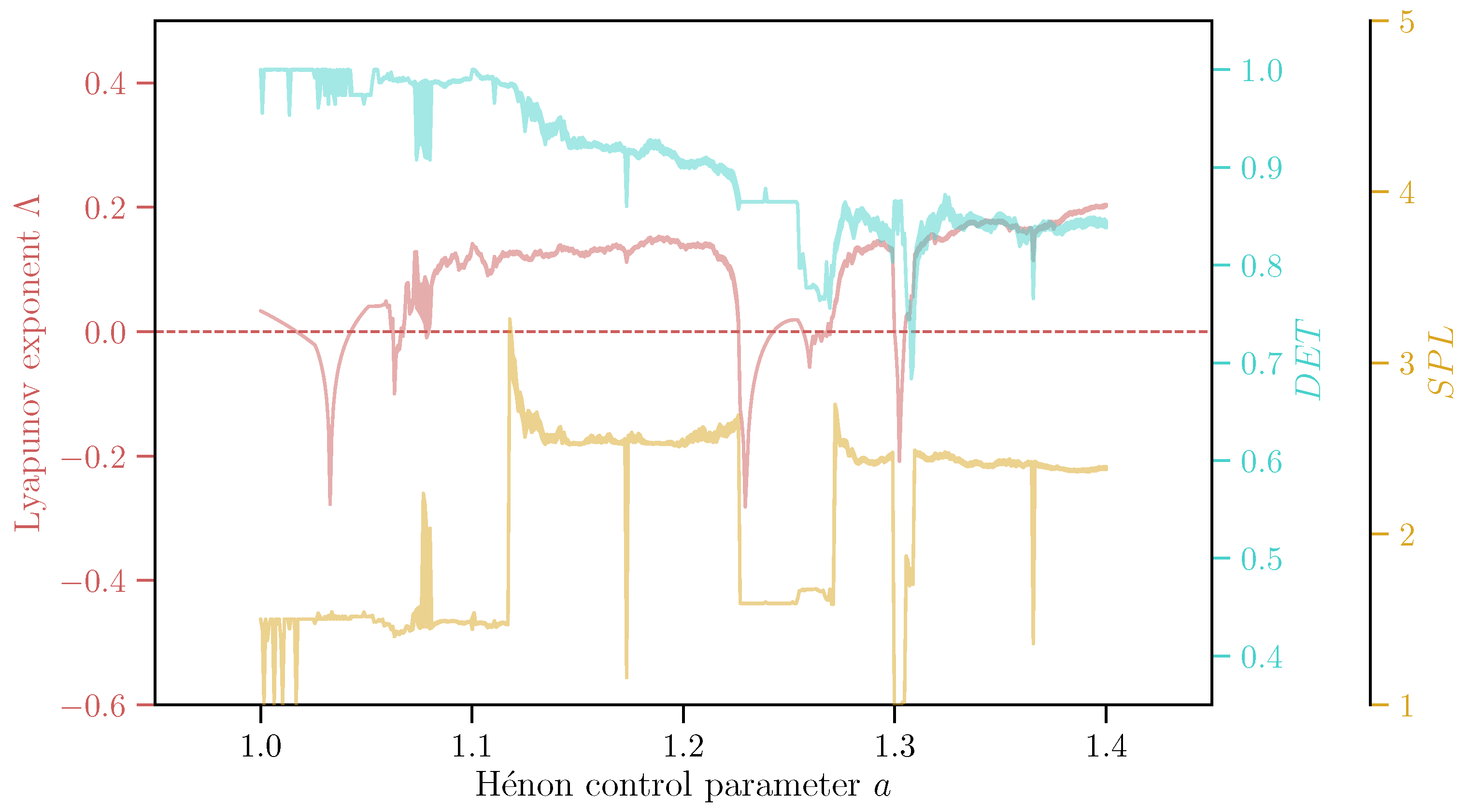
To illustrate the two recurrence-based quantifiers introduced above, we estimate and for the Hénon map for different values of the parameter a between and , and compare the results with the ‘maximal Lyapunov exponent’ (MLE) in each case (Figure 10). The MLE is typically used to quantify the exponential divergence of trajectories:
which for the x-component of the Hénon map translates to,
Values of indicate chaotic attractors where nearby trajectories diverge exponentially as time progresses. Negative values denote periodic attractors where all trajectories eventually converge to a fixed number of states.
We find that tends to decrease from as the map bifurcates towards the chaotic attractor at (green shaded area in Figure 10), and it typically shows a trend opposite to that of the MLE (red shaded area in Figure 10), which increases with a. has low values till around , at which point it jumps to a higher value and then gradually decreases as a is increased. In the periodic windows (ca. for instance), increases sharply and there is a corresponding drop in . Together, the two measures help to infer the underlying dynamics meaningfully: While the decrease in from on tells us that the equilibrium dynamics turn more and more irregular, the decrease in informs us that the attractor shrinks in volume in the same interval.
7.4. Inferring Dependencies Using Recurrences
Recurrence plots also provide powerful ways to determine interdependencies between two systems based solely on the measured time series. Particularly for chaotic oscillators, it can detect subtle and nontrivial modes of connectedness between two systems, such as phase synchronization (cf. Section 4.3) and generalized synchronisation [125]. To detect such forms of synchronization without knowledge of the system equations or system parameters is a difficult inverse problem that becomes potentially tractable with recurrence plots. Romano et al. [126] showed how conditional recurrences obtained from recurrence plots can be used to detect coupling directions whereas Feldhoff et al. [127] estimated coupling directions by a comparison of geometric motifs in the recurrence networks of coupled dynamical systems. Groth [128] showed that a combination of cross-recurrence plots and order recurrence plots can lead to a robust estimator of coupling between two systems. Tanio, Hirata and Suzuki [129] used recurrence plots and combinatorial optimization to reconstruct a slowly varying driving force by observing only the driven system. Hirata and Aihara [130] presented an approach to detect common driving forces from bivariate time series measurements by using counts of joint recurrence of the two systems that were in excess of what was expected from their individual recurrence rates. More recently, statistically motivated measures of interdependencies were proposed which attempt to formulate a mutual information–like quantity based on recurrences [131,132]. Here, we briefly present the measure to detect phase synchronization proposed by Romano et al. [125] and the statistical measure for interdependence proposed by Goswami et al. [131].
- Correlation of probabilities of recurrence. The determination of the phase from the measured time series of a chaotic oscillation is a challenging task. Especially in the case when the attractor is in a non-phase-coherent dynamical regime, it is nontrivial to determine which particular combination of the state space variables would result in a reliable definition of the ‘phase’ of the motion, in the sense that with every time period, the phase should increase by . In their study, Romano et al. [125] exploit this idea to note that for complex systems, we need to relax the condition (which is true for a purely periodic system with a single well defined period ) to rather have , i.e., , which allows us to define the function,where the normalisation ensures that the average number of recurring points for every possible period is considered. The function , also referred to as the -recurrence rate, can be considered as a kind of generalized autocorrelation function of the system which peaks at multiples of the dominant periods of the dynamics (cf. [61]). An important point here is that should be typically greater than the correlation timescales of the system. To estimate the extent of phase synchronisation, Romano et al. suggest to use the Pearson’s cross-correlation coefficient of the and curves from two dynamical systems and in combination with an appropriately selected so-called Theiler window [133] to take into account the autocorrelations of the dynamics. This was updated in a later study [134] to consider only those values , where is the maximum of the two decorrelation times for the two systems, where the decorrelation time was considered as the smallest value of for which the autocorrelation function is less than . Here, we suggest to consider the decorrelation time with respect to instead of the autocorrelation function, i.e., . Thus, the phase synchronisation between and can be obtained by,where and denote the sample mean and standard deviations, and the tilde symbol is used to denote estimates based on the condition. Equation (16) is thus nothing but the sample cross-correlation coefficient of the values obtained for and .
- Recurrence-based measure of dependence. Goswami et al. [131] recently proposed a statistically motivated measure of dependence based on recurrence plots. This idea was further developed by Ramos et al. [132] to include conditional dependences as well which helped to identify and remove ‘common driver’ effects in multivariate analyses. The so-called recurrence-based measure of dependence ( in Equation (20) below) is the mutual information of the probabilities of recurrence of two dynamical systems and . Consider the recurrence plot constructed from the measured/embedded series : we can estimate the probability that the system recurs to the state at time as,and similarly, we get for system . Now, consider the joint recurrence plot [88],which encodes the joint recurrence patterns of systems and by looking at those pairs of time points where a recurrence in coincides with a recurrence and vice versa. The joint recurrence plot allows us to define the joint probabilitywhich encodes the joint probability that recurrences of the system to its state at time coincide with recurrences of system to its state at the same time . The three quantities , , and allow us to define the mutual information of these probabilities of recurrence, i.e.,which encodes the extent to which and are non-independent. For the case where the two systems are completely synchronized, , which means, according to Equation (20), , i.e., the Shannon entropy of the recurrences of states of the system. If the systems are independent, is zero as the joint probability is simply the product of the two individual probabilities of recurrences. We can understand this by observing that the product in Equation (18) involves the element-wise product of two corresponding columns of the individual recurrence plots. For independent systems and , this amounts to estimating the probability of getting overlapping 1 s from multiplying two binary series where the 1 s in each series have been distributed independently according to probabilities and respectively, which is simply .
To illustrate how and work, we consider two mutually coupled Rössler oscillators (after [88], cf. Figure 43C and Equations (A7) and (A8) of that paper) connected bidirectionally in the first component by a coupling strength —
where the parameters and . For the phase synchronous state shown in Figure 4, the coupling strength , but in the current example, we vary the coupling strength in the interval . For each value considered, we integrate the coupled system until it reaches equilibrium behaviour, and consider the last part of the time series for the recurrence plot-based interdependence analysis, i.e., the estimation of and (Figure 11). We take the first components, and , as the observed time series and embed them according to the steps in Section 6. We find that begins to rise as the system approaches phase synchronisation and at , it hits 1 and remains at that value for all higher values of . records a jump at the onset of phase synchrony, which is followed by a noisy plateau till . further shows the onset of lag synchronisation at after which its fluctuations plateau off again. In the interval , the values of show large fluctuations primarily due to intermittent lag synchronisation. In general, behaves similar to the measure put forth in [125] but is easier to implement and faster to compute. For comparison to and , we also estimate the Pearson’s cross-correlation coefficient ,
where and denote the sample mean and standard deviations of and as before and N is the length of the time series. dips sharply to moderate negative values before the onset of phase synchronisation but fails to detect the onset of phase and lag synchronisation (red area in Figure 11).
7.5. Detecting Dynamical Regimes Using Recurrences
Recurrence-based approaches can also be used to distinguish between various dynamical regimes. Casdagli [110] proposed a change point detection measure based on a conditional probability that estimates the likelihood of observing recurrences in two block diagonal squares whose upper-right and lower-left corners touch at the time point being tested for being a potential change point. Beim Graben and Hutt [135] propose to identify change points using a phase space partition constructed as a union of intersecting balls along the trajectory of the dynamics. Rapp, Darmon and Cellucci [59] use a similar notion and propose the ‘quadrant scan’ method to detect transitions, which has been recently also applied by Zaitouny et al. [58] to detect transitions in various kinds of real-world data. Iwayama et al. [136] proposed a change point detection approach based on the detection of ‘communities’ in recurrence networks using spectral clustering. More recently, Goswami et al. [137] use a similar notion and propose that communities can be used as an indicator of abrupt transitions in time series.
All of the above approaches have one thing in common: the idea that block structures in the recurrence matrix correspond to epochs where the trajectory is ‘trapped’ in a particular part of the state space. Identification of block structures, and in particular, the bottleneck time points between two consecutive blocks indicate the change point. Formally, the identification of block structures in a recurrence matrix is equivalent to identifying ‘communities’ in the corresponding recurrence network. ‘Community’ is used here in the sense of Newman’s definition [138], which corresponds to groups of nodes in a network that are more densely linked to each other than the rest of the network. Below, we use the simplest form of identifying a network community, ‘modularity’, to identify abrupt transitions and dynamical regimes in a given time series.
Newman and Girvan [139] put forth the notion of modularity to provide a quality criterion that allowed the inter-comparison of a set of given network partitions (i.e., a community structure) to determine the partition with the strongest community structure, i.e., the highest modularity. Given a network and a partition of the network, modularity estimates the deviation of average within-community link density of the given partition from that of a random network with the same degree sequence. For the adjacency network , let M denote the total number of links in the network, then the modularity is
where is the ‘degree’ of node i defined as the total number of links attached to node i, and is is an indicator function that gives the community index of node i such that equals 1 when and belong to the same community and zero otherwise. In order to evaluate the modularity , we need to thus specify a partition of the network such that different nodes are grouped into different communities. This idea is used to construct an optimisation algorithm which, given all possible communities for a given network, returns the partition that maximizes which serves as a utility function for the maximisation algorithm. There are several algorithms which carry out this optimisation in reasonable computation time. Besides modularity, which is known to have several drawbacks in detecting block structure in networks, many other methods have been proposed to identify communities in complex networks, and we refer the reader to [140] for a comprehensive overview of this topic.
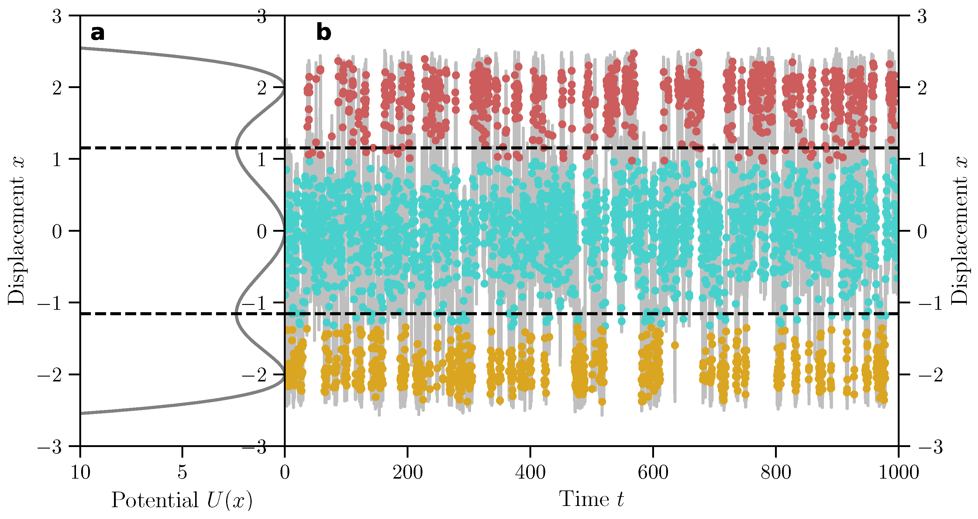
We demonstrate the approach with the example of a particle moving under a symmetric triple-well potential—
with , and (Figure 12a). Based on the Langevin equation for a particle moving under the potential U,
where denotes the magnitude of the stochastic Wiener process , we esimate the time series for the particle’s location by integrating Equation (26) with the Euler-Marayama method:
where , and is a standard normal random variate. Using the fast greedy implementation in Python package for igraph [141] for detecting the communities in a given network while optimizing Newman’s modularity, we obtain three distinct communities (Figure 12b) which almost always correspond to the three stable states around the three minima of the potential U.
8. Surrogate-Based Hypothesis Testing
All-time series analysis essentially involves the estimation of quantifiers from data and subsequent inference of dynamical characteristics. In practice, however, time series quantifiers often yield values that are intermediate and which make it infeasible to formulate an unambiguous inference from the value alone. For instance, if we obtain a value of we are unable to clearly conclude whether the underlying dynamics are deterministic () or random () (cf. [104]). The ambiguity of such time series quantifiers can be tackled in two different ways, which correspond to two different situations of obtaining time series.
First, consider the situation that we obtain our time series from an ‘active experiment’, where we can change the parameters and initial conditions of the system and obtain further time series if necessary. In this case, we can try to identify a bifurcating parameter of the system, and change its value incrementally. We can estimate corresponding to each value of the bifurcating parameter, and compare them with each other (this is the situation in Figure 10). This way, we gain an understanding of which configurations of the system are more deterministic and which are less so. Active experiments allow us to explore time series characteristics on a relative scale simply by enabling us to investigate the system dynamics under different parameter configurations. The second situation is that of a ‘passive experiment’, where we have only one realization of the system, and where we cannot generate a new time series for different system configurations. This is the case for most real-world time series. In the case of such passive experiments, we have to rely on the framework of statistical hypothesis testing, and we have to use ‘surrogate time series’ to help us carry out the tests.
Surrogate time series are randomized versions of the original time series that retain a few desired characteristics of the original dynamics. The characteristics which they retain encode a ‘null hypothesis’ against which we test the ‘significance’ of the time series characteristic. The simplest surrogate generation method is to shuffle the values of the original time series, which destroys all time-ordered dynamical information but retains the value distribution. We can use this method, for instance, to test whether the estimated from a time series is statistically significant under the null hypothesis: the observed determinism is explainable by a random process with a similar value distribution. A second surrogate generation technique was used in Section 4.4 (Figure 5), where we used the Iterated Amplitude Adjusted Fourier Transformed (iAAFT) method [91] to create stochastic time series such that all dynamical structure of the input Rössler data was removed but nevertheless the power spectrum remained unchanged. In this case, the null hypothesis is: the observed dynamical characteristics (, , and so on) are explainable by a random process with a similar power spectrum. To test the significance of measures of interdependence, such as , , or , we typically use twin surrogates [142], which mimic trajectories from the same dynamical system albeit with random initial conditions. Twin surrogates retain both linear and nonlinear characteristics as the original time series, but by virtue of being a trajectory from a randomly chosen initial condition, the coupling is broken. The null hypothesis for twin surrogates is: the observed coupling is explainable by a randomly chosen trajectory, i.e., an independent realization, of the same dynamical system. If the observed value of or is not likely from a randomly chosen pair of twin surrogates, then we fail to accept the null hypothesis, indicating that the observed value of or are ‘statistically significant’, i.e., extremely less likely to have occurred simply by chance from systems that are dynamically similar. We refer the reader to [143] for a comprehensive overview of the multitude of surrogate time series generation methods that have been proposed till date.
In practice, in order to use surrogates for statistical hypothesis testing, we do the following:
- Estimate the time series analysis quantifier Q from the original time-series, denote it as .
- Generate K surrogate time series using an appropriate surrogate generation method.
- Estimate the same quantifier Q from each of the surrogate time series in the exact same manner as was done for the original time series. This results in a sample of K values of Q, which we denote as .
- Estimate the probability distribution from the sample using a histogram function or a kernel density estimate. This distribution is known as the ‘null distribution’ as it is the distribution of values Q for the situation the null hypothesis is true, i.e., for whatever characteristic the surrogates preserve.
- Using , estimate the so-called ‘p-value’, defined as the total probability of obtaining a value at least as extreme as the observed value , i.e.,The p-value encodes how less likely is the observed value to be obtained from the null distribution .
- Based on a chosen confidence level of the test , determine whether is statistically significant at level by checking whether or not. When , the observed value is statistically significant with respect to the chosen null hypothesis, and we fail to accept the null hypothesis, indicating that the observed is caused by characteristics other than what is retained in the surrogates. By convention, is typically chosen at 5%, i.e., or in some cases at 1%, i.e., . Values of higher than 5%, such as 10%, is not recommended as the statistical evidence in such cases is rather weak.
- In cases when there is more than one statistical test, we have to take into account the problem of multiple comparisons. This situation commonly arises in a sliding window analysis, where we divide a time series into smaller (often overlapping) sections and estimate the quantifier Q for each section. If , then 5% of the windows are possibly false positives. To reduce the effect of false positives, ‘correction factors’ such as the Bonferroni correction or the Dunn-Šidák correction are used [144]. In particular, Holm’s method [145] is preferable as it does not require that the different tests be independent. The fundamental idea behind correction factors is to use a corrected value of which is far lower than the actual reported , thereby reducing the effective number of false positives at the reported level of confidence.
It is important to keep in mind that the final inferences are only as strong as the chosen surrogate method and the corresponding null hypothesis. If we estimate from a time series and test its significance against a generated from a simple random shuffle of the time series, then a statistically significant result can only let us conclude that the observed levels of determinism are not likely caused by an uncorrelated stochastic process with the same value distribution. However, if we observe a statistically significant value of against a generated from iAAFT surrogates, then we can make a stronger inference, viz., that the observed levels of determinism are not likely caused by a stochastic processes that possess not only the same value distribution but also the same autocorrelation structure. This would indicate that the determinism is likely due to factors other than the autocorrelation of the dynamics. To test whether an observed value of is significant or not, twin surrogates would not make sense because they give us dynamically similar trajectories which presumably, also have similar values of . To test the significance of against a null hypothesis which gives surrogates with similar values is a contradiction in itself. That said, we can, however, keep increasing the characteristics retained by the surrogates—value distribution, power spectrum/autocorrelation, mutual information, neighborhood structure, and so on—and make the inferences accordingly stronger, as long as the increase in the strength of inference is relevant to what we want to learn from the time series.
9. Application: Climatic Variability in the Equatorial and Northern Pacific
We apply the concepts discussed in the previous sections to the climatic variability of the Pacific Ocean, particular of the equatorial Pacific and the North Pacific basin. The sea surface temperatures (SSTs) in these two regions reportedly impact climatic conditions and weather patterns globally [146,147,148]. SSTs in the equatorial Pacific exhibit the well known El Niño southern oscillation (ENSO), which is an oscillatory behavior between anomalously warm and anomalously cold SSTs on typically quasi-biennial timescales. Anomalous warm (cold) periods in this region, are known as El Niño (La Niña) years. Here, we use the Niño 3.4 climatic index [149], constructed by averaging the monthly SST values in a pre-defined spatial box along the equatorial central Pacific roughly north of Tahiti, between 120W–170W and 5S–5N. The North Pacific basin, roughly the region north of Hawaii and contained between the Asian shoreline to the west and the northwest American shoreline to the east, exhibits a slower timescale oscillation known as the Pacific Decadal oscillation (PDO) [150]. An index for the PDO is estimated from the leading empirical orthogonal function (EOF) pattern of SST anomalies in the North Pacific basin. The positive (negative) phase of the PDO typically has a cold (warm) SST anomaly in the central part of the North Pacific and shows a corresponding warm (cold) El Niño (La Niña) like pattern in the equatorial Pacific. Although the positive (negative) phase of the PDO is similar to the positive (negative) phase of the ENSO, the two phenomenon operate on different time scales: While the ENSO phases typically last only for around 6 to 18 months, PDO SST patterns remain consistent for several decades before switching phase. The PDO is also suggested to modulate the likelihood of the positive and negative phases of the ENSO, pointing to a complex relationship between the two climatic modes [151]. We try to understand various aspects of the dynamical behavior of, and the interrelations between, the two climatic phenomena in this section. We use monthly resolved time series of Niño 3.4 index [152] and the PDO index [153] that cover a period of almost 150 years from January 1870 to November 2018.
We quantify the ENSO and PDO dynamics using and (Figure 13a,b). We first estimate the recurrence plot of the entire time series with the following set of parameters: (i) for the ENSO index time series: , (ii) for the PDO index time series: . We then estimate and in a sliding window of 10 years, moved ahead in steps of 1 month. The recurrence plot of each window is obtained by extracting the relevant entries for the window from the entire recurrence plot. The entire procedure is repeated for 1000 iAAFT surrogates generated from the full-time series, and the results are used to define anomalous periods of and , identified here as those values of and which lie outside the interquartile range of the null distributions.
We find that ENSO is typically more deterministic than the PDO (Figure 13a). Moreover, the time series of the two modes show a largely anti-correlated evolution in the first part of the range, ca. 1876–1910. This changes to a visibly non-stationary lagged relationship between the two with the PDO leading the ENSO ca. 1910–1950, and the ENSO leading the PDO for a brief period ca. 1950–1964. Thereafter, the lagged relationship vanishes and gives way to a largely correlated time evolution. The series are also largely positively correlated, but show an anti-correlation in terms of when they are anomalously high or low with respect to the iAAFT null model (Figure 13b). This is particularly visible from ca. 1920 onwards, when most values of ENSO are anomalously higher (lower) when PDO values are lower (higher). This however does not hold true for the period surrounding the 1998 El Niño event, where both the ENSO and the PDO show anomalously high values simultaneously.
We investigate the interrelations between the ENSO and the PDO using the recurrence-based measures of similarity and (Figure 13c). Using the same recurrence plot parameters as before, and the same window and step sizes, we obtain the time evolution of and and estimated the statistical significance (at 5% confidence) of each estimate based on a null model using 1000 twin surrogates. The statistical significance is obtained by taking into account multiple comparisons with Holm’s method. We find that none of the and values are statistically significant after taking multiple comparisons into account. The situation does not change even if we do not take into multiple comparisons into account. We can infer from this result that — given the null hypothesis that the observed interdependence is due to the internal dynamics of the ENSO and the PDO, i.e., that a distribution of twin surrogates can explain the observed and values — there is no significant interrelation distinguishable from the time series data alone. It is likely then that most reported correlations between these two climatic systems are due to the frequent interlocking of a pair of otherwise uncoupled nonlinear oscillators.
We also look at the dynamical regimes of the two systems from the recurrence network perspective outlined earlier. After constructing the recurrence network, we use the fast greedy implementation of modularity optimization from the Python package for igraph to obtain the recurrence network communities that maximize the modularity. For both the ENSO and PDO indices, we obtain a predominantly two-community structure with a few likely stochastic variations (Figure 13d,e). The two communities effectively recover the positive and negative phases of the oscillations. Although this seems like a trivial result at first glance, it is a powerful proof of concept: we are able to recover the underlying states of the system (viz. the positive and negative phases of the ENSO or the PDO) without any knowledge of the system details, and solely from topological considerations inferred from time-series measurements. The results are striking for for both cases, in which the recurrence network community detection separates he positive and negative values of the two indices without any information about the actual values themselves and by solely utilizing the recurrence patterns encoded in the time evolution. For the PDO index, the largely warm and negative phases (marked as ‘W’ and ‘C’ respectively in Figure 13e) coincide with known phase shifts of the PDO and also explain the shifts in the determinism of the PDO in Figure 13a. The 1957–1958 and 2002–03 El Niños are also revealed in the midst of cold PDO phases in the PDO regime detection as belonging to the ‘warm’ PDO phase. This indicates that faster timescale variability of the PDO also plays an important role in modulating sea surface temperatures in the Pacific.
10. Summary and Outlook
This review provided a brief glimpse into nonlinear time series analysis methods while focussing on recurrence plot-based approaches. The historical development of the discipline was outlined and the benefits of approaching a time series from a nonlinear perspective were motivated by showing how nonlinear processes impact our understanding of predictability, transitions, synchronization, and characterisation. A short primer on dynamical systems, attractors, bifurcations, and equilibrium dynamical behavior was given, on the basis of which the fundamental ideas of state-space reconstruction were discussed. Time delay embedding, a widely used approach of state-space reconstruction, was considered in detail and the methods to determine the time delay and dimension of embedding were described. Recurrence plots and various recurrence plot-based time series analysis methods were taken up in detail. This included measures that characterize the dynamics () and the geometry of the attractor (), those that quantify interdependence based on auto-correlation-like () and mutual information-like () estimates of recurrence patterns, and those that identify dynamical regimes based on geometric considerations (). The concept of surrogate-based hypothesis testing was introduced and its critical role in time series analysis was motivated. Two surrogate generation techniques—the iterated amplitude adjusted Fourier transform (iAAFT) method and the twin surrogates method—were briefly discussed and the null hypothesis corresponding to each approach was stated.
We applied the presented approaches to the ENSO and PDO climatic indices that record the conditions of the sea surface temperatures in the equatorial and North Pacific regions respectively. We find that the ENSO is more deterministic than the PDO and that the two share a complex lead–lag relationship that changes with time. Around the turn of the 19-th century, from around 1876 to 1910, the determinism of the two systems shared an anti-correlated relation. The of the two systems was mostly positively correlated but they were out-of-phase in terms of when they were higher or lower than the iAAFT null model. We found no statistical evidence for interrelations between the ENSO and the PDO using and and a twin surrogate-based null model at 5% confidence level. Finally, we used a fast greedy algorithm to find the partition of the recurrence network that maximizes for both indices, and recovered the positive and negative phases of the two indices. This is a powerful proof of concept for the approach, which is able to uncover the underlying states of the system without prior knowledge about system details.
Nonlinear time series analysis evolved at a time when computational power was transforming the scientific and technological world. Since the 1980s, this field has expanded from a niche discipline to being widely used in several applications, such as finance, climate, neuroscience, ecology, and engineering. Almost forty years after Packard et al.’s paper on state-space reconstruction, we are now standing at the brink of another revolutionary moment in this discipline, where the concepts of Bayesian statistics and machine learning are being incorporated into nonlinear time series methods. Both these fields shared similar trajectories of growth in the second half of the 20-th century, parallel to the one outlined for nonlinear time series analysis in this review. The incorporation of ideas from these two disciplines will likely lead to new discoveries and deeper insights obtainable from time series. Studies such as the one by Brunton, Proctor, and Kutz [154] and by Lu, Hunt, and Ott [155] have taken first steps in this direction. The fundamental question, however, remains the same as the one in Packard et al.’s paper: How do we infer high dimensional dynamical invariants from a scalar time series?
Funding
The author is funded by the DFG project IUCliD (project no. DFG MA4759/8).
Acknowledgments
The author would like to thank the organizers of the colloquium “Irregular Engineering Oscillations and Signal Processing,” held at the Technical University Hamburg (TUHH) during 10–12 September 2018 for their kind support and for inviting the author to speak at the workshop. He would also like to thank Norbert Marwan and Jürgen Kurths for their input in discussions on dynamical systems and recurrence plots.
Conflicts of Interest
The author declares no conflict of interest.
Code Availability
Codes and datasets necessary to explore the concepts discussed in this tutorial review and to generate all manuscript figures are available at: https://github.com/bedartha/nltsavibration.
References
- Kantz, H. Nonlinear time series analysis—Potentials and limitations. In Nonlinear Physics of Complex Systems: Current Status and Future Trends; Parisi, J., Müller, S.C., Zimmermann, W., Eds.; Springer: Berlin/Heidelberg, Germany, 1996; pp. 213–228. [Google Scholar]
- Packard, N.H.; Crutschfield, J.P.; Farmer, J.D.; Shaw, R.S. Geometry from a time series. Phys. Rev. Lett. 1980, 45, 712–716. [Google Scholar] [CrossRef]
- Sauer, T.; Yorker, J.A.; Casdagli, M. Embedology. J. Stat. Phys. 1991, 65, 579–616. [Google Scholar] [CrossRef]
- Takens, F. Detecting strange attractors in turbulence. In Dynamical Systems and Turbulence; Rand, D.A., Young, L.-S., Eds.; Springer: Berlin/Heidelberg, Germany, 1981; pp. 366–381. [Google Scholar]
- Hutchinson, J. Fractals and self-similarity. Indiana Univ. Math J. 1981, 30, 713–747. [Google Scholar] [CrossRef]
- Mandelbrot, B.B. Self-affine fractals and fractal dimension. Phys. Scr. 1985, 32, 257–260. [Google Scholar] [CrossRef]
- Graf, S. Statistically self-similar fractals. Prob. Theor. Rel. Fields 1987, 74, 357–392. [Google Scholar] [CrossRef]
- Shaw, R. Strange attractors, chaotic behavior, and information flow. Z. Naturforsch. 1981, 36, 80–112. [Google Scholar] [CrossRef]
- Ruelle, D. Small random perturbations of dynamical systems and the definition of attractors. Commun. Math. Phys. 1981, 82, 137–151. [Google Scholar] [CrossRef]
- Grassberger, P.; Procaccia, I. Characterization of strange attractors. Phys. Rev. Lett. 1983, 50, 346–349. [Google Scholar] [CrossRef]
- Grebogi, C.; Ott, E.; Pelikan, S.; Yorke, J.A. Strange attractors that are not chaotic. Physica D 1984, 13, 261–268. [Google Scholar] [CrossRef]
- Eckmann, J.-P.; Ruelle, D. Ergodic theory of chaos and strange attractors. Rev. Mod. Phys. 1985, 57, 617–656. [Google Scholar] [CrossRef]
- Rand, R.H.; Holmes, P.J. Bifurcation of periodic motions in two weakly coupled van der Pol oscillators. Int. J. Nonlinear Mech. 1980, 15, 387–399. [Google Scholar] [CrossRef]
- Collet, P.; Eckmann, J.-P.; Koch, H. Period doubling bifurcations for families of maps on . J. Stat. Phys. 1981, 25, 1–14. [Google Scholar] [CrossRef]
- Gardini, L.; Lupini, R.; Messia, M.G. Hopf bifurcation and transition to chaos in Lotka-Volterra equation. J. Math. Biol. 1989, 27, 259–272. [Google Scholar] [CrossRef]
- Afraimovich, V.S.; Verichev, N.N.; Rabinovich, M.I. Stochastic synchronization of oscillation in dissipative systems. Radiophys. Quant. Electron. 1986, 29, 795–803. [Google Scholar] [CrossRef]
- Rulkov, N.F.; Sushchik, M.M.; Tsimring, L.S.; Abarbanel, H.D.I. Generalized synchronization of chaos in directionally coupled chaotic systems. Phys. Rev. E 1995, 51, 980–994. [Google Scholar] [CrossRef]
- Rosenblum, M.G.; Pikovsky, A.S.; Kurths, J. Phase Synchronization of Chaotic Oscillators. Phys. Rev. Lett. 1996, 76, 1804–1807. [Google Scholar] [CrossRef]
- Pecora, L.M.; Carroll, T.L.; Johnson, G.A.; Maraun, D.J.; Heagy, J.F. Fundamentals of synchronization in chaotic systems, concepts, and applications. Chaos 1997, 7, 520–543. [Google Scholar] [CrossRef] [Green Version]
- Carroll, T.L.; Pecora, L.M. Synchronizing chaotic circuits. IEEE Trans. Circuits Syst. 1991, 38, 453–456. [Google Scholar] [CrossRef] [Green Version]
- Chua, L.O.; Kocarev, L.; Eckhart, K.; Itoh, M. Exprimental chaos synchronization in Chua’s circuit. Int. J. Bifurc. Chaos 1992, 2, 705–708. [Google Scholar] [CrossRef]
- Takiguchi, Y.; Fujino, H.; Ohtsubo, J. Experimental synchronization of chaotic oscillations in externally injected semiconductor lasers in a low-frequency fluctuation regime. Opt. Lett. 1999, 24, 1570–1572. [Google Scholar] [CrossRef]
- Olsen, L.F.; Truty, G.L.; Schaffer, W.M. Oscillations and chaos in epidemics: A nonlinear dynamic study of six childhood diseases in Copenhagen, Denmark. Theor. Popul. Biol. 1988, 33, 344–370. [Google Scholar] [CrossRef]
- Hsieh, D.A. Chaos and Nonlinear Dynamics: Application to Financial Markets. J. Financ. 1991, 46, 1839–1877. [Google Scholar] [CrossRef]
- Turchin, P.; Taylor, A.D. Complex dynamics in ecological time series. Ecology 1992, 73, 289–305. [Google Scholar] [CrossRef]
- Hilborn, R.C. Chaos and Nonlinear Dynamics: An Introduction for Scientists and Engineers; Oxford University Press: Oxford, UK, 2000. [Google Scholar]
- Sugihara, G.; May, R. Nonlinear forecasting as a way of distinguishing chaos from measurement error in time series. Nature 1990, 344, 734–741. [Google Scholar] [CrossRef] [PubMed]
- Bjørnstad, O.N.; Grenfell, B.T. Noisy Clockwork: Time Series Analysis of Population Fluctuations in Animals. Science 2001, 293, 638–644. [Google Scholar] [CrossRef] [Green Version]
- Sugihara, G.; May, R.; Ye, H.; Hsieh, C.; Deyle, E.; Fogarty, M.; Munch, S. Detecting Causality in Complex Ecosystems George Sugihara. Science 2012, 338, 496–500. [Google Scholar] [CrossRef]
- Lehnertz, K.; Elger, C.E. Can epileptic seizures be predicted? Evidence from nonlinear time series analysis of brain electrical activity. Phys. Rev. Lett. 1998, 80, 5019–5022. [Google Scholar] [CrossRef]
- Costa, M.; Goldberger, A.L.; Peng, C.-K. Multiscale Entropy Analysis of Complex Physiologic Time Series. Phys. Rev. Lett. 2002, 89, 068102. [Google Scholar] [CrossRef] [Green Version]
- Voss, B.A.; Schulz, S.; Schroeder, R.; Baumert, M.; Caminal, P. Methods derived from nonlinear dynamics for analysing heart rate variability. Philos. Trans. R. Soc. A 2009, 367, 277–296. [Google Scholar] [CrossRef]
- Sangoyomi, T.B.; Lall, U.; Abarbanel, H.D.I. Nonlinear dynamics of the Great Salt Lake: Dimension estimation. Water Resour. Res. 1996, 32, 149–159. [Google Scholar] [CrossRef]
- Ghil, M.; Allen, M.R.; Dettinger, M.D.; Ide, K.; Kondrashov, D.; Mann, M.E.; Robertson, A.W.; Saunders, A.; Tian, Y.; Varadi, F.; et al. Advanced spectral methods for climatic time series. Rev. Geophys. 2002, 40, 1–41. [Google Scholar] [CrossRef] [Green Version]
- Jevrejeva, S.; Grinsted, A.; Moore, J.C.; Holgate, S. Nonlinear trends and multiyear cycles in sea level records. J. Geophys. Res. 2006, 111, C09012. [Google Scholar] [CrossRef] [Green Version]
- Eckmann, J.-P.; Kamphorst, S.O.; Ruelle, D. Recurrence Plots of Dynamical Systems. Europhys. Lett. 1987, 4, 973–977. [Google Scholar] [CrossRef] [Green Version]
- Kantz, H. A robust method to estimate the maximal Lyapunov exponent of a time series. Phys. Lett. A 1994, 185, 77–87. [Google Scholar] [CrossRef]
- Farmer, J.D. Information Dimension and the Probabilistic Structure of Chaos. Z. Naturforsch. 1982, 37, 1304–1326. [Google Scholar] [CrossRef]
- Webber, C.L., Jr.; Zbilut, J.P. Dynamical assessment of physiological systems and states using recurrence plot strategies. J. Appl. Physiol. 1994, 76, 965–973. [Google Scholar] [CrossRef]
- Marwan, N.; Wessel, N.; Meyerfeldt, U.; Schirdewan, A.; Kurths, J. Recurrence-plot-based measures of complexity and their application to heart-rate-variability data. Phys. Rev. E 2002, 66, 026702. [Google Scholar] [CrossRef] [Green Version]
- Silva, D.F.; De Souza, V.M.; Batista, G.E. Time series classification using compression distance of recurrence plots. In 2013 IEEE 13th International Conference on Data Mining; Xiong, H., Karypis, G., Thuraisingham, B., Cook, D., Wu, X., Eds.; IEEE Computer Society: Danvers, MA, USA, 2013; pp. 687–696. [Google Scholar]
- Strozzi, F.; Zaldívar, J.M.; Zbilut, J.P. Application of nonlinear time series analysis techniques to high-frequency currency exchange data. Physica A 2002, 312, 520–538. [Google Scholar] [CrossRef] [Green Version]
- Bastos, J.A.; Caiado, J. Recurrence quantification analysis of global stock markets. Physica A 2011, 390, 1315–1325. [Google Scholar] [CrossRef]
- Palmieri, F.; Fiore, U. A nonlinear, recurrence-based approach to traffic classification. Comput. Netw. 2009, 53, 761–773. [Google Scholar] [CrossRef]
- Yang, Y.-G.; Pan, Q.-X.; Sun, S.-J.; Xu, P. Novel Image Encryption based on Quantum Walks. Sci. Rep. 2015, 5, 7784. [Google Scholar] [CrossRef] [Green Version]
- Serrà, J.; Serra, X.; Andrzejak, R.G. Cross recurrence quantification for cover song identification. New J. Phys. 2009, 11, 093017. [Google Scholar] [CrossRef]
- Moore, J.M.; Corrêa, D.C.; Small, M. Is Bach’s brain a Markov chain? Recurrence quantification to assess Markov order for short, symbolic, musical compositions. Chaos 2018, 28, 085715. [Google Scholar] [CrossRef]
- Richardson, D.C.; Dale, R. Looking To Understand: The Coupling Between Speakers’ and Listeners’ Eye Movements and Its Relationship to Discourse Comprehension. Cogn. Sci. 2005, 29, 1045–1060. [Google Scholar] [CrossRef] [Green Version]
- Duran, N.D.; Dale, R.; Kello, C.T.; Street, C.N.H.; Richardson, D.C. Exploring the movement dynamics of deception. Front. Psychol. 2013, 4, 1–16. [Google Scholar] [CrossRef] [Green Version]
- Konvalinka, I.; Xygalatas, D.; Bulbulia, J.; Schjødt, U.; Jegindø, E.M.; Wallot, S.; Van Orden, G.; Roepstorff, A. Synchronized arousal between performers and related spectators in a fire-walking ritual. Proc. Natl. Acad. Sci. USA 2011, 108, 8514–8519. [Google Scholar] [CrossRef] [Green Version]
- Acharya, U.R.; Sree, S.V.; Chattopadhyay, S.; Yu, W.; Ang, P.C.A. Application of recurrence quantification analysis for the automated identification of epileptic EEG signals. Int. J. Neur. Syst. 2011, 21, 199–211. [Google Scholar] [CrossRef]
- Zolotova, N.V.; Ponyavin, D.I. Phase asynchrony of the north-south sunspot activity. Astron. Astrophys. 2006, 449, L1–L4. [Google Scholar] [CrossRef] [Green Version]
- Stangalini, M.; Ermolli, I.; Consolini, G.; Giorgi, F. Recurrence quantification analysis of two solar cycle indices. J. Space Weather Space Clim. 2017, 7, A5. [Google Scholar] [CrossRef] [Green Version]
- Li, S.; Zhao, Z.; Wang, Y.; Wang, Y. Identifying spatial patterns of synchronization between NDVI and climatic determinants using joint recurrence plots. Environ. Earth Sci. 2011, 64, 851–859. [Google Scholar] [CrossRef]
- Zhao, Z.Q.; Li, S.C.; Gao, J.B.; Wang, Y.L. Identifying spatial patterns and dynamics of climate change using recurrence quantification analysis: A case study of qinghaitibet plateau. Int. J. Bifurc. Chaos 2011, 21, 1127–1139. [Google Scholar] [CrossRef]
- Marwan, N.; Trauth, M.H.; Vuille, M.; Kurths, J. Comparing modern and Pleistocene ENSO-like influences in NW Argentina using nonlinear time series analysis methods. Clim. Dyn. 2003, 21, 317–326. [Google Scholar] [CrossRef] [Green Version]
- Eroglu, D.; McRobie, F.H.; Ozken, I.; Stemler, T.; Wyrwoll, K.-H.; Breitenbach, S.F.M.; Marwan, N.; Kurths, J. See–saw relationship of the Holocene East Asian–Australian summer monsoon. Nat. Commun. 2016, 7, 12929. [Google Scholar] [CrossRef] [Green Version]
- Zaitouny, A.; Walker, D.M.; Small, M. Quadrant scan for multi-scale transition detection. Chaos 2019, 29, 103117. [Google Scholar] [CrossRef]
- Rapp, P.E.; Darmon, D.M.; Cellucci, C.J. Hierarchical Transition Chronometries in the Human Central Nervous System. Proc. Int. Conf. Nonlinear Theor. Appl. 2013, 2, 286–289. [Google Scholar] [CrossRef]
- Feeny, B.F.; Liang, J.W. Phase-Space Reconstructions and Stick-Slip. Nonlinear Dyn. 1997, 13, 39–57. [Google Scholar] [CrossRef]
- Zbilut, J.P.; Marwan, N. The Wiener-Khinchin theorem and recurrence quantification. Phys. Lett. A 2008, 372, 6622–6626. [Google Scholar] [CrossRef]
- Wendeker, M.; Litak, G.; Czarnigowski, J.; Szabelski, K. Nonperiodic oscillations of pressure in a spark ignition combustion engine. Int. J. Bifurc. Chaos 2004, 14, 1801–1806. [Google Scholar] [CrossRef] [Green Version]
- Litak, G.; Kamiński, T.; Czarnigowski, J.; Żukowski, D.; Wendeker, M. Cycle-to-cycle oscillations of heat release in a spark ignition engine. Meccanica 2007, 42, 423–433. [Google Scholar] [CrossRef]
- Longwic, R.; Litak, G.; Sen, A.K. Recurrence plots for diesel engine variability tests. Z. Naturforsch. A 2009, 64, 96–102. [Google Scholar] [CrossRef] [Green Version]
- Nichols, J.M.; Trickey, S.T.; Seaver, M. Damage detection using multivariate recurrence quantification analysis. Mech. Syst. Signal Proc. 2006, 20, 421–437. [Google Scholar] [CrossRef]
- Iwaniec, J.; Uhl, T.; Staszewski, W.J.; Klepka, A. Detection of changes in cracked aluminium plate determinism by recurrence analysis. Nonlinear Dyn. 2012, 70, 125–140. [Google Scholar] [CrossRef]
- Qian, Y.; Yan, R.; Hu, S. Bearing Degradation Evaluation Using Recurrence Quantification Analysis and Kalman Filter. IEEE Trans. Instrum. Meas. 2014, 63, 2599–2610. [Google Scholar] [CrossRef]
- Zhou, C.; Zhang, W. Recurrence plot based damage detection method by integrating T2 control chart. Entropy 2015, 17, 2624–2641. [Google Scholar] [CrossRef]
- Holmes, D.S.; Mergen, A.E. Improving the performance of the T2 control chart. Qual. Eng. 1993, 5, 619–625. [Google Scholar] [CrossRef]
- García-Ochoa, E.; González-Sánchez, J.; Acuña, N.; Euan, J. Analysis of the dynamics of Intergranular corrosion process of sensitised 304 stainless steel using recurrence plots. J. Appl. Electrochem. 2009, 39, 637–645. [Google Scholar] [CrossRef]
- Yang, Y.; Zhang, T.; Shao, Y.; Meng, G.; Wang, F. Effect of hydrostatic pressure on the corrosion behaviour of Ni-Cr-Mo-V high strength steel. Corros. Sci. 2010, 52, 2697–2706. [Google Scholar] [CrossRef]
- Hou, Y.; Aldrich, C.; Lepkova, K.; Machuca, L.L.; Kinsella, B. Monitoring of carbon steel corrosion by use of electrochemical noise and recurrence quantification analysis. Corros. Sci. 2016, 112, 63–72. [Google Scholar] [CrossRef] [Green Version]
- Barrera, P.R.; Gómez, F.J.R.; García-Ochoa, E. Assessing of new coatings for iron artifacts conservation by recurrence Plots analysis. Coatings 2019, 9, 12. [Google Scholar] [CrossRef] [Green Version]
- Oberst, S.; Lai, J.C.S. Statistical analysis of brake squeal noise. J. Sound Vib. 2011, 330, 2978–2994. [Google Scholar] [CrossRef]
- Wernitz, B.A.; Hoffmann, N.P. Recurrence analysis and phase space reconstruction of irregular vibration in friction brakes: Signatures of chaos in steady sliding. J. Sound Vib. 2012, 331, 3887–3896. [Google Scholar] [CrossRef]
- Stender, M.; Oberst, S.; Tiedemann, M.; Hoffmann, N. Complex machine dynamics: Systematic recurrence quantification analysis of disk brake vibration data. Nonlinear Dyn. 2019, 97, 2483–2497. [Google Scholar] [CrossRef]
- Stender, M.; Di Bartolomeo, M.; Massi, F.; Hoffmann, N. Revealing transitions in friction-excited vibrations by nonlinear time-series analysis. Nonlinear Dyn. 2019, 1–18. [Google Scholar] [CrossRef]
- Kabiraj, L.; Sujith, R.I. Nonlinear self-excited thermoacoustic oscillations: Intermittency and flame blowout. J. Fluid Mech. 2012, 713, 376–397. [Google Scholar] [CrossRef]
- Nair, V.; Sujith, R.I. Identifying homoclinic orbits in the dynamics of intermittent signals through recurrence quantification. Chaos 2013, 23, 033136. [Google Scholar] [CrossRef] [PubMed]
- Nair, V.; Thampi, G.; Sujith, R.I. Intermittency route to thermoacoustic instability in turbulent combustors. J. Fluid Mech. 2014, 756, 470–487. [Google Scholar] [CrossRef]
- Elias, J.; Narayanan Namboothiri, V.N. Cross-recurrence plot quantification analysis of input and output signals for the detection of chatter in turning. Nonlinear Dyn. 2014, 76, 255–261. [Google Scholar] [CrossRef]
- Harris, P.; Litak, G.; Iwaniec, J.; Bowen, C.R. Recurrence Plot and Recurrence Quantification of the Dynamic Properties of Cross-Shaped Laminated Energy Harvester. Appl. Mech. Mater. 2016, 849, 95–105. [Google Scholar] [CrossRef]
- Oberst, S.; Niven, R.K.; Lester, D.R.; Ord, A.; Hobbs, B.; Hoffmann, N. Detection of unstable periodic orbits in mineralising geological systems. Chaos 2018, 28, 085711. [Google Scholar] [CrossRef] [PubMed]
- Parlitz, U. Nonlinear time-series analysis. In Nonlinear Modeling: Advanced Black-Box Techniques; Suykens, J.A.K., Vandewalle, J., Eds.; Springer: Boston, MA, USA, 1998; pp. 209–239. [Google Scholar]
- Schreiber, T. Interdisciplinary application of nonlinear time series methods. Phys. Rep. 1999, 308, 1–64. [Google Scholar] [CrossRef] [Green Version]
- Kantz, H.; Schreiber, T. Nonlinear Time Series Analysis, 2nd ed.; Cambridge University Press: Cambridge, UK, 2004. [Google Scholar]
- Bradley, E.; Kantz, H. Nonlinear time-series analysis revisited. Chaos 2015, 25, 097610. [Google Scholar] [CrossRef] [PubMed] [Green Version]
- Marwan, N.; Romano, M.C.; Thiel, M.; Kurths, J. Recurrence plots for the analysis of complex systems. Phys. Rep. 2007, 438, 237–329. [Google Scholar] [CrossRef]
- Marwan, N. A historical review of recurrence plots. Eur. Phys. J. Spec. Top. 2008, 164, 3–12. [Google Scholar] [CrossRef] [Green Version]
- Strogatz, S.H. Nonlinear Dynamics and Chaos: With Applications to Physics, Biology, Chemistry, and Engineering, 2nd ed.; CRC Press: Boca Raton, FL, USA, 2018. [Google Scholar]
- Schreiber, T.; Schmitz, A. Improved Surrogate Data for Nonlinearity Tests. Phys. Rev. Lett. 1996, 77, 635–638. [Google Scholar] [CrossRef] [PubMed] [Green Version]
- Ruelle, D. What is a strange attractor? Not. Am. Math. Soc. 2006, 53, 764–765. [Google Scholar]
- Feigenbaum, M.J. The universal metric properties of nonlinear transformations. J. Stat. Phys. 1979, 21, 669–706. [Google Scholar] [CrossRef]
- Fraser, A.M.; Swinney, H.L. Independent coordinates for strange attractors from mutual information. Phys. Rev. A 1986, 33, 1134–1140. [Google Scholar] [CrossRef]
- Kennel, M.B.; Brown, R.; Abarbanel, H.D.I. Determining embedding dimension for phase-space reconstruction using a geometrical construction. Phys. Rev. A 1992, 45, 3403–3411. [Google Scholar] [CrossRef] [Green Version]
- Barrow-Green, J. Poincaré and the Three Body Problem; Americal Mathematical Society: Providence, RI, USA, 1997. [Google Scholar]
- Robinson, G.; Thiel, M. Recurrences determine the dynamics. Chaos 2009, 19, 023104. [Google Scholar] [CrossRef]
- Thiel, M.; Romano, M.C.; Kurths, J. How much information is contained in a recurrence plot? Phys. Lett. A 2004, 330, 343–349. [Google Scholar] [CrossRef]
- Hirata, Y.; Horai, S.; Aihara, K. Reproduction of distance matrices and original time series from recurrence plots and their applications. Eur. Phys. J. Spec. Top. 2008, 164, 13–22. [Google Scholar] [CrossRef]
- Iwanski, J.S.; Bradley, E. Recurrence plots of experimental data: To embed or not to embed? Chaos 1998, 8, 861–871. [Google Scholar] [CrossRef] [PubMed] [Green Version]
- March, T.K.; Chapman, S.C.; Dendy, R.O. Recurrence plot statistics and the effect of embedding. Physica D 2005, 200, 171–184. [Google Scholar] [CrossRef] [Green Version]
- Thiel, M.; Romano, M.C.; Kurths, J. Spurious Structures in Recurrence Plots Induced by Embedding. Nonlinear Dyn. 2006, 44, 299–305. [Google Scholar] [CrossRef]
- Schinkel, S.; Dimigen, O.; Marwan, N. Selection of recurrence threshold for signal detection. Eur. Phys. J. Spec. Top. 2008, 164, 45–53. [Google Scholar] [CrossRef]
- Marwan, N. How to avoid potential pitfalls in recurrence plot based data analysis. Int. J. Bifurc. Chaos 2011, 21, 1003–1017. [Google Scholar] [CrossRef] [Green Version]
- Eroglu, D.; Marwan, N.; Prasad, S.; Kurths, J. Finding recurrence networks’ threshold adaptively for a specific time series. Nonlinear Proc. Geophys. 2014, 21, 1085–1092. [Google Scholar] [CrossRef] [Green Version]
- Beim Graben, P.; Sellers, K.K.; Fröhlich, F.; Hutt, A. Optimal estimation of recurrence structures from time series. Europhys. Lett 2016, 114, 38003. [Google Scholar] [CrossRef] [Green Version]
- Kraemer, K.H.; Donner, R.V.; Heitzig, J.; Marwan, N. Recurrence threshold selection for obtaining robust recurrence characteristics in different embedding dimensions. Chaos 2018, 28, 085720. [Google Scholar] [CrossRef]
- Marwan, N.; Kurths, J. Nonlinear analysis of bivariate data with cross recurrence plots. Phys. Lett. A 2002, 302, 299–307. [Google Scholar] [CrossRef] [Green Version]
- Romano, M.C.; Thiel, M.; Kurths, J.; von Bloh, W. Multivariate recurrence plots. Phys. Lett. A 2004, 330, 214–223. [Google Scholar] [CrossRef]
- Casdagli, M.C. Recurrence plots revisited. Physica D 1997, 108, 12–44. [Google Scholar] [CrossRef]
- Eroglu, D.; Peron, T.K.D.; Marwan, N.; Rodrigues, F.A.; Costa, L.D.F.; Sebek, M.; Kiss, I.Z.; Kurths, J. Entropy of weighted recurrence plots. Phys. Rev. E 2014, 90, 042919. [Google Scholar] [CrossRef] [PubMed] [Green Version]
- Pham, T.D. Fuzzy recurrence plots. Europhys. Lett. 2016, 116, 50008. [Google Scholar] [CrossRef] [Green Version]
- Schinkel, S.; Marwan, N.; Kurths, J. Order patterns recurrence plots in the analysis of ERP data. Cogn. Neurodyn. 2007, 1, 317–325. [Google Scholar] [CrossRef] [PubMed] [Green Version]
- Fukino, M.; Hirata, Y.; Aihara, K. Coarse-graining time series data: Recurrence plot of recurrence plots and its application for music. Chaos 2016, 26, 023116. [Google Scholar] [CrossRef] [PubMed]
- Marwan, N.; Donges, J.F.; Zou, Y.; Donner, R.V.; Kurths, J. Complex network approach for recurrence analysis of time series. Phys. Lett. A 2009, 373, 4246–4254. [Google Scholar] [CrossRef] [Green Version]
- Xu, X.; Zhang, J.; Small, M. Superfamily phenomena and motifs of networks induced from time series. Proc. Natl. Acad. Sci. USA 2008, 105, 19601–19605. [Google Scholar] [CrossRef] [Green Version]
- Donner, R.V.; Zou, Y.; Donges, J.F.; Marwan, N.; Kurths, J. Recurrence networks—A novel paradigm for nonlinear time series analysis. New J. Phys. 2010, 12, 033025. [Google Scholar] [CrossRef] [Green Version]
- Donges, J.F.; Donner, R.V.; Trauth, M.H.; Marwan, N.; Schellnhuber, H.-J.; Kurths, J. Nonlinear detection of paleoclimate-variability transitions possibly related to human evolution. Proc. Natl. Acad. Sci. USA 2011, 108, 20422–20427. [Google Scholar] [CrossRef] [Green Version]
- Eroglu, D.; Marwan, N.; Stebich, M.; Kurths, J. Multiplex recurrence networks. Phys. Rev. E 2018, 97, 012312. [Google Scholar] [CrossRef] [PubMed] [Green Version]
- Zou, Y.; Donner, R.V.; Marwan, N.; Donges, J.; Kurths, J. Complex network approaches to nonlinear time series analysis. Phys. Rep. 2019, 787, 1–97. [Google Scholar] [CrossRef]
- Bradley, E.; Mantilla, R. Recurrence plots and unstable periodic orbits. Chaos 2002, 12, 596–600. [Google Scholar] [CrossRef] [PubMed] [Green Version]
- Zou, Y.; Thiel, M.; Romano, M.C.; Kurths, J. Characterization of stickiness by means of recurrence. Chaos 2007, 17, 043101. [Google Scholar] [CrossRef]
- Facchini, A.; Kantz, H.; Tiezzi, E. Recurrence plot analysis of nonstationary data: The understanding of curved patterns. Phys. Rev. E 2005, 72, 021915. [Google Scholar] [CrossRef]
- Hutt, A.; beim Graben, P. Sequences by Metastable Attractors: Interweaving Dynamical Systems and Experimental Data. Front. Appl. Math. Stat. 2017, 3, 1–14. [Google Scholar] [CrossRef] [Green Version]
- Romano, M.C.; Thiel, M.; Kurths, J.; Kiss, I.Z.; Hudson, J.L. Detection of synchronization for non-phase-coherent and non-stationary data. Europhys. Lett. 2005, 71, 466–472. [Google Scholar] [CrossRef] [Green Version]
- Romano, M.C.; Thiel, N.; Kurths, J.; Grebogi, C. Estimation of the direction of the coupling by conditional probabilities of recurrence. Phys. Rev. E 2007, 76, 036211. [Google Scholar] [CrossRef] [Green Version]
- Feldhoff, J.H.; Donner, R.V.; Donges, J.F.; Marwan, N.; Kurths, J. Geometric detection of coupling directions by means of inter-system recurrence networks. Phys. Lett. A 2012, 376, 3504–3513. [Google Scholar] [CrossRef] [Green Version]
- Groth, A. Visualization of coupling in time series by order recurrence plots. Phys. Rev. E 2005, 72, 046220. [Google Scholar] [CrossRef] [Green Version]
- Tanio, M.; Hirata, Y.; Suzuki, H. Reconstruction of driving forces through recurrence plots. Phys. Lett. A 2009, 373, 2031–2040. [Google Scholar] [CrossRef]
- Hirata, Y.; Aihara, K. Identifying hidden common causes from bivariate time series: A method using recurrence plots. Phys. Rev. E 2010, 81, 016203. [Google Scholar] [CrossRef] [PubMed]
- Goswami, B. How do global temperature drivers influence each other? A network perspective using recurrences. Eur. Phys. J. Spec. Top. 2013, 222, 861–873. [Google Scholar] [CrossRef]
- Ramos, A.M.T.; Builes-Jaramillo, A.; Poveda, G.; Goswami, B.; Macau, E.; Kurths, J.; Marwan, N. Recurrence measure of conditional dependence and applications. Phys. Rev. E 2017, 95, 052206. [Google Scholar] [CrossRef] [Green Version]
- Theiler, J. Spurious dimension from correlation algorithms applied to limited time-series data. Phys. Rev. A 1986, 34, 2427–2432. [Google Scholar] [CrossRef]
- Goswami, B.; Ambika, G.; Marwan, N.; Kurths, J. On interrelations of recurrences and connectivity trends between stock indices. Physica A 2012, 391, 4364–4376. [Google Scholar] [CrossRef] [Green Version]
- Graben, P.B.; Hutt, A. Detecting Recurrence Domains of Dynamical Systems by Symbolic Dynamics. Phys. Rev. Lett. 2013, 110, 154101. [Google Scholar] [CrossRef]
- Iwayama, K.; Hirata, Y.; Suzuki, H.; Aihara, K. Change-point detection with recurrence networks. Nonlinear Theor. Appl. IEICE 2013, 4, 160–171. [Google Scholar] [CrossRef] [Green Version]
- Goswami, B.; Boers, N.; Rheinwalt, A.; Marwan, N.; Heitzig, J.; Breitenbach, S.F.M.; Kurths, J. Abrupt transitions in time series with uncertainties. Nat. Commun. 2018, 9, 48. [Google Scholar] [CrossRef]
- Newman, M.E.J. Modularity and community structure in networks. Proc. Natl. Acad. Sci. USA 2006, 103, 8577–8582. [Google Scholar] [CrossRef] [Green Version]
- Newman, M.E.J.; Girvan, M. Finding and evaluating community structure in networks. Phys. Rev. E 2004, 69, 026113. [Google Scholar] [CrossRef] [PubMed] [Green Version]
- Fortunato, S. Community detection in graphs. Phys. Rep. 2010, 486, 75–174. [Google Scholar] [CrossRef] [Green Version]
- Csardi, G.; Nepusz, T. The igraph software package for complex network research. InterJournal Complex Syst. 2006, 1695, 1–9. [Google Scholar]
- Thiel, M.; Romano, M.C.; Kurths, J.; Rolfs, M.; Kliegl, R. Twin surrogates to test for complex synchronisation. Europhys. Lett. 2006, 75, 535–541. [Google Scholar] [CrossRef]
- Lancaster, G.; Iatsenko, D.; Pidde, A.; Ticcinelli, V.; Stefanovska, A. Surrogate data for hypothesis testing of physical systems. Phys. Rep. 2018, 748, 1–60. [Google Scholar] [CrossRef]
- Abdi, H. Bonferroni and Šidák corrections for multiple comparisons. In Encyclopedia of Measurement and Statistics; Salkind, N.H., Ed.; Sage Publications: Thousand Oaks, CA, USA, 2007; pp. 103–107. [Google Scholar]
- Abdi, H. Holm’s Sequential Bonferroni Procedure. In Encyclopedia of Research Design; Salkind, N.H., Ed.; Sage Publications: Thousand Oaks, CA, USA, 2007; pp. 1–8. [Google Scholar]
- Chan, J.C.L.; Zhou, W. PDO, ENSO and the early summer monsoon rainfall over south China. J. Clim. 2005, 32, L08810. [Google Scholar] [CrossRef]
- Pavia, E.G.; Graef, F.; Reyes, J. PDO–ENSO effects in the climate of Mexico. J. Clim. 2006, 19, 6433–6438. [Google Scholar] [CrossRef]
- Hu, Z.-Z.; Huang, B. Interferential impact of ENSO and PDO on dry and wet conditions in the, U.S. Great Plains. J. Clim. 2009, 22, 6047–6065. [Google Scholar] [CrossRef]
- Trenberth, K.E. The definition of El Nińo. Bull. Am. Meteorol. Soc. 1997, 78, 2771–2778. [Google Scholar] [CrossRef] [Green Version]
- Newman, M.; Alexander, M.A.; Ault, T.R.; Cobb, K.M.; Deser, C.; Di Lorenzo, E.; Mantua, N.J.; Miller, A.J.; Shoshiro, M.; Nakamura, H.; et al. The Pacific Decadal Oscillation, revisited. J. Clim. 2016, 29, 4399–4427. [Google Scholar] [CrossRef] [Green Version]
- Verdon, D.C.; Franks, S.W. Long-term behaviour of the ENSO: Interactions with the PDO over the past 400 years inderred from paleoclimate records. Geophys. Res. Lett. 2006, 33, L06712. [Google Scholar] [CrossRef]
- Working Group on Surface Pressure, NOAA ESRL Physical Sciences Division. Available online: https://www.esrl.noaa.gov/psd/gcos_wgsp/Timeseries/Data/nino34.long.data (accessed on 21 February 2019).
- Pacific, Decadal Oscillation (PDO), NOAA, Climate Monitoring, Teleconnections. Available online: https://www.ncdc.noaa.gov/teleconnections/pdo/data.csv (accessed on 21 February 2019).
- Brunton, S.L.; Proctor, J.L.; Kutz, J.N. Discovering governing equations from data by sparse identification of nonlinear dynamical systems. Proc. Natl. Acad. Sci. USA 2016, 113, 3932–3937. [Google Scholar] [CrossRef] [PubMed] [Green Version]
- Lu, Z.; Hunt, B.R.; Ott, E. Attractor reconstruction by machine learning. Chaos 2018, 28, 061104. [Google Scholar] [CrossRef] [PubMed] [Green Version]
Figure 1.
Publications in nonlinear time series analysis and recurrence plots. Based on an online search in the Web of Science Core Collection database, the number of publications per year are shown which contain the terms “nonlinear time series” (a) and “recurrence plots” (b), either in the title (yellow bars) or anywhere in the text (green bars). Studies in nonlinear time series analysis begin to increase from the early 1990s on, coinciding with the increasing ubiquity of more powerful and more compact computers. The field of recurrence plots, however, receive increased attention only about a decade later, after the turn of the century. Moreover, studies that are explicitly based on nonlinear time series techniques peak ca. 2005–2010, whereas explicit recurrence plot studies are still on the rise. The difference between the “All fields” and “In title” counts indicate that both concepts are increasingly seen as methodological tools to be applied to other systems.

Figure 2.
Predictability of linear and nonlinear systems. Two signals are measured up to time (red vertical line): in (a), the signal is from a linear process where it is essentially a superposition of three sinusoids with frequencies, whereas in (b), the signal comes from a nonlinear system in deterministic chaos. We assume perfect knowledge of all three components of the harmonic signal, and also of the system of differential equations of the chaotic system. Using the knowledge of the governing equations, at , we predict the future trajectories for both systems with an initial uncertainty in determining the state of the system of the order of . For the chaotic system, the 95% confidence interval (i.e., the interval that contains 95% of all initial conditions chosen within initial error bounds) of future projections soon become as large as the entire spread of the signal (yellow shaded area at ca. ). Exponential divergence of chaotic systems thus imply that even in the situation when we have perfect knowledge about system dynamics, errors in measuring the state of the system result in prediction errors that become as large as the diameter of the system after some time. This is not the case for linear systems (a).

Figure 3.
Nonlinear transitions in the Rössler system. The Rössler system (Equation (1)) is integrated up to with a sudden change in the parameter a at (red vertical line in (a)). The change in a results in a change in the behavior of the system from spiral-type chaos () shown in (b) to screw-type chaos () shown in (c). A running mean of a window of size 25 time units (red line in (a)) fails to show any change at the time of the transition. Although the running variance of 25 time units (yellow line in (a)) shows slightly different behaviour for screw-type chaos, it is not possible to uniquely infer the particular dynamic on its basis. Transitions in nonlinear dynamical systems can be of widely different types, and at times can be very subtle and hidden, not easily evident in linear measures estimated from the scalar time series.

Figure 4.
Phase synchronization of inherently chaotic systems. Two chaotic Rössler systems are coupled bidirectionally via the x-components (a) such that they are in phase synchrony (cf. Equations (21) and (22) and [18,88]). The amplitudes, i.e., the x-components of both systems, are almost uncorrelated (Pearson’s cross-correlation of 0.013 in (b)) while the phases, obtained by a Hilbert transform of the x-components, are almost identical, evidenced by the diagonal line obtained when the phase of the second Rössler oscillator is plotted against the phase of of the first (c).

Figure 5.
Power spectrum is insufficient to describe high dimensional nonlinear dynamics. The power spectrum (b) of two signals shown in (a) do not reflect the stark difference between the two as is evident from a three-dimensional representation of their time evolution in (c). Signal 1 (green) is the x-component of the chaotic Rössler system and signal 2 (yellow) is constructed using an algorithm than randomizes signal 1 such that the power spectrum is (approximately) unchanged. This highlights that linear characteristics are at times insufficient to describe high dimensional nonlinear complexity.

Figure 6.
Nonlinear dynamical systems: Flows and maps. The Rössler system (a) is an example of a continuous dynamical system whereas the Hénon map (b) is a paradigmatic example of a 2D discrete dynamical system. For the Rössler, trajectories in the 3D state-space are smooth, differentiable paths that settle on the attractor as . For the Hénon map however, the trajectories jump from point to point in the state space and the attractor is therefore discontinuous. Here, the parameters for the Rössler model are fixed at and those for the Hénon are fixed at , for which both attractors are chaotic. Three different initial conditions (marked as “×”s) all converge to the attractors as time progresses.

Figure 7.
Bifurcations in nonlinear dynamical systems. Both the Rössler system (a) and the Hénon map (b) undergo qualitative behaviour in the their equilibrium dynamics as the parameter a is varied. For the continuous Rössler system, the bifurcation diagram is obtained by discretizing the dynamic by taking the local extrema of the time series . Cross-sections such as the plane (known as Poincaré sections) can also be considered, which leads to a different projection of the dynamic. The similar pattern seen in both systems—as they move from a single stable fixed point for low values of a to periodic behavior and finally to chaos—is a universal phenomenon seen in chaotic systems known as the ‘period-doubling’ route to chaos [93]. The vertical red dashed lines indicate the value of a used in Figure 6.

Figure 8.
State space reconstruction using time delay embedding. The first minima of the self-mutual information (red circle and dashed yellow line in (a) is used to determine the time delay of embedding . Using chosen from the curve, the fraction of false neighbors (Equation (8)) determines the minimum embedding dimension required to properly unfold the attractor (b). In the example chosen here, the true attractor of the Rössler system is shown in (c). Considering only the x-component as the measured signal, the embedding parameters are determined using (a,b) as and . The reconstructed attractor (d) is not identical to the one in (c) but the two are topologically equivalent.

Figure 9.
Typology of recurrence plots. Recurrence plots obtained from: Gaussian white noise (a), superposed harmonics with periods 10, 50, and 75 (b), chaotic Rössler (c), and geometric Brownian motion (d). The differences in the dynamical characteristics lead to drastically different patterns. Pure white noise shows no structure, while harmonic and chaotic behavior show diagonal lines to different degrees, and Brownian motion with drift reveals modular periods interspersed with bottleneck periods. The embedding parameters and the recurrence plot thresholds are given in the title of each subplot. In (b), was used as a fixed recurrence rate, while for the rest it was the threshold for the Euclidean norm.

Figure 10.
Recurrence-based quantification. The determinism (green) estimated from the recurrence plot and the average shortest path length shortest path length () (yellow) estimated from the recurrence network quantify dynamical changes for the Hénon map (Equation (2)) on changing the bifurcation parameter a (cf. Figure 7). For comparison, the MLE (red) is shown alongside the recurrence quantification measures to indicate the chaotic and periodic windows. () is low (high) for chaotic dynamics (i.e., ) and high (low) for periodic behaviour. Recurrence plots were estimated with for the x variable of the Hénon map. The shaded areas denote the interquartile range obtained using 100 randomly chosen initial conditions for each value of a.

Figure 11.
Inferring interdependencies using recurrences. Estimates of (blue), recurrence-based measure of dependence () (yellow), and (red) for the coupled Rössler system (Equations (21) and (22)) for varying coupling strength . The shaded interval denote the interquartile ranges of the measure as obtained from 100 different initial condition choices for the coupled system. The onset of phase synchronization at is recorded by as it becomes almost one, but it is also recorded by as it suddenly jumps from values close to zero to a plateau at around . This plateau for ends at ; and after , plateaus again, signaling the onset of lag synchronisation [88]. Between and , has a much larger spread indicating large fluctuations due to intermittent lag synchronisation. shows similar results to that of (cf. Figure 43C of [88]), but is easier to implement and computationally less expensive. Note that dips just before the onset of phase synchronisation and has a continues increase afterwards, but is unable to detect either the precise onset of phase or lag synchronisation.

Figure 12.
Detecting dynamical regimes using recurrences. The three wells (boundaries indicated by horizontal dashed lines) of a triple-well potential ((a), cf. Equations (25)–(27)) identified using the community structure of the recurrence network (, fixed recurrence rate = 20%) obtained from the time series (grey line in (b)) sampled every units (circles in (b)). The three communities (indicated in (b) with the color of circles) are obtained by optimizing the modularity (Equation (24)) of all possible partitions of the recurrence network. This approach allows us to: (a) infer that the dynamics has three regimes, (b) classify the time series.

Figure 13.
Dynamics and interrelations of the ENSO and PDO indices. (a) for the ENSO Niño 3.4 index (green) and the PDO index (yellow). Dashed horizontal lines indicate inter-quartile ranges obtained from the iAAFT null model. While the two systems are anti-correlated up to ca. 1930, they show a changing lead-lag behavior after that. (b) for the ENSO Niño 3.4 index (green) and the PDO index (yellow). The two series are largely correlated, but after ca. 1960, they show the opposite behavior in terms of being higher or lower than the iAAFT null model. (c) (green) and (yellow) between the ENSO and PDO indices. Statistical evidence for interdependence is rather weak, given the twin surrogate null model, and the confidence level of 5% (horizontal dashed lines) apart for three periods of significant interrelation for (solid yellow markers), centered around the Niño–like conditions of 1897, 1914, 1941, 1956, and 1998. (d,e) Dynamical regimes of the ENSO (d) and the PDO (e) by maximising . A 3-community structure is obtained, in which two communities are predominant, demarcating the positive (red markers) and negative phases (green markers) of the two climatic phenomena. Especially for the PDO, we recover the broad periods of warm and cold phases, marked in (d) as “W” and “C” respectively. Recurrence plot parameters used are: (i) ENSO: , (ii) PDO: . For the calculations of and , both indices were embedded with the maximum values of both m and .

© 2019 by the author. Licensee MDPI, Basel, Switzerland. This article is an open access article distributed under the terms and conditions of the Creative Commons Attribution (CC BY) license (http://creativecommons.org/licenses/by/4.0/).
Share and Cite
MDPI and ACS Style
Goswami, B. A Brief Introduction to Nonlinear Time Series Analysis and Recurrence Plots. Vibration 2019, 2, 332-368. https://doi.org/10.3390/vibration2040021
AMA Style
Goswami B. A Brief Introduction to Nonlinear Time Series Analysis and Recurrence Plots. Vibration. 2019; 2(4):332-368. https://doi.org/10.3390/vibration2040021
Chicago/Turabian StyleGoswami, Bedartha. 2019. "A Brief Introduction to Nonlinear Time Series Analysis and Recurrence Plots" Vibration 2, no. 4: 332-368. https://doi.org/10.3390/vibration2040021