Effective Mass of Tuned Mass Dampers

Abstract

Tuned Mass Dampers (TMDs) are widely used for the control and mitigation of vibrations in engineering structures, including buildings, towers, bridges and wind turbines. The traditional representation of a TMD is a point mass connected to the structure by a spring and a dashpot. However, many TMDs differ from this model by having multiple mass components with motions of different magnitudes and directions. We say that such TMDs have added mass. Added mass is rarely introduced intentionally, but often arises as a by-product of the TMD suspension system or the damping mechanism. Examples include tuned pendulum dampers, tuned liquid dampers and other composite mechanical systems. In this paper, we show how a TMD with added mass can be analyzed using traditional methods for simple TMDs by introducing equivalent simple TMD parameters, including the effective TMD mass, the mass of the equivalent simple TMD. The presence of added mass always reduces the effective TMD mass. This effect is explained as a consequence of smaller internal motions of the TMD due to the increased inertia associated with the added mass. The effective TMD mass must be correctly calculated in order to predict the TMD efficiency and in order to properly tune the TMD. The developed framework is easy to apply to any given general linear TMD system with a known motion. Here, we demonstrate the approach for a number of well-known examples, including tuned liquid dampers, which are shown to use only a small fraction of the total liquid mass effectively.

1. Introduction

Vibrations give rise to a great deal of problems to man-made structures and devices. Vibrations can be annoying to people in a building or vehicle, or they may even lead to metal fatigue or structural collapse. In many cases, the most efficient and least expensive way to mitigate vibration problems is to introduce damping, a mechanism for removing the energy from the vibrations.

A classic strategy for reducing the vibration response of a structure is the introduction of a Tuned Mass Damper (TMD). In its simplest form, a TMD consists of a small mass on a spring moving in the direction of the vibrations of the main structure, as sketched in Figure 1. We will refer to this type of TMD as a Simple TMD. The TMD is tuned relative to the natural frequency of the main structure, such that energy is rapidly transferred from the main structure vibrations to the TMD mass, which then in turn dissipates the energy by internal damping. The effect of a TMD depends on the mass ratio $\mu$, the TMD mass divided by the main structure mass, giving an added damping with a damping ratio of order $\zeta \sim \sqrt{\mu /8}$; therefore, a relatively light TMD can introduce significant damping, and the added damping increases with the mass of the TMD.

The idea of a tuned mass damper originates from Frahm [1] and has been greatly influenced by Den Hartog [2], who introduced a dashpot and presented the classical optimum frequency and damping for a harmonic load. For a recent review of the TMD literature, see Elias and Matsagar [3]. TMD efficiency is highly influenced by optimality criteria and the specific TMD application, e.g., optimal TMDs for wind loads on high-rise buildings, [4,5], optimal TMDs for tall buildings with uncertain parameters, [6], seismic loads on high-rise buildings [7,8,9] and random white-noise loads; see, e.g., [10]. A good overview of various optimization rules can be found in [11]. Other implementations of the TMD principle such as the pendulum tuned mass damper are discussed for high-rise building applications in [12,13] and for offshore wind turbines in [14]. The Tuned Liquid Column Damper (TLCD) was influenced by [15] and studied recently in relation to the seismic response of base-isolated structures, [16]. The Tuned Liquid Damper (TLD) is discussed, e.g., in [17,18,19]. A recent experimental comparison of TMD, TLD and TLCD performance is found in [20].

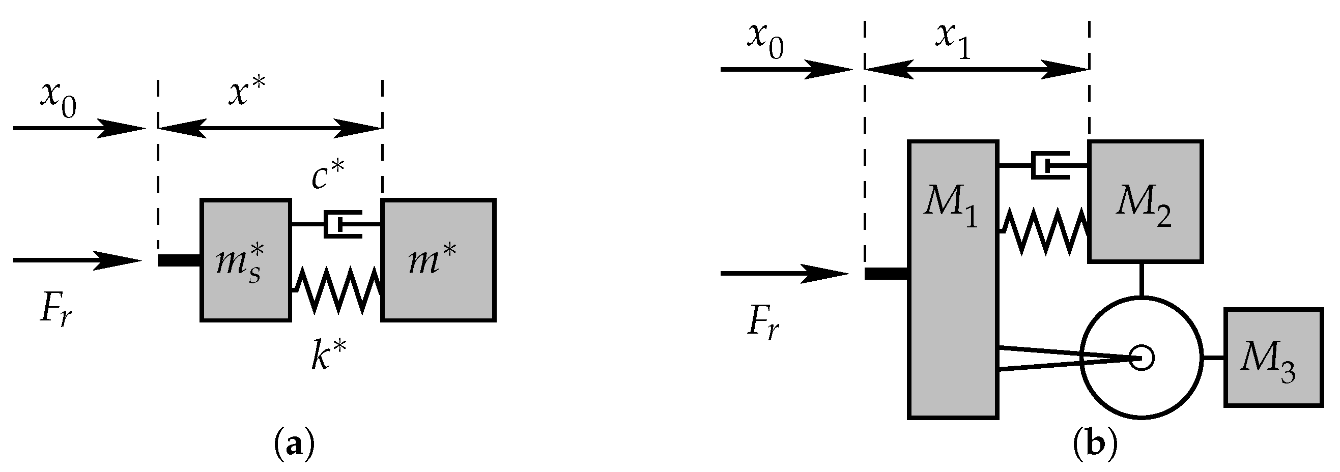
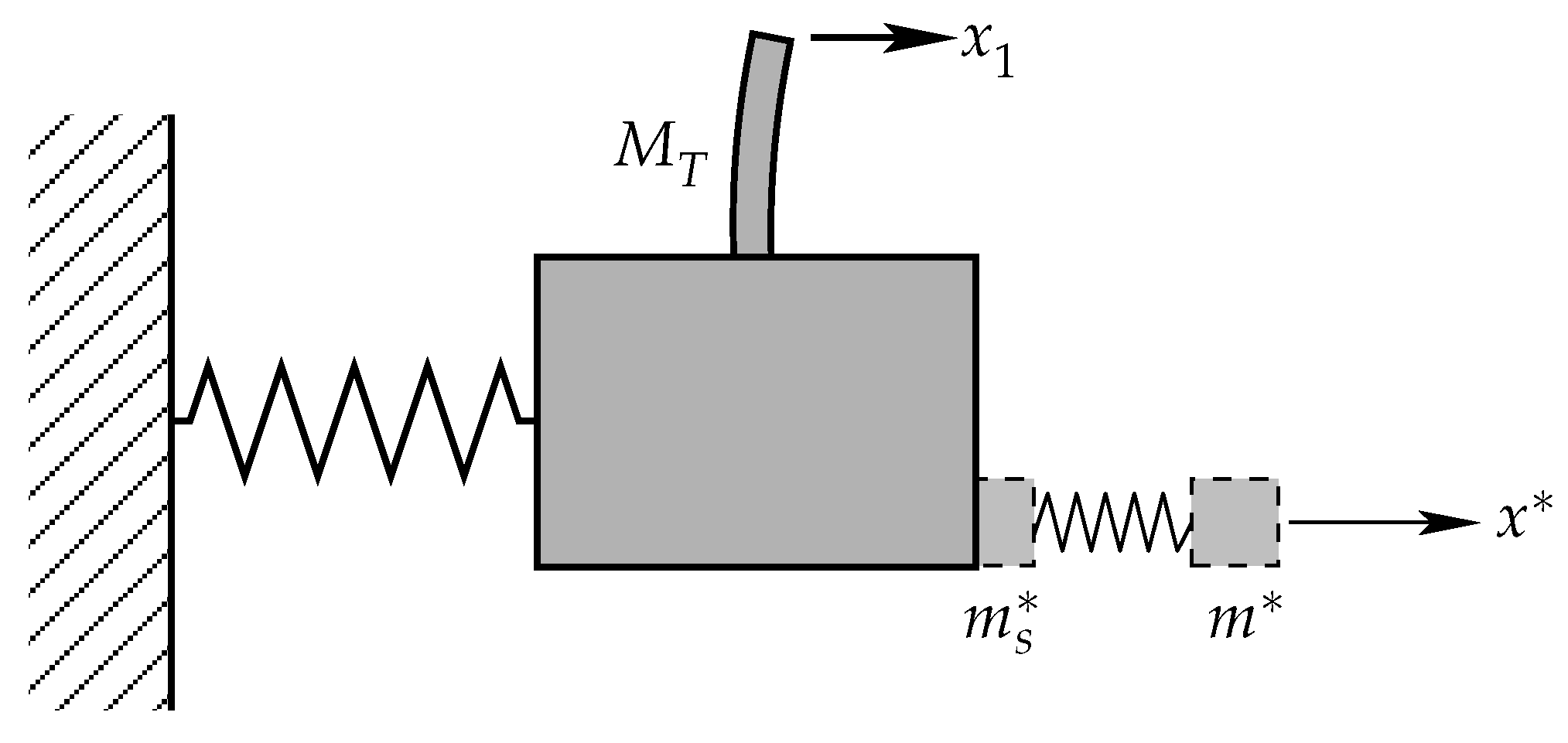
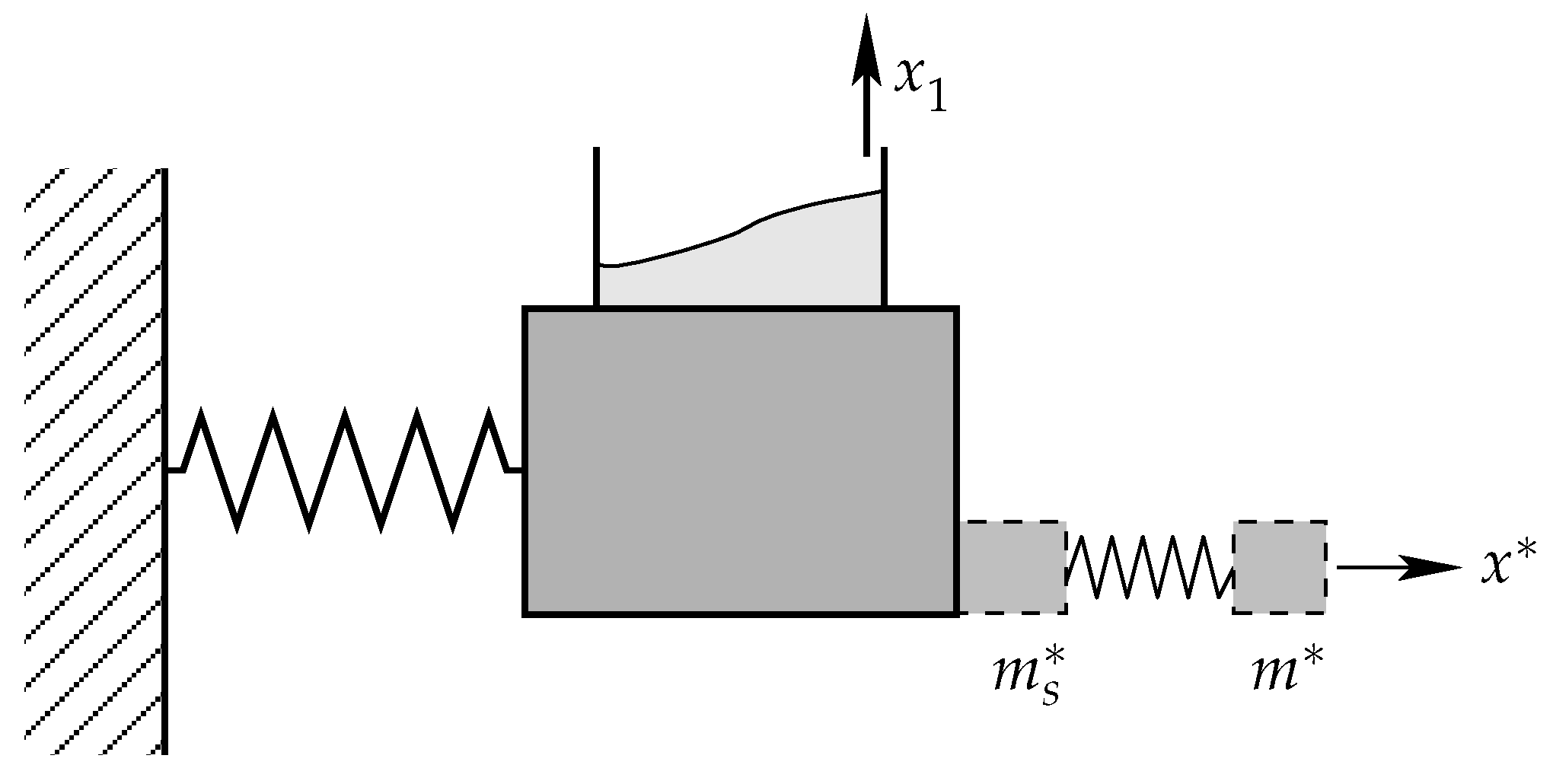
Many TMDs differ from the simple TMD by consisting of multiple mass components with motions of different magnitudes and directions. Below, a general TMD will refer to a general linear one degree-of-freedom system attached to a structure in order to provide damping. A general TMD, which is not a simple TMD, will be said to contain added mass. An example is shown in Figure 2b. Examples also include wave dampers (also called liquid sloshing dampers), tuned liquid column dampers and pendulum dampers. Come to think of it, any TMD in fact contains some added mass, because springs and wires have non-zero mass.

Added mass changes the TMD dynamics in a way that is often not well understood. In particular, the mass of a general TMD can be described in several ways, including the inertial mass $M_I$ associated with the momentum of the damper in the direction of the structure motion, the kinetic energy mass $M_K$ (sometimes referred to as the modal mass) associated with the kinetic energy internal to the damper and the total mass $M_T$ equal to the sum of the masses of each damper component (see also Section 3.3). The masses $M_I$ and $M_K$ are not uniquely defined, because they depend on the arbitrary choice of scaling of the internal TMD motions. Which, if any, of these three masses should be taken as the effective TMD mass?

This question is addressed in this paper, where we develop a framework for determining parameters for the equivalent simple TMD for a given general TMD. The ambiguity of the TMD mass and amplitude of motion are removed, and the effective TMD mass, denoted $m^{*}$, is defined in terms of the above-mentioned masses $M_I$ and $M_K$. It is shown that added mass in fact reduces the effective TMD mass. When designing a TMD with significant added mass, it is therefore imperative to understand its effect in order to assess the TMD effectiveness correctly and in order to properly tune the TMD.

The concept of an effective mass is known in several contexts, but to the knowledge of the authors, it has not been formulated as a general concept for TMDs. The same concept is used in earthquake engineering; see Section 13.2.2 in [21], where the effective mass is termed the “base shear effective modal mass”. Discussions of the equivalent system also arise in the literature on spacecraft dynamics, e.g., [22], where it is termed the “equivalent spring-mass system”; in the literature on liquid sloshing dynamics, see [23] and the references herein, e.g., [24], and in the literature on TLCDs, see [25]. In [21] and [22], the effective mass was treated in terms of modal analysis, and it was noted in [21] that the full modal spectrum may be regarded as a set of effective masses, which sum up to the total mass. In [23], equivalent parameters were deduced from a full computation of the pressure-induced forces on the walls of a liquid container. In [25,26], the “active mass” of a TLCD was computed by solving the dynamical equations particular to a TLCD. The results from [25,26] were used in the SYNPEX guidelines [27], which unfortunately include the dangerously misleading statement that “The TLCD can be designed with lower mass ratios and still perform as well as a TMD with higher mass”, where in fact, the TLCD is equivalent to a simple TMD with lower mass. The concept of effective mass is difficult and surrounded by misunderstandings in the engineering community.

The current paper takes a different approach. The equivalent system parameters are deduced for a system with a single prescribed mode shape. The theory is developed from first principles in a self-contained derivation. The resulting framework is simple and easy to use in the context of TMDs. A number of examples are given in Section 5, where complicated calculations found in the literature are reproduced by a simple application of the framework developed here.

Guide to the Reader

The theory presented in this paper is simple and only relies on elementary mathematics. However, there is still ample possibility for confusion. In particular, it is important to separate the different systems being discussed:

• A simple TMD denotes a Tuned Mass Damper (TMD), where all mass moves in the same direction of the main structure. The simple TMD is characterized by the following parameters: m, $m_s^{}$, $\omega$, $\zeta$ and the coordinate of internal motion $x_1^{}$. See Section 2 and Figure 1.
• A general TMD denotes a general linear one degree-of-freedom system attached to a moving structure and consisting of N mass elements, whose motion relative to the structure is governed by a single coordinate $x_1^{}$. The general TMD is governed by the parameters $\omega$ and $\zeta$ and by three measures of the mass $M_T^{}$, $M_I^{}$ and $M_K^{}$. If $M_K^{}\ne M_I^{}$, the TMD is considered to contain added mass. See Section 3.3.
• An equivalent simple TMD denotes a simple TMD (see above), which is dynamically equivalent to a given general TMD (see below). The equivalent simple TMD is characterized by the parameters $m_{}^{*}$ (the effective TMD mass), $m_s^{*}$, $\omega$ and $\zeta$, where the asterisk (*) emphasizes derived equivalent parameters. See Section 3.

The reader is encouraged to refer back to these definitions while reading below. If an example is desired, the reader may begin by reading the example in Section 5.1 before tackling Section 3 and Section 4.

The paper is organized as follows. Section 2 describes the operation of a simple TMD and emphasizes the role of the reaction force exerted by the TMD on the main structure. Section 3 investigates the reaction force for both a simple TMD and a general TMD and derives expressions for equivalent simple TMD parameters for a given general TMD. The parameters are investigated in the context of the full system in Section 4. Section 5 applies the developed framework to a number of systems, including numerical examples. Finally, Section 6 gives a short summary.

2. Tuned Mass Damper Principle of Operation

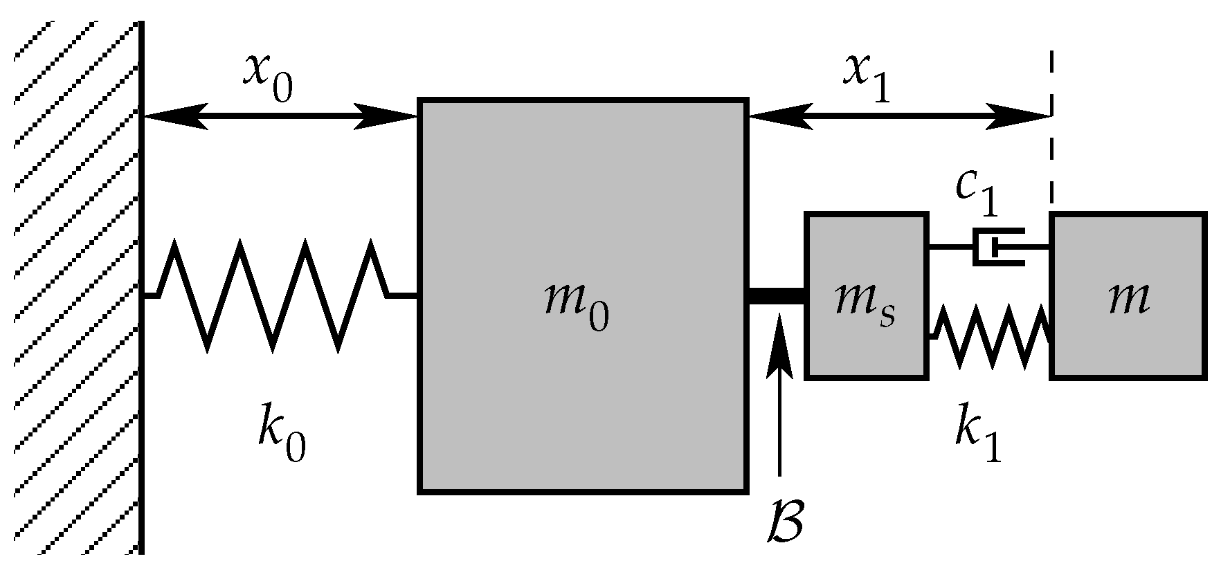
A TMD is a local device put on a structure with the aim of affecting the vibrations of the structure. An example of a TMD in its simplest form (below, referred to as a simple TMD) is shown in Figure 1. All components are considered restricted to move in the horizontal direction. We shall denote time by t and differentiation with respect to time by a dot, $\dot{x}\equiv \frac{\partial x}{\partial t}$.

A structure of mass $m_0$ is attached to an inertial frame by a spring of rate $k_0$. On the structure, the TMD is attached by a rigid bar $\mathcal{B}$. The TMD consists of a mass $m_s$ fixed to $m_0$ by the rigid bar and a mass m, which is connected to $m_s$ by a spring of rate $k_1\equiv m{\omega }^2$, as well as a linear damper of rate $c_1\equiv 2m\omega \zeta$. Here, we have introduced the TMD internal frequency $\omega$ and the TMD internal damping ratio $\zeta$, which can be measured by holding the structure fixed $x_0^{}\left(t\right)=0$ and performing a decay test on the TMD. The coordinates of the system are the absolute position $x_0$ of the structure and the position $x_1$ of m relative to the structure. The TMD affects the motion of $m_0$ by imposing a reaction force $F_r$ on $m_0$. Referring to Figure 1, $F_r$ is defined as the tensile force acting through $\mathcal{B}$.

Note that the structure-fixed mass $m_s$, e.g., the bolts holding the TMD in place on the structure, is traditionally either disregarded entirely or simply counted as part of the structure mass. For the present discussion, it is however useful to identify $m_s$ explicitly.

Below, we shall investigate the reaction force for the simple TMD sketched in Figure 1 and for more complex TMD systems.

3. Reaction Force for General Linear One Degree-of-Freedom Oscillators

Figure 2 shows two different TMD configurations. Comparing to Figure 1, everything to the right of $\mathcal{B}$ is shown. Figure 2a shows a simple TMD, and Figure 2b shows an example of a general TMD, including added mass. It will be shown below that a general linear one degree-of-freedom oscillator can be described as an equivalent simple system as shown in Figure 2a by choosing appropriate equivalent parameters $m_s^{*}$, $m_{}^{*}$, $c_{}^{*}$ and $k_{}^{*}$.

3.1. Simple TMD

For the simple TMD shown in Figure 2a, the reaction force $F_r=F_r\left(t\right)$ and the equation of motion governing $x^{*}=x^{*}\left(t\right)$ are determined directly from momentum conservation:

$$\begin{array}{c}\hfill F_r=-m_s^{*}{\ddot{x}}_0-m^{*}({\ddot{x}}_0+{\ddot{x}}^{*}),\end{array}$$

(1)

$$\begin{array}{c}\hfill {\ddot{x}}^{*}+{\ddot{x}}_0+2\zeta \omega {\dot{x}}^{*}+{\omega }^2{x}^{*}=0,\end{array}$$

(2)

where we have written Equation (2) in terms of ${\omega }^2\equiv \frac{k^{*}}{m^{*}}$ and $\zeta \equiv \frac{c^{*}}{2m^{*}{\omega }^{*}}$.

3.2. Example of a Complex General TMD

Consider the example of a complex general TMD sketched in Figure 2b. The TMD consists of several mass components. The mass $M_1$ is fixed to the structure. The masses $M_2$ and $M_3$ are connected through a massless wheel, such that they both move according to the coordinate $x_1$, but $M_2$ moves parallel to $x_0$ and $M_3$ moves perpendicular to $x_0$.

We look for an equivalent simple TMD of the type shown in Figure 2a. The equivalent simple TMD parameters are determined from the parameters of the general TMD. We are especially interested in the effective TMD mass $m_{}^{*}$. The mass $M_3$ is an example of added mass. It makes it harder to turn the wheel, effectively restricting the motion of $M_2$. We now use a heuristic argument to illustrate how the magnitude of $M_3$ affects $m_{}^{*}$.

• Consider first the case $M_3=0$. Then, the equivalence is trivial with $m_{}^{*}=M_2$ and $m_s^{*}=M_1$.
• We now hold $M_2$ fixed and increase $M_3$, until $M_3\gg M_2$. Then, the wheel is effectively prevented from moving, and the entire TMD acts as a rigid mass, so $m_{}^{*}\approx 0$ and $m_s^{*}\approx M_1+M_2+M_3$.
• For intermediate values of $M_3$, the movement of $M_2$ will be somewhat reduced compared to Case 1, giving an effective TMD mass $0<m_{}^{*}<M_2$.

The above argument shows that the presence of $M_3$ may reduce the effective TMD mass $m_{}^{*}$. Below, we replace the heuristic argument with a quantitative analysis. This will be done for a completely general linear one degree-of-freedom TMD (denoted a general TMD).

3.3. Analysis of a General TMD

We now consider a general TMD. The TMD shown in Figure 2 is one example, but in general, the TMD may consist of any number of mass components, each constrained to move in a coordinated manner according to a single coordinate $x_1$. The system is attached to a moving base, with a position described as $x=x_0\left(t\right)$ in an orthogonal $(x,y,z)$-coordinate system. As in Section 3.1, we wish to know the reaction force in the x-direction onto the base and the equation of motion governing $x_1\left(t\right)$.

Consider N mass elements named $M_i$ with $i=1,\dots ,N$. The motion of all elements is given by a single coordinate $x_1$, and a spring and dashpot act on the system to introduce stiffness and damping. The potential energy of the system is $V=\frac{1}{2}{k}_1{x}_1^2$, and the Rayleigh damping functional is $\mathcal{F}=\frac{1}{2}{c}_1^{}{\dot{x}}_1^2$. We parameterize the motion of $M_i$ by the vector $({\rho }_i,{\sigma }_i,{\tau }_i)$, such that the absolute position of $M_i$ is $(x,y,z)=(x_0,0,0)+x_1({\rho }_i,{\sigma }_i,{\tau }_i)$, where $({\rho }_i,{\sigma }_i,{\tau }_i)$ are constants. We first introduce the following shorthand notation:

$$\begin{array}{ccc}\mathrm{the}\mathrm{total}\mathrm{mass}:\hfill & \hfill M_T^{}& {\displaystyle \equiv \sum _i{M}_i,}\hfill \end{array}$$

(3)

$$\begin{array}{ccc}\mathrm{the}\mathrm{inertial}\mathrm{mass}:\hfill & \hfill M_I^{}& {\displaystyle \equiv \sum _i{M}_i{\rho }_i,}\hfill \end{array}$$

(4)

$$\begin{array}{ccc}\mathrm{the}\mathrm{kinetic}\mathrm{energy}\mathrm{mass}:\hfill & \hfill M_K^{}& {\displaystyle \equiv \sum _i{M}_i({\rho }_i^2+{\sigma }_i^2+{\tau }_i^2).}\hfill \end{array}$$

(5)

The masses defined in Equations (3)–(5) characterize the TMD. A simple TMD corresponds to a mode shape with motion only in the x-direction, ${\sigma }_i={\tau }_i=0$ and ${\rho }_i$ taking only the values zero and one, leading to $M_I^{}=M_K^{}$. For any other mode shape, we will have $M_I^{}\ne M_K^{}$. A general TMD with $M_I^{}\ne M_K^{}$ will be referred to as having added mass.

The mass $M_K^{}$, Equation (5), is identical to the traditional modal mass associated with the mode shape defined by the set of vectors $({\rho }_i,{\sigma }_i,{\tau }_i)$. The masses defined in Equations (4) and (5) are not unique and depend on the choice of scaling of the coordinate $x_1$. A different choice $x_1\to {\chi }^{-1}{x}_1$ leads to $({\rho }_i,{\sigma }_i,{\tau }_i)\to \chi ({\rho }_i,{\sigma }_i,{\tau }_i)$ and to $M_I^{}\to \chi M_I^{}$ and $M_K^{}\to {\chi }^2{M}_K^{}$.

The kinetic energy of the TMD components is now:

$$\begin{array}{cc}\hfill T& =\frac{1}{2}\sum _i{M}_i^{}\left[{({\dot{x}}_0^{}+{\rho }_i^{}{\dot{x}}_1^{})}^2+{\left({\sigma }_i{\dot{x}}_1^{}\right)}^2+{\left({\tau }_i{\dot{x}}_1^{}\right)}^2\right]\hfill \\ & =\frac{1}{2}\sum _i{M}_i^{}\left[{\dot{x}}_0^2+2{\rho }_i{\dot{x}}_0^{}{\dot{x}}_1^{}+({\rho }_i^2+{\sigma }_i^2+{\tau }_i^2){\dot{x}}_1^2\right]\hfill \\ & =\frac{1}{2}{M}_T^{}{\dot{x}}_0^2+M_I^{}{\dot{x}}_0^{}{\dot{x}}_1^{}+\frac{1}{2}{M}_K^{}{\dot{x}}_1^2.\hfill \end{array}$$

(6)

The Lagrangian of the system is $L\equiv T-V$. The reaction force $F_r$ against the motion $x_0$ is obtained as $F_r=-\frac{\partial L}{\partial x_0}$. The equation of motion governing $x_1$ is found by the Euler–Lagrange equation $\frac{\mathrm{d}}{\mathrm{d}t}\left(\frac{\partial L}{\partial {\dot{x}}_1}\right)-\frac{\partial L}{\partial x_1}=-\frac{\partial \mathcal{F}}{\partial {\dot{x}}_1}$. We get:

$$\begin{array}{cc}\hfill F_r& =-M_T^{}{\ddot{x}}_0-M_I^{}{\ddot{x}}_1,\hfill \end{array}$$

(7)

$$\begin{array}{cc}\hfill 0& ={\ddot{x}}_1+\frac{M_I^{}}{M_K^{}}{\ddot{x}}_0+2\zeta \omega {\dot{x}}_1+{\omega }^2{x}_1,\hfill \end{array}$$

(8)

where we have introduced the TMD internal angular frequency $\omega$ and damping ratio $\zeta$,

$$\begin{array}{cc}\hfill \omega & \equiv \sqrt{\frac{k_1^{}}{M_K^{}}},\hfill \end{array}$$

(9)

$$\begin{array}{cc}\hfill \zeta & \equiv \frac{c_1^{}}{2M_K^{}\omega }\hfill \end{array}$$

(10)

The equivalent frequency and damping ratio given by Equations (9)–(10) are those that would be observed by keeping the base stationary $x_0\left(t\right)=0$ and performing a decay test on the TMD. We exclude from our attention the case $M_I^{}=0$, which would leave the TMD dynamically uncoupled from the main structure; see Equation (8).

Now, Equations (7)–(8) are rather similar to Equations (1)–(2), except that in Equation (8), the coefficients ${\ddot{x}}_1$ and ${\ddot{x}}_0$ are of different magnitude. We can however find a set of equivalent simple TMD parameters, $m_s^{*}$, $m^{*}$ and $x^{*}$, that bring Equations (1)–(2) into the form of Equations (7)–(8). This can be done in an elementary way. We start from Equation (2) and derive the substitutions given below in Equations (11)–(13) as follows: In order to match the first two terms in Equation (8), we substitute $\frac{M_K}{M_I}{x}_1$ for $x^{*}$ and multiply on both sides by $\frac{M_I^{}}{M_K^{}}$. Returning to Equation (1), we substitute $\frac{M_K}{M_I}{x}_1$ for $x^{*}$ and determine $m^{*}$ and $m_s^{*}$, such that the coefficients ${\ddot{x}}_0$ and ${\ddot{x}}_1$ match Equation (7). The equivalent simple TMD parameters are:

$$\begin{array}{cc}\hfill x^{*}& \equiv {\displaystyle \frac{M_K^{}}{M_I^{}}}{x}_1^{},\hfill \end{array}$$

(11)

$$\begin{array}{cc}\hfill m^{*}& \equiv {\displaystyle \frac{M_I^2}{M_K^{}}},\hfill \end{array}$$

(12)

$$\begin{array}{cc}\hfill m_s^{*}& \equiv M_T^{}-m^{*}.\hfill \end{array}$$

(13)

The simple TMD, Equations (1)–(2), with parameters chosen according to Equations (11)–(13) is thus equivalent to the general TMD, Equations (7)–(8). It will in other words generate exactly the same reaction force $F_r$ for a given motion $x_0\left(t\right)$. Note that Equations (11)–(13) uniquely defines both the amplitude of the motion, Equation (11), and the mass $m_{}^{*}$, Equation (12), which will be denoted as the effective TMD mass. The ambiguity of the masses defined in Equations (3)–(5) is thus removed.

The parameters in Equations (11)–(13) show us the following: The motion of the equivalent simple TMD is scaled relative to the motion of the general TMD. The general TMD of total mass $M_T$ acts like an equivalent simple TMD of a smaller mass $m_{}^{*}\le M_T$, Note that $m^{*}\le M_T$ is assured for any mass distribution $M_i$ and motion $({\rho }_i,{\sigma }_i,{\tau }_i)$. This is shown by noting that $M_i>0$, that the function $f(a,b)={\sum }_i{M}_i{a}_i{b}_i$ forms an inner product and using the Cauchy–Schwarz inequality to obtain $\left({\sum }_i{M}_i\right)\left({\sum }_i{M}_i{\rho }_i^2\right)\ge {\left({\sum }_i{M}_i{\rho }_i\right)}^2$, from which the result follows. The remainder of the mass of the complex system $m_s^{*}$ is effectively added to the structure. Since $m^{*}=M_T$ for a simple TMD, i.e., a TMD with ${\rho }_i=1$, ${\sigma }_i={\tau }_i=0$, we conclude that out of all general TMDs with a given total mass $M_T$, the simple TMD gives the highest possible effective TMD mass $m^{*}$.

4. Application to a Structure with a General TMD

We have seen above in Section 3 that a general TMD may be described as an equivalent simple TMD. In order to describe the combined action of the main structure $m_0$ and the TMD (see Figure 1), we introduce the effective mass ratio ${\mu }^{*}$ and the effective structure angular frequency ${\omega }_0^{*}$. Their expressions follow directly from considering the effective TMD mass as $m^{*}$ and the effective structure mass as $m_0+m_s^{*}$:

$$\begin{array}{cc}\hfill {\mu }^{*}& =\frac{m^{*}}{m_0+m_s^{*}},\hfill \end{array}$$

(14)

$$\begin{array}{cc}\hfill {\omega }_0^{*}& =\sqrt{\frac{k_0}{m_0+m_s^{*}}}=\frac{{\omega }_0^{}}{\sqrt{1+\frac{m_s^{*}}{m_0}}},\hfill \end{array}$$

(15)

where ${\omega }_0^{}=\sqrt{\frac{k_0}{m_0}}$ is the frequency of the isolated structure.

Using the results of Section 3, in particular Equations (11)–(13), the tuning of a general TMD can be done based on the classical tuning rules found in the literature. Classical optimum tuning for harmonic forcing [2] involves choosing optimal parameters ${\omega }_{\mathrm{opt}.}^{}=\frac{1}{1+\mu }{\omega }_0$ and ${\zeta }_{1,\mathrm{opt}.}^2=\frac{3}{8}\frac{\mu }{1+\mu }$. For a general TMD, this becomes:

$$\begin{array}{cc}\hfill {\omega }_{\mathrm{opt}.}^{}& =\frac{1}{1+{\mu }^{*}}{\omega }_0^{*},\hfill \end{array}$$

(16)

$$\begin{array}{cc}\hfill {\zeta }_{\mathrm{opt}.}^{}& =\sqrt{\frac{3}{8}\frac{{\mu }^{*}}{1+{\mu }^{*}}},\hfill \end{array}$$

(17)

As we saw in Section 3, the effective mass ratio, Equations (14)–(15), is generally smaller than the naive mass ratio ${\mu }_{\mathrm{naive}}=\frac{M_T}{m_0}$, so an optimal general TMD with added mass $M_K\ne M_I$ has a tuning closer to the structure natural frequency than a simple TMD with $m^{}=M_T^{}$. Furthermore, the internal damping ${\zeta }_{\mathrm{opt}.}^{}$ is lower than that for a simple TMD with $m^{}=M_T^{}$. For random white-noise forcing, a more appropriate optimum frequency is, [10],

$$\begin{array}{c}\hfill {\omega }_{\mathrm{opt}.\text{white-n}.}^{}=\frac{\sqrt{1+\frac{1}{2}{\mu }_{}^{*}}}{1+{\mu }_{}^{*}}{\omega }_0^{*}.\end{array}$$

(18)

5. Examples of TMDs with Added Mass

The following sections show nine different examples of general TMD systems where added mass influences the TMD efficiency. The framework developed above is used to determine the parameters of an equivalent simple TMD, including the effective TMD mass. In some of the examples, optimal tuning parameters are also discussed based on the equivalent simple TMD parameters. Where relevant, the results in the examples have been compared to the literature; see Section 5.2, Section 5.4, Section 5.5, Section 5.6 and Section 5.7. This comparison serves to illustrate how complicated calculations on a particular TMD example can be replaced by simple computation based on the framework developed above. The comparison also serves as a confirmation of the developed framework. The examples include simple mechanical systems, as well as fluid dynamic systems. The examples illustrate that the effective TMD mass may be much lower than one might expect from a naive estimate; see in particular Section 5.2 and Section 5.5.

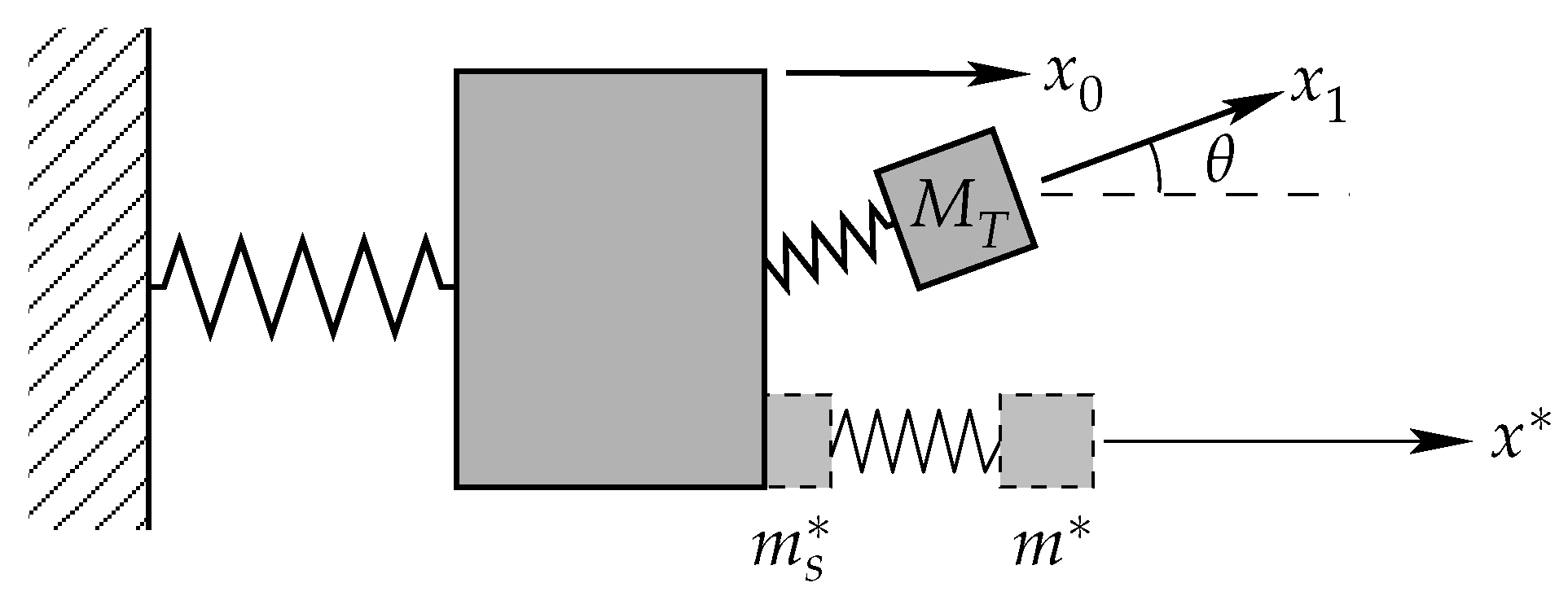
5.1. Misaligned TMD

Consider a TMD consisting of a simple mass-on-a-spring with a mass $M_T^{}$, whose direction of motion differs by an angle $\theta$ from the direction of motion of the main structure, as sketched in Figure 3. Such a misalignment may easily arise by inaccurate construction or placement of a TMD or by a misinterpretation of the main structure mode shape.

How can we assess the effective TMD mass $m_{}^{*}$? Clearly, $m_{}^{*}<M_T^{}$. A naive estimate of the effective TMD mass would be $M_T^{}cos\theta$, because the action of the inertial force from the TMD along $x_0$ is reduced by a factor $cos\theta$ due to the misalignment. This estimate is wrong, however, because it disregards the fact that the inertial forces due to the structure motions, which set the TMD in motion in the first place, are also reduced by a factor of $cos\theta$. Due to this double effect of the misalignment, we therefore speculate that the effective TMD mass is $m_{}^{*}=M_T^{}{cos}^2\theta$.

The question can be resolved by consulting the framework developed in Section 3. The momentum in the direction of $x_0$ is $M_I^{}{\dot{x}}_1$, where the inertial mass is defined as $M_I^{}=M_T^{}cos\theta$. The kinetic energy internal to the TMD is $\frac{1}{2}{M}_K^{}{\dot{x}}_1^2$, where the kinetic energy mass is defined as $M_K^{}=M_T$. We see from Section 3 and Equations (11)–(13) that the misaligned TMD behaves as an equivalent simple TMD with the effective TMD mass $m_{}^{*}=\frac{M_I^2}{M_K}=M_T^{}{cos}^2\theta$ and motion amplitude $x^{*}=\frac{x_1}{cos\theta }$ and that the remaining mass $m_s^{*}=M_T^{}-m_{}^{*}$ is effectively fixed to the structure.

5.2. TMD with Simple Added Mass (the Example from Section 3)

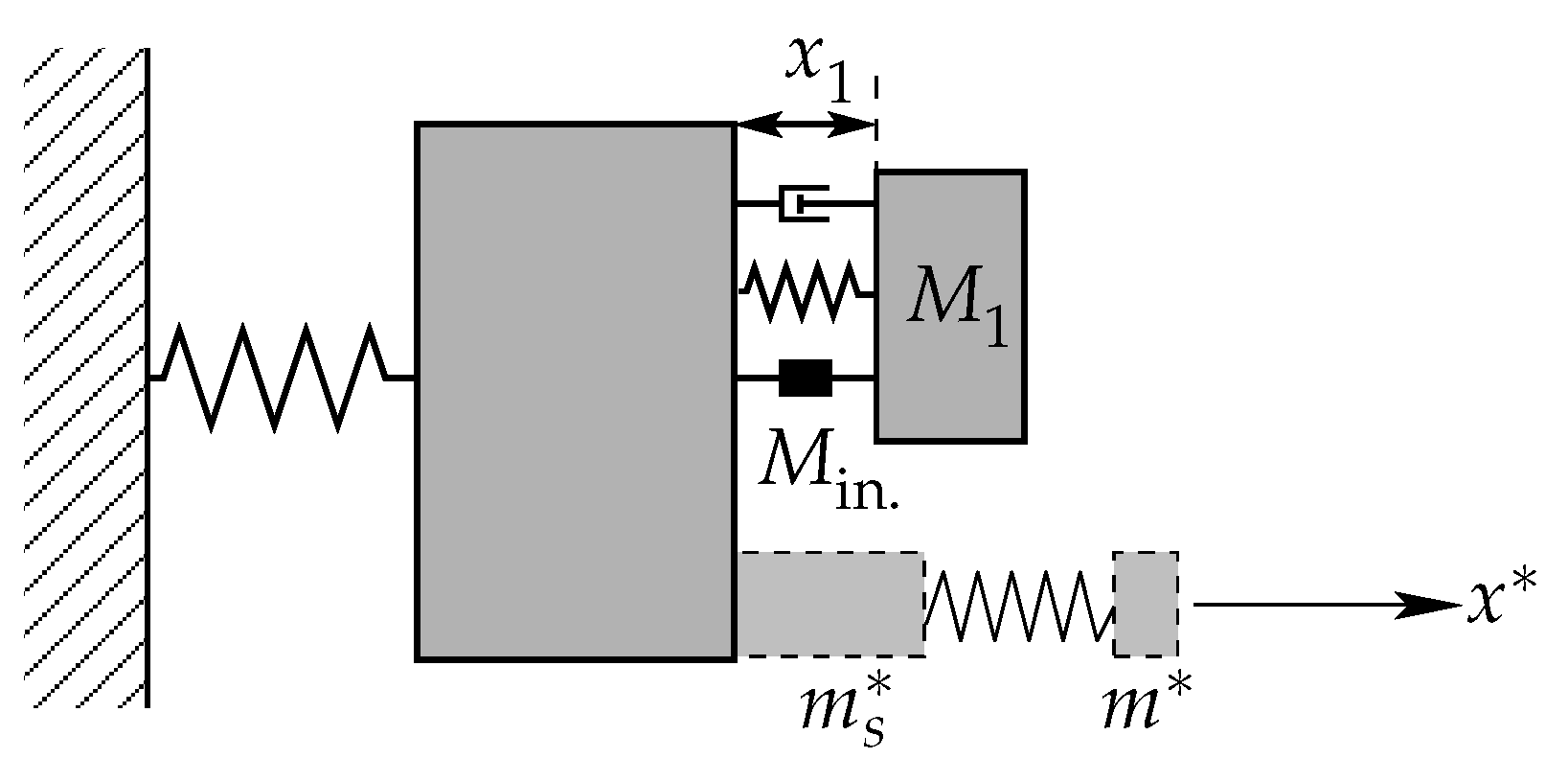
Consider the example shown in Figure 2b. There are $N=3$ TMD components with $({\rho }_1,{\sigma }_1,{\tau }_1)=(0,0,0)$, $({\rho }_2,{\sigma }_2,{\tau }_2)=(1,0,0)$, $({\rho }_3,{\sigma }_3,{\tau }_3)=(0,1,0)$. From Equations (3)–(5), we then get $M_T=M_1+M_2+M_3$, $M_I=M_2$, $M_K=M_2+M_3$, and from Equations (11)–(13), we get $m_{}^{*}=\frac{M_2^2}{M_2^{}+M_3^{}}$ and $m_s^{*}=M_1+\frac{M_2{M}_3}{M_2+M_3}+M_3$. If the TMD is attached to a structure of mass $m_0$, we use Equations (14)–(15) to get the effective mass ratio ${\mu }^{*}=\frac{M_2^2}{M_2+M_3}/\left(m_0+M_1+\frac{M_2{M}_3}{M_2+M_3}+M_3\right)$.

Consider now as an example $M_1=0.5\mathrm{kg}$, $M_2=M_3=8\mathrm{kg}$, $m_0=80\mathrm{kg}$. The above results show that the equivalent simple TMD mass is $m_{}^{*}=4\mathrm{kg}$, and $m_s^{*}=12.5\mathrm{kg}$. The effective mass ratio is now ${\mu }^{*}=\frac{4\mathrm{kg}}{92.5\mathrm{kg}}=4.3\%$. Note how in this example, the “passive” mass $m_s^{*}$ is considerably larger than the combined masses $M_1$ and $M_3$. Using the classical optimal tuning rule, Equation (16), we get ${\omega }_{\mathrm{opt}}^{}.=\frac{1}{1+4.3\%}\sqrt{\frac{80}{92.5}}{\omega }_0=0.891{\omega }_0$.

We remark that if one had used the naive assumption ${m_{}^{*}}^{\prime }=8\mathrm{kg}$, the mass ratio would erroneously be interpreted as ${\mu }^{\prime }=\frac{8}{88.5}=9.0\%$ and the optimal tuning frequency as ${{\omega }_{\mathrm{opt}}^{}.}^{\prime }=\frac{1}{1+9.0\%}\sqrt{\frac{80}{88.5}}{\omega }_0=0.872{\omega }_0$. This example shows how the naive interpretation of the effect of added mass can lead to significant errors in the interpretation of the effective TMD mass, the effective mass ratio and the optimal tuning frequency. In the present case, a TMD design based on the naive interpretation would have an effective mass less than half the expected value. It would perform dramatically worse than expected and furthermore be tuned significantly away from its optimum.

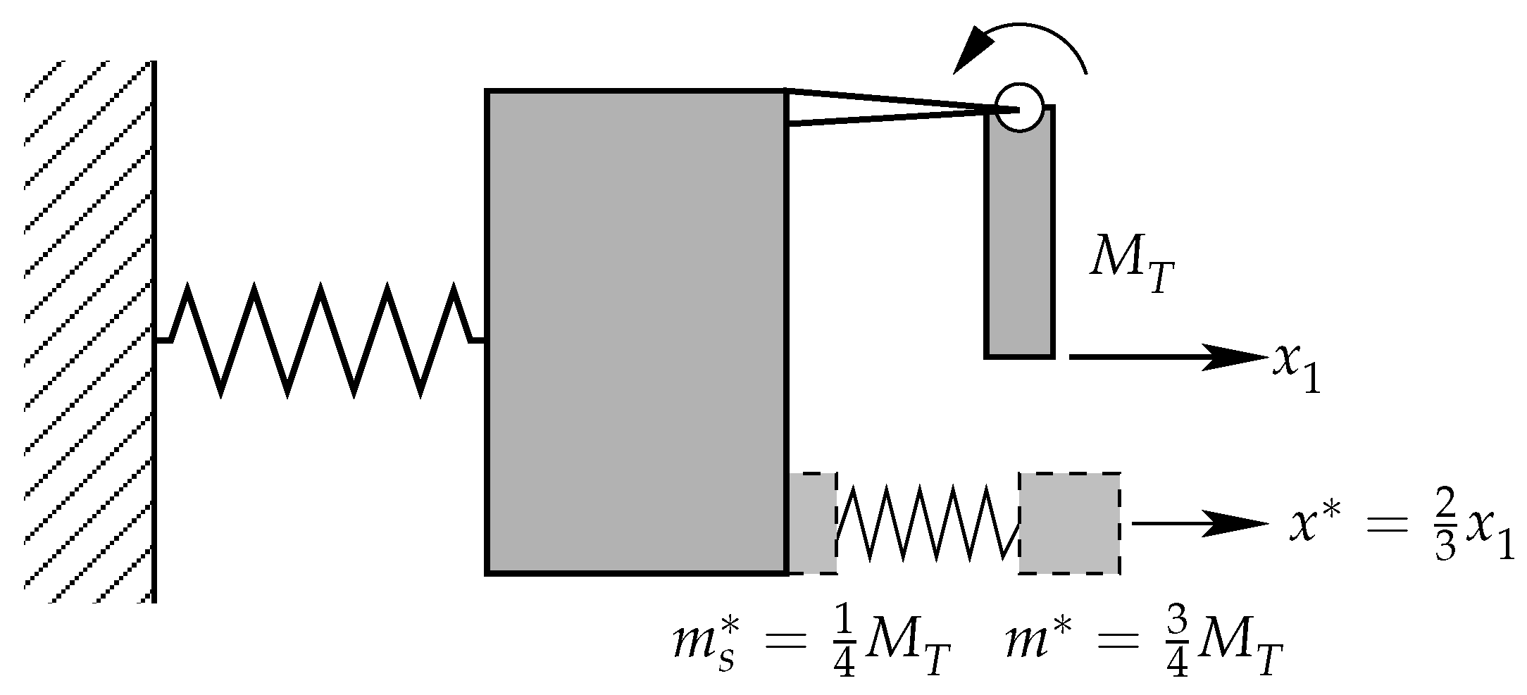
5.3. Uniform Beam Pendulum

Consider a rigid uniform beam pendulum of total mass $M_T$, as shown in Figure 4. We consider small displacements and linearize the motions. Parameterizing the pendulum length by $0\le q\le 1$, the displacements are $\rho \left(q\right)=q$ and $\sigma \left(q\right)=\tau \left(q\right)=0$. Now that the TMD mass components are continuously indexed, the sums in Equations (3)–(5) are replaced with integrals, and we get $M_I=M_T{\int }_0^{1}q\mathrm{d}q=\frac{1}{2}{M}_T$ and the kinetic energy mass $M_K=M_T{\int }_0^1{q}^2\mathrm{d}q=\frac{1}{3}{M}_T$. The effective TMD mass, Equations (11)–(13), is therefore:

$$\begin{array}{c}\hfill m_{}^{*}=\frac{3}{4}{M}_T,m_s^{*}=\frac{1}{4}{M}_T.\end{array}$$

(19)

From Equations (11)–(13), we get $x^{*}=\frac{2}{3}{x}_1$. The pendulum is therefore equivalent to a simple TMD of mass $\frac{3}{4}{M}_T$ with a deflection equal to that of the two-thirds point on the pendulum; see Figure 4.

5.4. Uniform Cantilever Beam TMD

Consider a uniform cantilever beam of total mass $M_T$ acting as a TMD, as shown in Figure 5. The beam is considered slender and clamped to the main structure, and we consider the fundamental vibration mode. This system was investigated in [28], and the optimal tuning ratio was determined. The deflection as a function of the normalized distance from the fixed end $u\in [0,1]$ is, cf. [29], Table 8-1(3),

$$\begin{array}{c}\hfill \rho \left(u\right)=cosh\nu -cos\nu -0.734(sinh\nu -sin\nu ),\end{array}$$

(20)

with $\nu \equiv 1.875u$ and $\sigma =\tau =0$. From Equations (3)–(5), $M_I^{}=M_T^{}{\int }_0^1\rho \mathrm{d}u$ and $M_K^{}=M_T^{}{\int }_0^1{\rho }^2\mathrm{d}u$, and Equations (11)–(13) gives:

$$\begin{array}{c}\hfill m^{*}=0.613M_T^{},\end{array}$$

(21)

as well as $m_s^{*}=0.387M_T^{}$ and $x^{*}=1.28x_1$. Using Equations (14)–(15) and (16), we get the optimum frequency of the cantilever beam TMD,

$$\begin{array}{c}\hfill {\omega }_{\mathrm{opt}.}^{}=\frac{1}{1+{\mu }^{*}}{\omega }_0^{*}=\frac{\sqrt{1+0.387\frac{M_T^{}}{m_0}}}{1+\frac{M_T^{}}{m_0}}{\omega }_0.\end{array}$$

(22)

This recovers the result, Equation (26) in [28], but with much less effort than by the method used in [28]. The calculation can be performed in the same way for higher vibration modes, giving much smaller values of $m_{}^{*}$ than found in Equation (21). On reading [21], we speculate that the sum of the effective TMD masses corresponding to each vibration mode will sum up to $M_T^{}$ or to a constant value lower than $M_T^{}$ depending on the nature of the mechanical connection between the structure and the TMD, but we have not investigated this property further.

5.5. Rectangular Tuned Liquid Damper

Consider a rectangular container partially filled with a liquid, so the gravity wave modes serve as TMDs; see Figure 6. Consider, in the $uv$-plane, the liquid volume to be confined to $-\frac{D}{2}<u<\frac{D}{2}$ and $0<v<H$, with the waves occurring on the free surface $v=H$. For convenience, we set the liquid density such that $M_T=HD$.

For the nth asymmetric standing wave mode admissible in the tank, the wavenumber $k_n$ and the velocity potential $\varphi$ can be written, see, e.g., [29],

$$\begin{array}{cc}\hfill k_n& =(2n-1)\frac{\pi }{D},\hfill \end{array}$$

(23)

$$\begin{array}{cc}\hfill {\varphi }_n(u,v)& =sin{k}_{n}u\frac{cosh{k}_{n}v}{k_{n}sinh{k}_{n}H},\hfill \end{array}$$

(24)

where the oscillation frequency must naturally satisfy the dispersion relation; see [29]. We use the divergence theorem to compute $M_I$ and $M_K$. Local mass conservation ${\nabla }^2\varphi =0$ implies $\nabla ·(u\nabla \varphi )=\nabla u·\nabla \varphi$ and ${(\nabla \varphi )}^2=\nabla ·(\varphi \nabla \varphi )$. Therefore, we have from Equations (3)–(5) and (11)–(13):

$$\begin{array}{cc}\hfill M_I^{}& ={\int }_{-\frac{D}{2}}^{\frac{D}{2}}\mathrm{d}u{\left[u\frac{\partial {\varphi }_n}{\partial v}\right]}_{v=H}=\pm \frac{2}{k_n^2},\hfill \end{array}$$

(25)

$$\begin{array}{cc}\hfill M_K^{}& ={\int }_{-\frac{D}{2}}^{\frac{D}{2}}\mathrm{d}u{\left[{\varphi }_n\frac{\partial {\varphi }_n}{\partial v}\right]}_{v=H}=\frac{D}{2k_n}coth{k}_{n}H,\hfill \end{array}$$

(26)

$$\begin{array}{cc}\hfill m_n^{*}& =\frac{M_I^2}{M_K^{}}=M_T^{}\frac{8}{{(2n-1)}^3{\pi }^3}\frac{D}{H}tanh(2n-1)\pi \frac{H}{D}.\hfill \end{array}$$

(27)

This result agrees with that of [24], which was also reproduced in [23] as Equation 5.19 (where by mistake, $n+1$ has been used in the place of n). Observe from Equations (11)–(13) that the wave height $x_1$ relates to the effective motion as $x_1=x_{}^{*}\frac{4}{(2n-1)\pi }tanh(2n-1)\pi \frac{H}{D}$.

We see from the above results that TLDs use a very limited fraction of total liquid mass. With a fixed total liquid mass $M_T^{}$, the maximal effective TMD mass occurs in the low-depth limit $\frac{H}{D}\to 0$, with Equation (27) giving $\frac{m_1^{*}}{M_T^{}}\to \frac{8}{{\pi }^2}=0.81$, $\frac{m_2^{*}}{M_T^{}}\to 0.09$, and so on. Furthermore, very shallow TLDs are impractical, because ugly non-linear effects set in for low values of $\frac{H}{D}\lesssim 0.40$. Using Equation (27), we get the corresponding ratios of the effective TMD mass to the total liquid mass $\frac{m_1^{*}}{M_T^{}}{|}_{\frac{H}{D}\gtrsim 0.40}\lesssim 0.55$ and $\frac{m_2^{*}}{M_T^{}}{|}_{\frac{H}{D}\gtrsim 0.40}\lesssim 0.02$. This corresponds to exploiting only the mass of the liquid down to a depth of $0.22D$ for $n=1$ and down to a depth of $0.01D$ for $n=2$. For large liquid depths, we see from Equation (27) that $m_1^{*}$ corresponds to the mass of the liquid down to the depth $\frac{8}{{\pi }^3}D=0.26D$ and that $m_2^{*}$ corresponds to the mass of the liquid down to the depth $\frac{8}{3^3{\pi }^2}D=0.01D$. The relation between $m_1^{*}$ and the total liquid mass is illustrated in Figure 7.

This example shows an application of the framework developed in Section 3 and demonstrates the very limited efficiency of TLDs. Consider for simplicity a TLD of horizontal tank length 1 m. At best, the fundamental mode $n=1$ effectively uses the top 26 cm of liquid as a TMD, while the second mode only effectively uses the upper 1 cm of liquid as a TMD.

5.6. Cylindrical TLD

We briefly state the results corresponding to the previous section for a cylindrical TLD of liquid depth H and tank diameter D, using the flow potential given in [23]. The results for the fundamental wave mode are $\frac{m_1^{*}}{M_T^{}}{|}_{\frac{H}{D}\to 0}=0.84$, $\frac{m_1^{*}}{M_T^{}}{|}_{\frac{H}{D}=0.40}=0.51$ and $m_1^{*}{|}_{\frac{H}{D}\to \infty }=0.23\frac{M_T}{H}$, in agreement with [23].

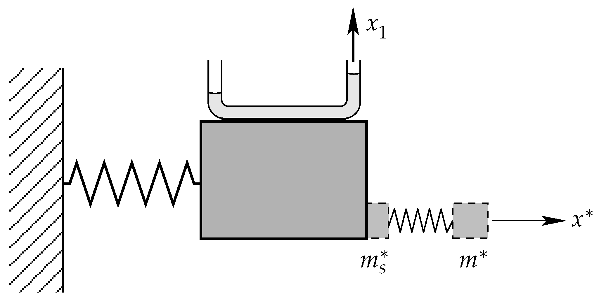
5.7. Tuned Liquid Column Damper

Consider a TLCD as shown in Figure 8. The liquid of mass $M_T^{}$ is contained in a tube of total length b and horizontal length a. We denote $\alpha \equiv \frac{a}{b}$. From local mass conservation, we observe that $M_I^{}=\alpha M_T^{}$ and $M_K^{}=M_T$. From Equations (11)–(13), we then get $m^{*}={\alpha }^2{M}_T$, $x_s^{*}=(1-{\alpha }^2)M_T$ and $x^{*}={\alpha }^{-1}{x}_1$. Note that (as for any TMD with added mass) the effective TMD mass is reduced by the presence of added mass, with $m_{}^{*}<\alpha M_T^{}<M_T^{}$. The effective mass ratio, Equations (14)–(15), is now ${\mu }^{*}=\frac{{\alpha }^2{M}_T}{m_0+M_T(1-{\alpha }^2)}$, and the optimal tuning follows directly from Equation (16) or Equation (18).

This system was studied in [25,26,30], but we can reproduce those results with much less effort. Using the above, the optimal tuning result of [30,31] (Equation (7b) in [30]) for white noise excitation is exactly recovered from the classical TMD result, Equation (18). Similarly, the effective mass ratio in [25,26] is reproduced by Equations (14)–(15). Whereas the references solve the dynamical equations governing the particular system (TLCD), the above results follow as a simple application of the general theory developed above.

5.8. Liquid-Immersed TMD

Consider a solid block immersed in an incompressible liquid, as sketched in Figure 9. The liquid could have bee introduced for the purpose of introducing damping or for lowering the TMD frequency. The solid block mass is $M_1$. The displaced liquid mass, i.e. the liquid mass density times the volume of the steel block, is $M_D$. To the motion of the steel block is associated a hydrodynamic mass $M_H^{}$, which is of order $M_D$; see, e.g., Blevins [29]. We now have $M_K^{}=M_1^{}+M_H^{}$ and, due to local mass conservation, $M_I^{}=M_1-M_D$. From Equations (11)–(13), the effective TMD mass is $m^{*}=\frac{{(M_1^{}-M_D^{})}^2}{M_1+M_H}<M_1$.

Typically, for this situation, $m^{*}\ll M_1^{}\ll M_T^{}$, where $M_T^{}$ is the combined mass of the solid block, the liquid and the container. Therefore, the liquid-immersed TMD only utilizes a very small fraction of its mass as effective TMD mass, with most of the mass acting as structure-fixed mass $m_s^{*}=M_T-m^{*}$. On the other hand, the liquid-immersed TMD typically has very small internal motions, $x_1=\frac{M_1-M_D}{M_1+M_H}{x}^{*}\ll x^{*}$.

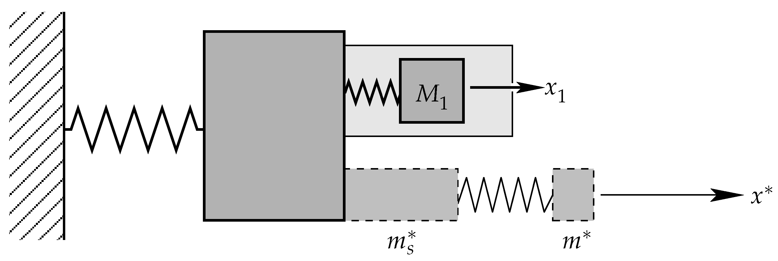
5.9. TMD with Inerter

A mechanical device called the inerter has been proposed [32], which is attached to two points and uses a flywheel to resist the relative motion of the two points, in effect simulating a large kinetic mass, which can greatly exceed the mass of the inerter itself. One proposed application of the inerter for vibration damping is given in [33] and shown in Figure 10. The inerter, whose mass is $M_{\mathrm{in}.}^{\prime }$, adds a kinetic energy $\frac{1}{2}{M}_{\mathrm{in}.}{\dot{x}}_1^2$, where $M_{\mathrm{in}.}\gg M_{\mathrm{in}.}^{\prime }$. Comparing to the discussion of added mass in Section 3 (see Equations (3)–(5)), we note that the inerter simply increases the kinetic energy mass $M_K$ associated with the TMD. The effective TMD mass is then $m_{}^{*}=\frac{M_1^2}{M_1^{}+M_{\mathrm{in}.}}$. This explains Figure 2 in [33].

The inerter acts to effectively bind part of the combined mass of all the damper components $M_T^{}$ to the structure, with $m_s^{*}=M_T-m^{*}$. On the other hand, the motion amplitude of the TMD with inerter is smaller than that of the equivalent simple TMD, with $x^{*}=(1+\frac{M_{\mathrm{in}.}}{M_1})x_1$. Therefore, adding an inerter to a TMD in the proposed configuration is equivalent to replacing the TMD with a smaller TMD.

6. Summary and Conclusions

The presence of added mass, i.e., mass moving in other directions than that of the structural motion, reduces the effective TMD mass to a lower value than might be expected from a naive interpretation. This is due to the fact that added mass impedes the movement within the damper, effectively reducing the damper motion amplitude. This leads to a reduced effective mass ratio, which in turn influences the optimal damper parameters. A failure to correctly account for the role of added mass in the effective TMD mass leads to an overestimated mass ratio and to sub-optimal damper parameters.

We have seen above how general TMDs can be treated in a simple way by the introduction of an equivalent simple TMD. The theory was developed in Section 3 and Section 4. When analyzing a given general TMD, one simply has to compute three masses: The total mass, the inertial mass and the kinetic energy mass by Equations (3)–(5). Then, one applies Equations (11)–(13) and (14)–(15) in order to obtain the equivalent simple TMD parameters and the effective mass ratio. This straightforward method makes analysis and optimization of general TMDs easy.

The theory has been applied to a number of systems in Section 5. TMDs of certain types, including TLDs and TLCDs, have been shown to operate with significant added mass, leading to a smaller equivalent simple TMD mass than might be expected.

The developed framework provides a practical tool for analyzing and tuning general TMDs with added mass. The method is versatile and can be used for purely mechanical systems, as well as systems with coupled motion of fluid and solid components. In fact, any linear one degree-of-freedom system can be analyzed. The framework enables using well-known and proven TMD tuning methods on a very broad range of TMDs.

The authors hope that this work may alleviate some of the confusion surrounding TMDs with added mass and provide a useful practical tool for both researchers and engineers.