
Identifying Influential Spatial Drivers of Forest Fires through Geographically and Temporally Weighted Regression Coupled with a Continuous Invasive Weed Optimization Algorithm


Abstract
:1. Introduction
2. Materials and Methods
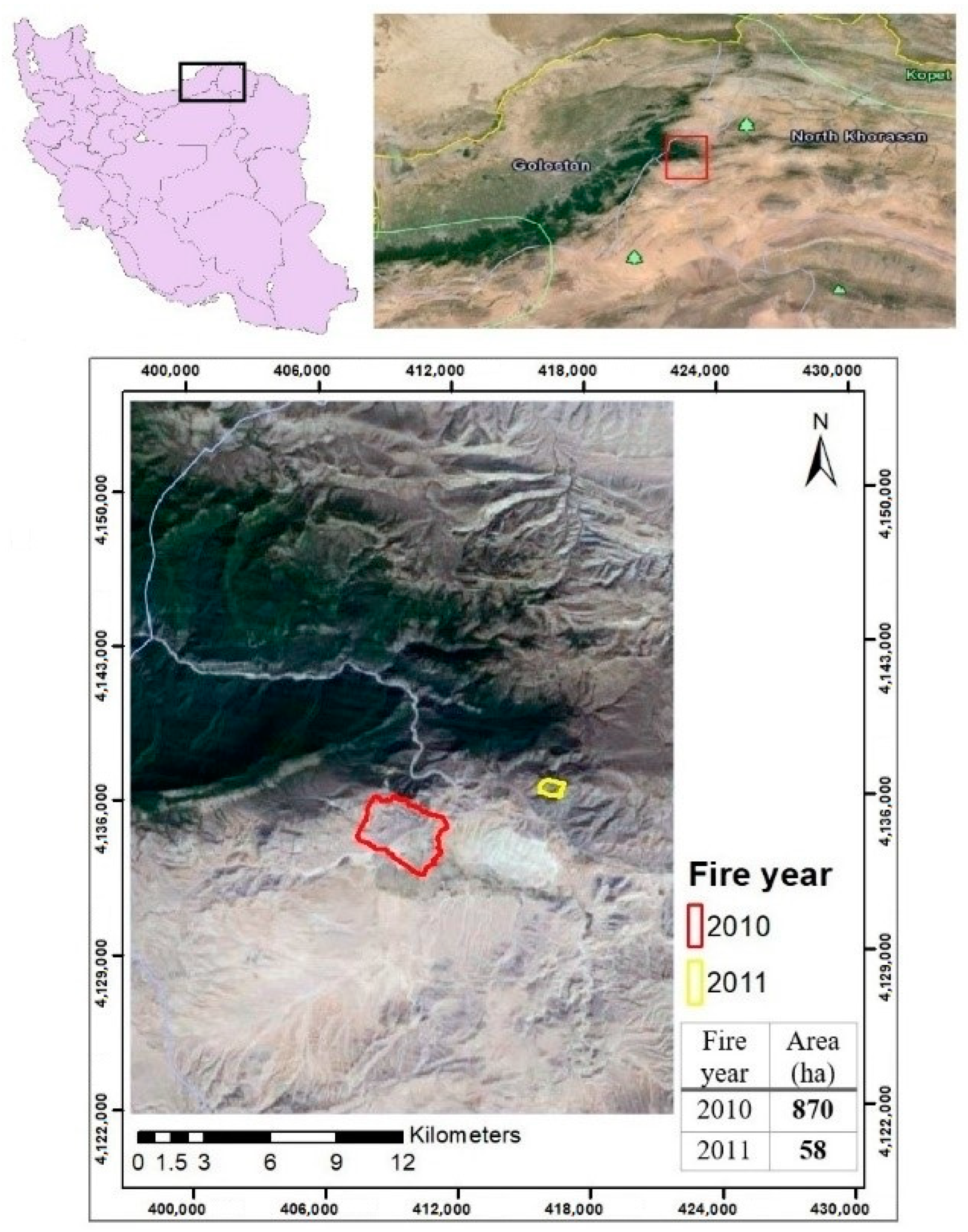
2.1. Study Area
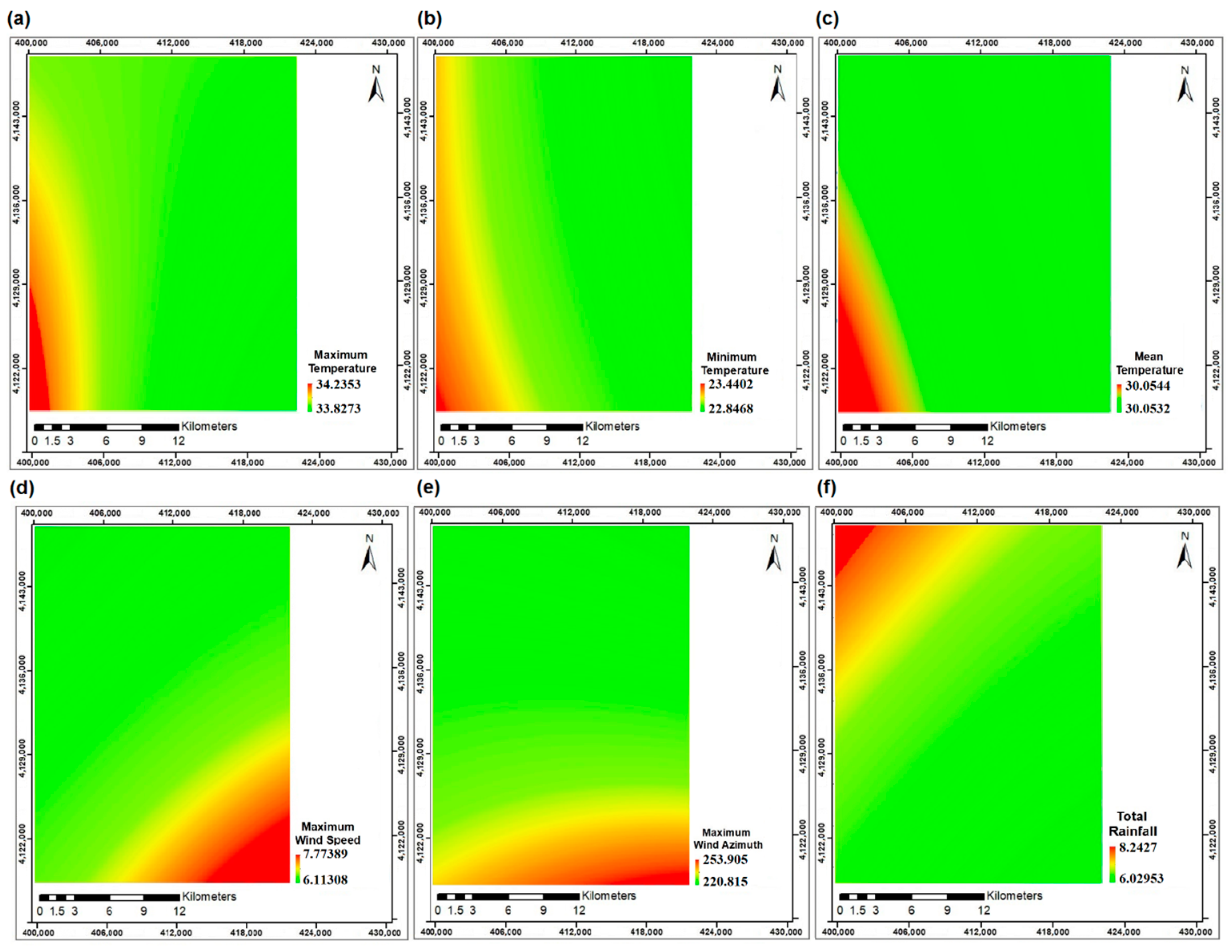
2.2. Datasets
2.3. Geographically Weighted Regression (GWR)
2.4. Geographically and Temporally Weighted Regression (GTWR)
| Algorithm 1 The proposed GTWR pseudo-code for this study |
| Select the optimal bandwidth parameter using Cross Validation. Calculate the spatiotemporal distance among all pairs of the points. Calculate the geographic weights using Tricube kernel. Calculate the coefficients of regression Calculate the Coefficient of Determination. return the coefficients of regression; the Coefficient of Determination; the residuals; the estimated values of observations; the used kernel type; the optimal bandwidth; the t-statistics matrix; the iteration of Cross Validation; the estimated standard deviation of residuals; the input parameters of the GTWR method. |
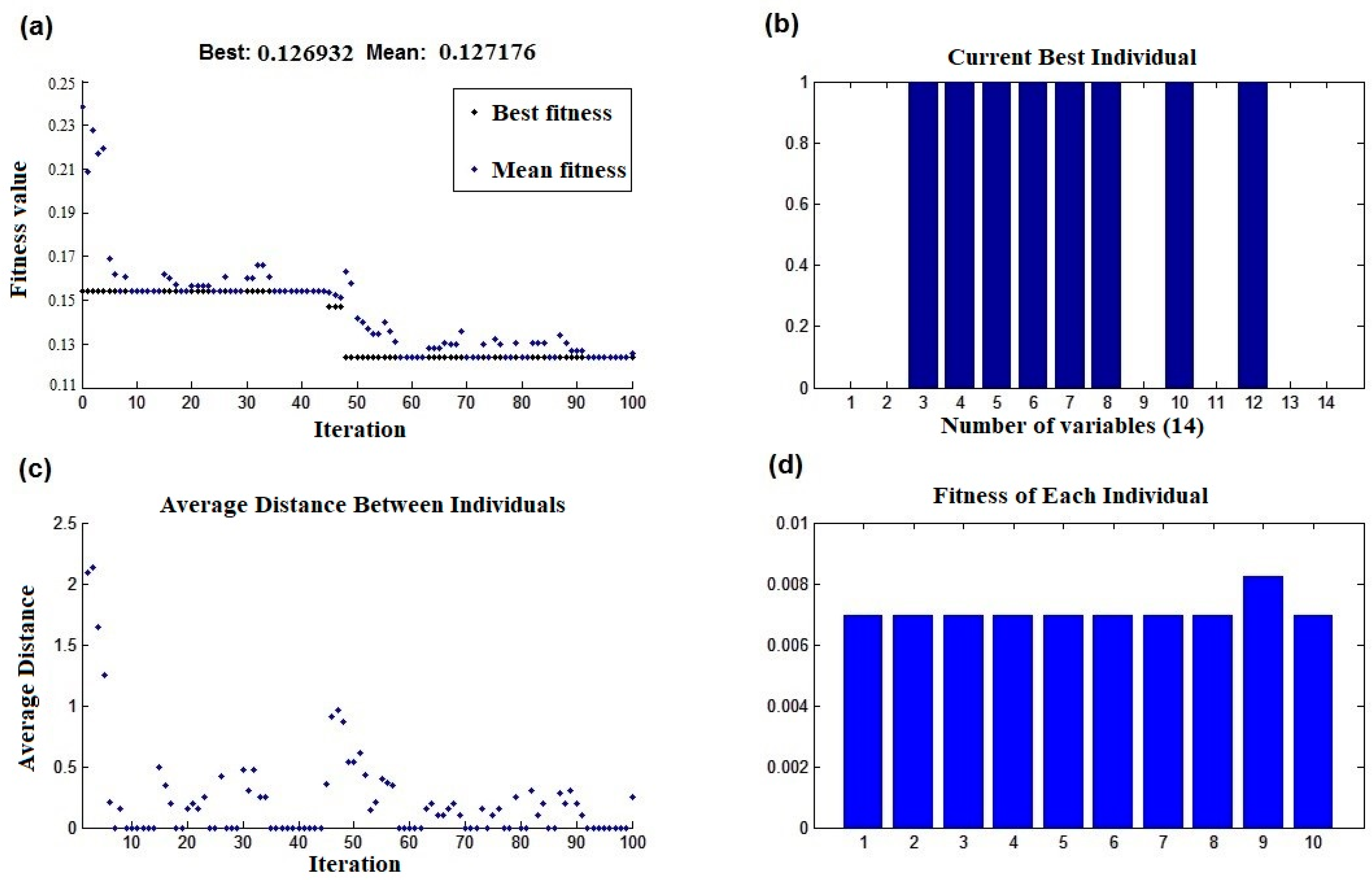
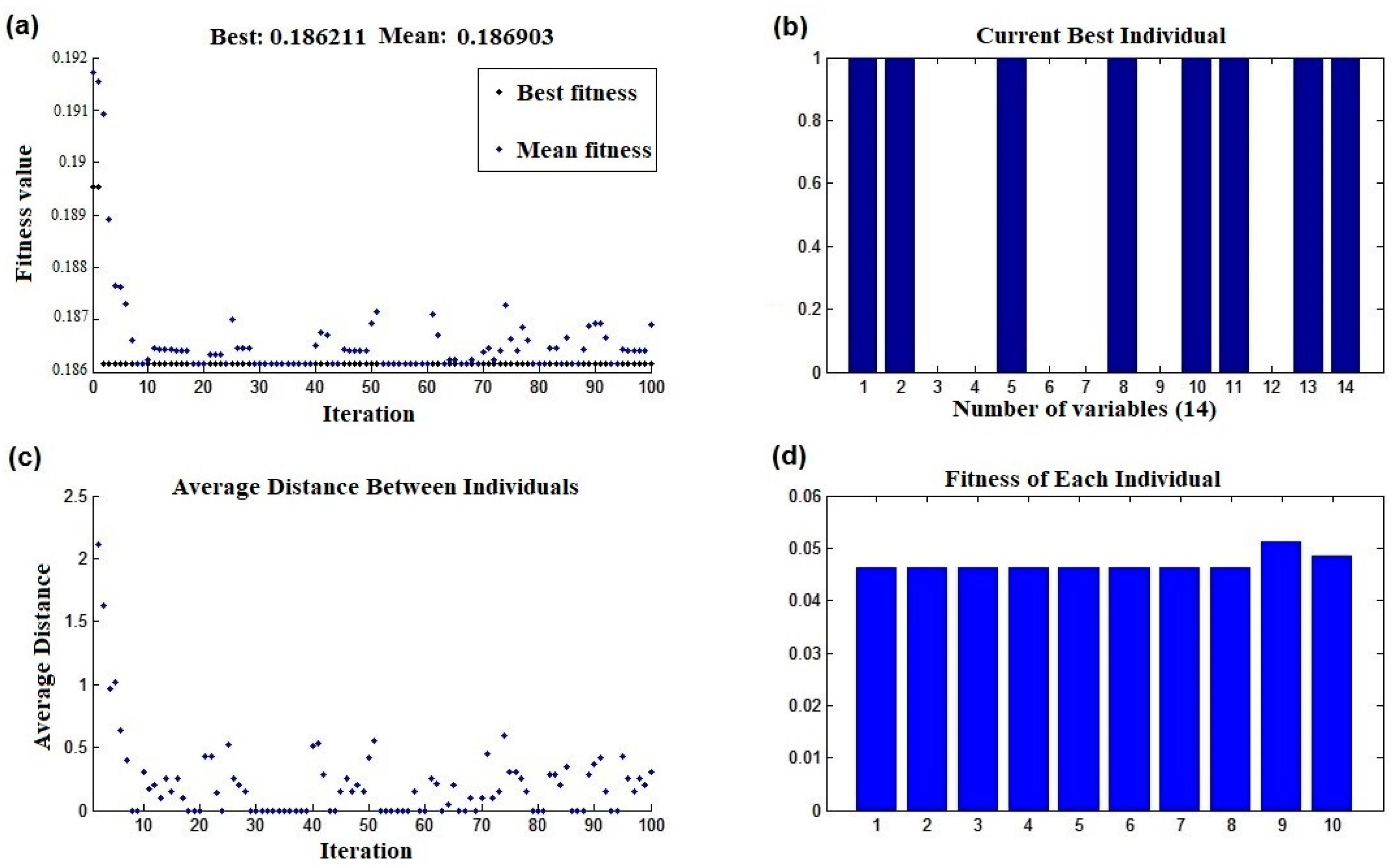
2.5. Selection of the Optimum Spatial Factors
| Algorithm 2 The pseudo-code of the proposed algorithm for selecting spatial factors with the most effects on forest fires |
| Create a d-dimenonal weed position vector P times (P < Pmax) with a uniformly random values αi ∈ (0,1) for i = 1 to d, where d is the number of spatial factors do for each iteration (it = l to itmax) do Calculate cit based on Equation (21); end for for each weed (k = l to P) do Calculate the fiuess, i.e., the l-R2, based on Equation (10) for αi where αi> σth; end for while it <= itmax do for each weed k do Calculate the number of seeds [Equation (20)]; Randomly disperse the generated seeds over the search-space Equations (21)–(23); Add the generated seeds at the end of the population; Calculate the fitess of the generated seeds, i.e., the l-R2, based on Equation (10) for αi where αi> σth; end for if P > Pmax then Sort the population in deseending order of their l-R²; Eliminate population of weeds with higher l-R² till P = Pmax; end if end while return the selected spatial factors (αi where αi > σth) for the weed with the best fitness; |
3. Results
4. Discussion
5. Conclusions
Author Contributions
Funding
Institutional Review Board Statement
Informed Consent Statement
Data Availability Statement
Conflicts of Interest
References
- Eskandari, S.; Miesel, J.R.; Pourghasemi, H.R. The temporal and spatial relationships between climatic parameters and fire occurrence in northeastern Iran. Ecol. Indic. 2022, 118, 106720. [Google Scholar] [CrossRef]
- Pang, Y.; Li, Y.; Feng, Z.; Feng, Z.; Zhao, Z.; Chen, S.; Zhang, H. Forest fire occurrence prediction in China based on machine learning methods. Remote Sens. 2022, 14, 5546. [Google Scholar] [CrossRef]
- Ma, W.; Feng, Z.; Cheng, Z.; Chen, S.; Wang, F. Identifying Forest Fire Driving Factors and Related Impacts in China Using Random Forest Algorithm. Forests 2020, 11, 507. [Google Scholar] [CrossRef]
- McKenzie, D.C.; Shankar, U.; Keane, R.E.; Stavros, E.N.; Heilman, W.E.; Fox, D.G.; Riebau, A.C. Smoke Consequences of New Wildfire Regimes Driven by Climate Change. Earth’s Future 2014, 2, 35–59. [Google Scholar] [CrossRef]
- Saha, S.; Bera, B.; Shit, P.K.; Bhattacharjee, S.; Sengupta, N. Prediction of Forest Fire Susceptibility Applying Machine and Deep Learning Algorithms for Conservation Priorities of Forest Resources. Remote Sens. Appl. Soc. Environ. 2023, 29, 100917. [Google Scholar] [CrossRef]
- Kolanek, A.; Szymanowski, M.; Raczyk, A. Human Activity Affects Forest Fires: The Impact of Anthropogenic Factors on the Density of Forest Fires in Poland. Forests 2021, 12, 728. [Google Scholar]
- Ghorbanzadeh, O.; Blaschke, T.; Gholamnia, K.; Aryal, J. Forest Fire Susceptibility and Risk Mapping Using Social/infrastructural Vulnerability and Environmental Variables. Fire 2019, 2, 50. [Google Scholar] [CrossRef]
- Su, Z.; Tigabu, M.; Cao, Q.; Wang, G.; Hu, H.; Guo, F. Comparative Analysis of Spatial Variation in Forest Fire Drivers between Boreal and Subtropical Ecosystems in China. For. Ecol. Manag. 2019, 454, 117669. [Google Scholar] [CrossRef]
- Massetti, A.; Rudiger, C.; Yebra, M.; Yebra, M.; Hilton, J.E.; Hilton, J.E. The Vegetation Structure Perpendicular Index (VSPI): A Forest Condition Index for Wildfire Predictions. Remote Sens. Environ. 2019, 224, 167–181. [Google Scholar]
- Dickson, B.G.; Prather, J.W.; Xu, Y.; Hampton, H.M.; Aumack, E.N.; Sisk, T.D. Mapping the Probability of Large Fire Occurrence in Northern Arizona, USA. Landsc. Ecol. 2006, 21, 747–761. [Google Scholar]
- Arif, M.; Alghamdi, K.K.; Sahel, S.A.; Alosaimi, S.O.; Alsahaft, M.E.; Alharthi, M.A.; Arif, M. Role of Machine Learning Algorithms in Forest Fire Management: A Literature Review. J. Robot. Autom. 2021, 5, 212–226. [Google Scholar]
- Mukunga, T.; Forkel, M.; Forrest, M.; Zotta, R.M.; Pande, N.; Schlaffer, S.; Dorigo, W. Effect of Socioeconomic Variables in Predicting Global Fire Ignition Occurrence. Fire 2023, 6, 197. [Google Scholar] [CrossRef]
- Martínez-Fernández, J.; Chuvieco, E.; Koutsias, N. Modelling Long-term Fire Occurrence Factors in Spain by Accounting for Local Variations with Geographically Weighted Regression. Nat. Hazards Earth Syst. Sci. 2013, 13, 311–327. [Google Scholar] [CrossRef]
- Mercer, D.E.; Prestemon, J.P. Comparing Production Function Models for Wildfire Risk Analysis in the Wildland–urban Interface. For. Policy Econ. 2005, 7, 782–795. [Google Scholar] [CrossRef]
- Moritz, M.A.; Keeley, J.E.; Johnson, E.A.; Schaffner, A. Testing a Basic Assumption of Shrubland Fire Management: How Important Is Fuel Age? Front. Ecol. Environ. 2004, 2, 67–72. [Google Scholar]
- Roman-Cuesta, R.M.; Martínez-Vilalta, J. Effectiveness of Protected Areas in Mitigating Fire within Their Boundaries: Case Study of Chiapas, Mexico. Conserv. Biol. 2006, 20, 1074–1086. [Google Scholar]
- Syphard, A.D.; Radeloff, V.C.; Keuler, N.S.; Taylor, R.S.; Hawbaker, T.J.; Stewart, S.I.; Clayton, M.K. Predicting Spatial Patterns of Fire on a Southern California Landscape. Int. J. Wildland Fire 2008, 17, 602–613. [Google Scholar]
- Murthy, K.K.; Sinha, S.K.; Kaul, R.; Vaidyanathan, S. A fine-scale state-space model to understand drivers of forest fires in the Himalayan foothills. For. Ecol. Manag. 2019, 432, 902–911. [Google Scholar] [CrossRef]
- Romero-Calcerrada, R.; Novillo, C.J.; Millington, J.D.A.; Gomez-Jimenez, I. GIS Analysis of Spatial Patterns of Human-caused Wildfire Ignition Risk in the SW of Madrid (central Spain). Landsc. Ecol. 2008, 23, 341–354. [Google Scholar] [CrossRef]
- Erten, E.; Kurgun, V.; Musaoglu, N. Forest fire risk zone mapping from satellite imagery and GIS: A case study. In Proceedings of the XXth Congress of the International Society for Photogrammetry and Remote Sensing, Istanbul, Turkey, 12–23 July 2004. [Google Scholar]
- Bufacchi, P.; Krieger, G.C.; Mell, W.; Alvarado, E.; Santos, J.C.; de Carvalho, J.A. Numerical Simulation of Surface Forest Fire in Brazilian Amazon. Fire Saf. J. 2016, 79, 44–56. [Google Scholar]
- Zhang, Y.; Lim, S.; Sharples, J.J. Modelling Spatial Patterns of Wildfire Occurrence in South-eastern Australia. Geomat. Nat. Hazards Risk 2016, 7, 1800–1815. [Google Scholar]
- Joseph, M.B.; Rossi, M.W.; Mietkiewicz, N.; Mahood, A.L.; Cattau, M.E.; St. Denis, L.A.; Nagy, R.C.; Iglesias, V.; Abatzoglou, J.T.; Balch, J.K. Spatiotemporal Prediction of Wildfire Size Extremes with Bayesian Finite Sample Maxima. Ecol. Appl. 2019, 29, e01898. [Google Scholar] [PubMed]
- Jaafari, A.; Pourghasemi, H.R. Factors influencing regional-scale wildfire probability in Iran: An application of random forest and support vector machine. In Spatial Modeling in GIS and R for Earth and Environmental Sciences; Elsevier: Amsterdam, The Netherlands, 2019; pp. 607–619. [Google Scholar]
- Milanović, S.; Kaczmarowski, J.; Ciesielski, M.; Trailović, Z.; Mielcarek, M.; Szczygieł, R.; Milanović, S.D. Modeling and mapping of forest fire occurrence in the Lower Silesian Voivodeship of Poland based on Machine Learning methods. Forests 2023, 14, 46. [Google Scholar]
- Ávila-Flores, D.Y.; Pompa-García, M.; Antonio-Nemiga, X.; Rodríguez-Trejo, D.A.; Vargas-Perez, E.; Santillan-Perez, J. Driving Factors for Forest Fire Occurrence in Durango State of Mexico: A Geospatial Perspective. Chin. Geogr. Sci. 2010, 20, 491–497. [Google Scholar] [CrossRef]
- Koutsias, N.; Martínez-Fernández, J.; Allgöwer, B. Do Factors Causing Wildfires Vary in Space? Evidence from Geographically Weighted Regression. GIScience Remote Sens. 2010, 47, 221–240. [Google Scholar] [CrossRef]
- Ávila-Flores, D.Y.; Pompa-Garcia, M.; Vargas-Perez, E. Spatial analysis of forest fire occurrence in the state of Durango. Rev. Chapingo Ser. Cienc. For. Ambiente 2010, 16, 253–260. [Google Scholar]
- Sá, A.C.L.; Pereira, J.M.C.; Charlton, M.; Mota, B.; Barbosa, P.; Fotheringham, A.S. The Pyrogeography of Sub-saharan Africa: A Study of the Spatial Non-stationarity of Fire–environment Relationships Using GWR. J. Geogr. Syst. 2011, 13, 227–248. [Google Scholar]
- Akhani, H. Plant Biodiversity of Golestan National Park, Iran; OÖ Landesmuseum, Biologiezentrum: Linz, Austria, 1998; Volume 53. [Google Scholar]
- Jahdi, R.; Bacciu, V.; Salis, M.; Del Giudice, L.; Cerdà, A. Surface Wildfire Regime and Simulation-Based Wildfire Exposure in the Golestan National Park, NE Iran. Fire 2023, 6, 244. [Google Scholar]
- Akhani, H. Studies on the flora and vegetation of the Golestan National Park, NE Iran. III. Three new species, one new subspecies and fifteen new records for Iran. Edinb. J. Bot. 1999, 56, 1–31. [Google Scholar] [CrossRef]
- Ziary, Y.; Safari, H. To Compare Two Interpolation Methods: IDW, Kriging for Providing Properties (Area) Surface Interpolation Map Land Price. District 5, Municipality of Tehran area 1. In Proceedings of the FIG Working Week, Hong Kong, China, 13 May 2007; Volume 13. [Google Scholar]
- Shekhar, S.; Xiong, H. Encyclopedia of GIS; Springer Publishing Company, Incorporated: Berlin/Heidelberg, Germany, 2007. [Google Scholar]
- Brunsdon, C.; Fotheringham, S.; Charlton, M. Geographically Weighted Regression-Modelling Spatial Non-Stationarity. Statistician 1998, 47, 431–443. [Google Scholar]
- McMillen, D.P.; McDonald, J.F. Locally Weighted Maximum Likelihood Estimation: Monte Carlo Evidence and an Application. In Advances in Spatial Econometrics: Methodology, Tools and Applications; Springer: Berlin/Heidelberg, Germany, 2004. [Google Scholar]
- Charlton, M.; Fotheringham, S.; Brunsdon, C. Geographically Weighted Regression; White Paper; National Centre for Geocomputation, National University of Ireland Maynooth: Kildare, Ireland, 2009. [Google Scholar]
- Huang, B.; Wu, B.; Barry, M. Geographically and Temporally Weighted Regression for Modeling Spatio-temporal Variation in House Prices. Int. J. Geogr. Inf. Sci. 2010, 24, 383–401. [Google Scholar] [CrossRef]


| Symbol | Quantity | Value |
|---|---|---|
| P | Number of initial populations | 5 |
| Pmax | Maximum number of plant populations | 20 |
| itmax | Maximum number of iterations | 100 |
| Nmax | Maximum number of seeds | 3 |
| Nmin | Minimum number of seeds | 0 |
| ci | Initial standard deviation value from a parent weed | 0.7 |
| cf | Final standard deviation value from a parent weed | 0.3 |
| m | Non-linear modulation indexes | 3 |
| Threshold for selecting factors from a weed | 0.5 |
| Factor | Standard Deviation with Tricube Kernel | Standard Deviation with Gaussian Kernel |
|---|---|---|
| Constant coefficient | 5.057858 | 1.733206 |
| Distance from rivers (m) | - | 0.000086 |
| Distance from roads (m) | - | 0.000114 |
| Distance from residential zones (m) | 0.005284 | - |
| Soil type | 2.895782 | - |
| Land use | 6.814788 | 0.056198 |
| Elevation (m) | 0.011047 | - |
| Slope | 0.024342 | - |
| Aspect | 0.007365 | 0.000169 |
| Maximum temperature (°C) | - | - |
| Minimum temperature (°C) | 8.9964 | 6.28476 |
| Mean temperature (°C) | - | 5.10398 |
| Maximum wind azimuth | 1.720777 | - |
| Maximum wind speed (m/s) | - | 0.746954 |
| Total rainfall (mm) | - | 8.72719 |
| Factor | Standard Deviation with Tricube Kernel | Standard Deviation with Gaussian Kernel |
|---|---|---|
| Constant coefficient | 0.185946 | 0.091358 |
| Distance from rivers (m) | - | - |
| Distance from roads (m) | - | - |
| Distance from residential zones (m) | 0.00117 | 0.000557 |
| Soil type | 2.45784 | - |
| Land use | - | 0.027503 |
| Elevation (m) | 0.004852 | 0.000995 |
| Slope | 0.002745 | - |
| Aspect | 0.000454 | - |
| Maximum temperature (°C) | - | 1.663826 |
| Minimum temperature (°C) | 3.87414 | 4.244687 |
| Mean temperature (°C) | - | 2.741073 |
| Maximum wind azimuth | - | 0.52631 |
| Maximum wind speed (m/s) | 5.57909 | - |
| Total rainfall (mm) | - | - |
| Factor | Standard Deviation with Tricube Kernel | Standard Deviation with Gaussian Kernel |
|---|---|---|
| Constant coefficient | 0.0795 | 14.23006 |
| Distance from rivers (m) | 0.0004 | 0.001235 |
| Distance from roads (m) | - | 0.000958 |
| Distance from residential zones (m) | - | 0.000427 |
| Soil type | 0.2173 | - |
| Land use | - | 5.909925 |
| Elevation (m) | - | 0.001698 |
| Slope | - | 0.053385 |
| Aspect | - | 0.000395 |
| Maximum temperature (°C) | 0.6545 | 3.305766 |
| Minimum temperature (°C) | - | 2.640458 |
| Mean temperature (°C) | - | 5.265534 |
| Maximum wind azimuth | 0.1471 | 0.063351 |
| Maximum wind speed (m/s) | 0.9536 | 3.130694 |
| Total rainfall (mm) | 0.1256 | 0.116119 |
| Kernel | RMSE | NRMSE |
|---|---|---|
| Tricube | 0.020937 | 0.048433 |
| Gaussian | 0.095936 | 0.229325 |
| Kernel | RMSE | NRMSE |
|---|---|---|
| Tricube | 0.020062 | 0.042741 |
| Gaussian | 0.039408 | 0.099447 |
| Kernel | RMSE | NRMSE |
|---|---|---|
| Tricube | 0.014545 | 0.039068 |
| Gaussian | 0.060122 | 0.165425 |
| Predicted Fire Cells | Predicted Non-Fire Cells | |
| Observed fire cells | 9322 | 347 |
| Observed non-fire cells | 3951 | 729,536 |
| Predicted Fire Cells | Predicted Non-Fire Cells | |
| Observed fire cells | 647 | 0 |
| Observed non-fire cells | 2787 | 739,722 |
| 17 November 2010 | 15 July 2011 | |
| Error Rate (%) | 0.58 | 0.38 |
| Accuracy (%) | 99.42 | 99.62 |
| Sensitivity (%) | 96.41 | 100 |
| Specificity (%) | 99.62 | 99.46 |
Disclaimer/Publisher’s Note: The statements, opinions and data contained in all publications are solely those of the individual author(s) and contributor(s) and not of MDPI and/or the editor(s). MDPI and/or the editor(s) disclaim responsibility for any injury to people or property resulting from any ideas, methods, instructions or products referred to in the content. |
© 2024 by the authors. Licensee MDPI, Basel, Switzerland. This article is an open access article distributed under the terms and conditions of the Creative Commons Attribution (CC BY) license (https://creativecommons.org/licenses/by/4.0/).
Share and Cite
Pahlavani, P.; Raei, A.; Bigdeli, B.; Ghorbanzadeh, O. Identifying Influential Spatial Drivers of Forest Fires through Geographically and Temporally Weighted Regression Coupled with a Continuous Invasive Weed Optimization Algorithm. Fire 2024, 7, 33. https://doi.org/10.3390/fire7010033
Pahlavani P, Raei A, Bigdeli B, Ghorbanzadeh O. Identifying Influential Spatial Drivers of Forest Fires through Geographically and Temporally Weighted Regression Coupled with a Continuous Invasive Weed Optimization Algorithm. Fire. 2024; 7(1):33. https://doi.org/10.3390/fire7010033
Chicago/Turabian StylePahlavani, Parham, Amin Raei, Behnaz Bigdeli, and Omid Ghorbanzadeh. 2024. "Identifying Influential Spatial Drivers of Forest Fires through Geographically and Temporally Weighted Regression Coupled with a Continuous Invasive Weed Optimization Algorithm" Fire 7, no. 1: 33. https://doi.org/10.3390/fire7010033