


Forest Fire Driving Factors and Fire Risk Zoning Based on an Optimal Parameter Logistic Regression Model: A Case Study of the Liangshan Yi Autonomous Prefecture, China
 , ,
, ,
Abstract
:1. Introduction
2. Materials and Methods
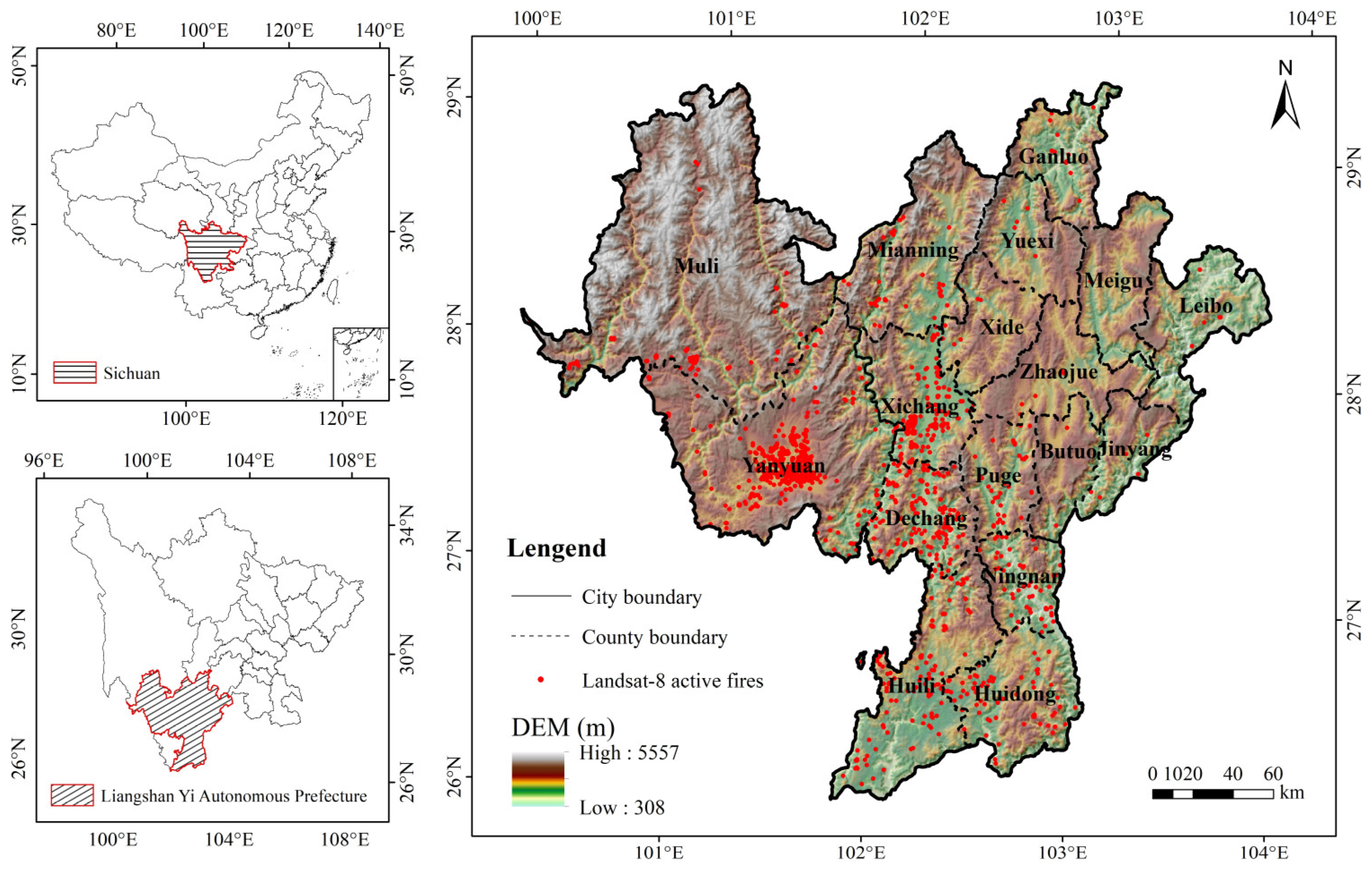
2.1. Study Area
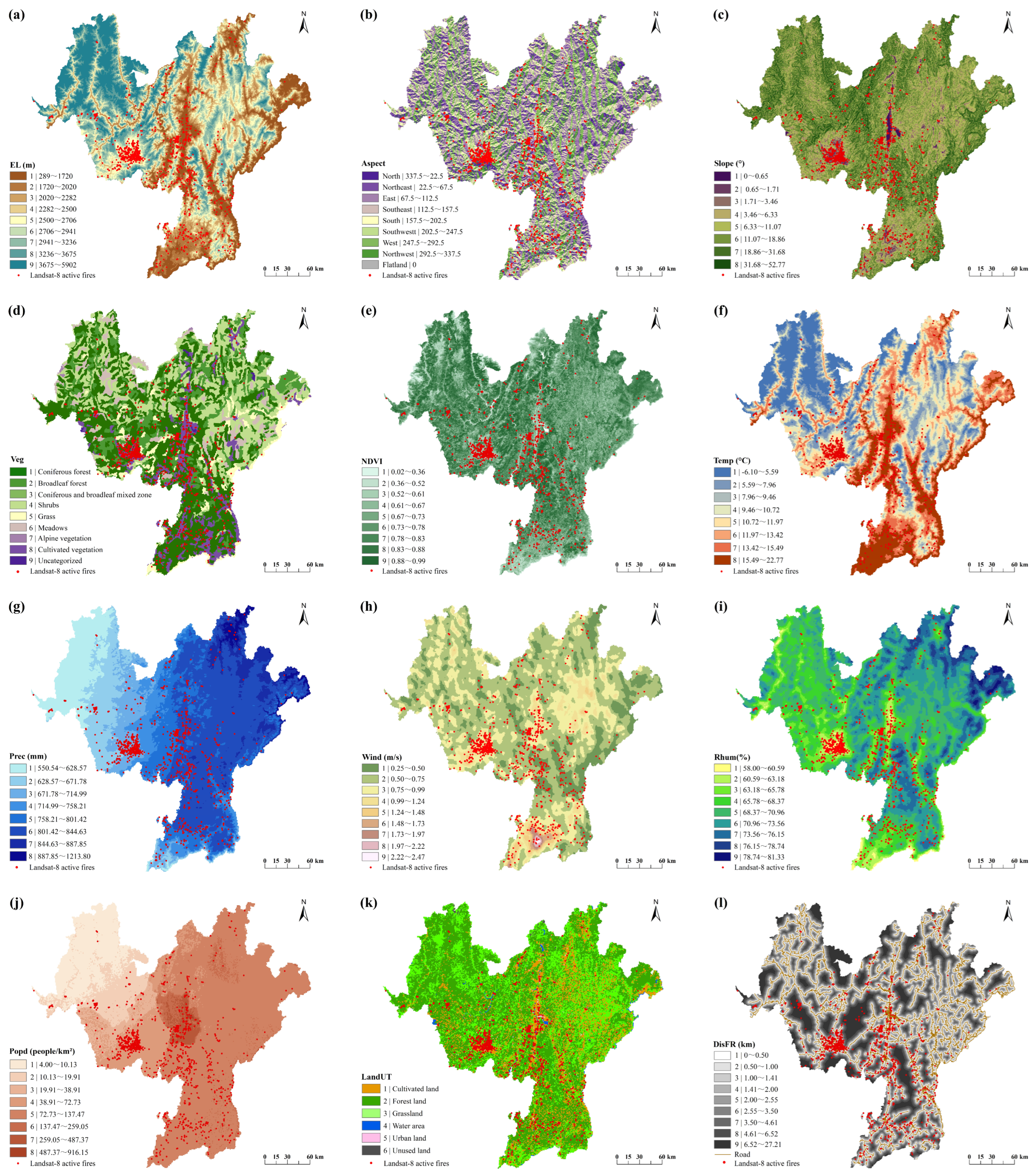
2.2. Data Sources
2.3. Optimal Parameter-Based Geographical Detector Model
2.4. Logistic Forest Fire Regression Prediction Model
2.5. Spearman Rank Correlation Coefficient
2.6. Multicollinearity Analysis
2.7. Receiver Operator Characteristic (ROC) Curve Analysis
3. Results
3.1. Spatial Unit and Discretization of Optimal Parameters
3.2. Results of the Spearman Rank Correlation Coefficient
3.3. Results of the Driving Factor Multicollinearity Diagnosis
3.4. Construction and Evaluation of the OPLR Forest Fire Prediction Model
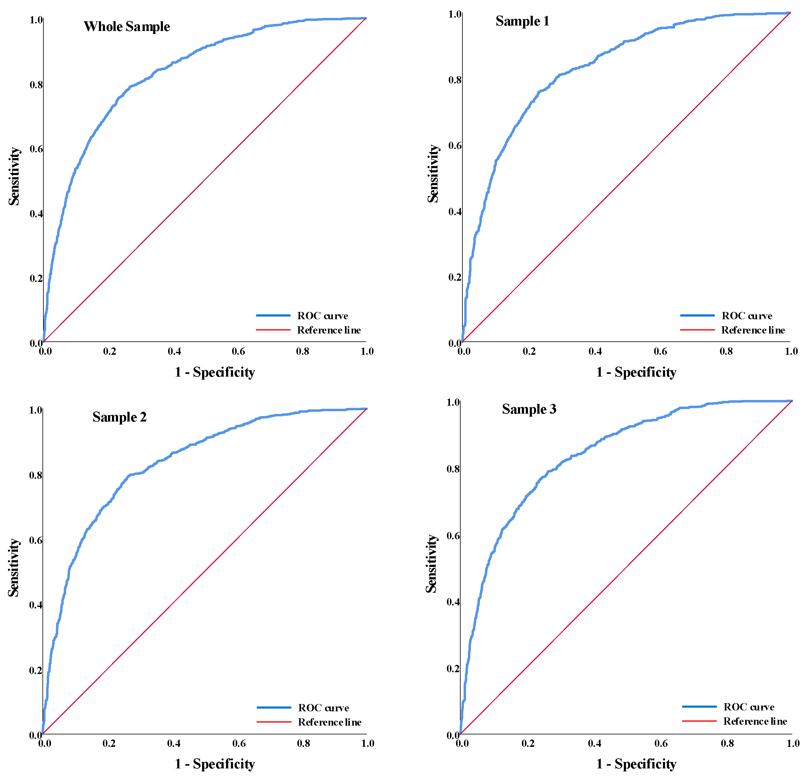
3.5. ROC Curve Analysis
3.6. Classification of Forest Fire Probability Risk Level
4. Discussion
4.1. Effects of Meteorological Factors on Forest Fires
4.2. Effects of Topographic Factors and Vegetation Factors on Forest Fires
4.3. Effects of Human Factors on Forest Fires
4.4. Limitations and Future Developments
5. Conclusions
Author Contributions
Funding
Data Availability Statement
Acknowledgments
Conflicts of Interest
References
- Hong, H.; Tsangaratos, P.; Ilia, I.; Liu, J.; Zhu, A.-X.; Xu, C. Applying Genetic Algorithms to Set the Optimal Combination of Forest Fire Related Variables and Model Forest Fire Susceptibility Based on Data Mining Models. The case of Dayu County, China. Sci. Total Environ. 2018, 630, 1044–1056. [Google Scholar] [CrossRef] [PubMed]
- Sowmya, S.; Somashekar, R. Application of Remote Sensing and Geographical Information System in Mapping Forest Fire Risk Zone at Bhadra Wildlife Sanctuary, India. J. Environ. Sci. 2010, 31, 969–974. [Google Scholar]
- Li, J.Y.; Chen, C. Modeling the Dynamics of Disaster Evolution Along Causality Networks with Cycle Chains. Phys. A Stat. Mech. Its Appl. 2014, 401, 251–264. [Google Scholar] [CrossRef]
- Zhang, J.-H.; Li, J.; Liu, Z. Multiple-Resource and Multiple-depot Emergency Response Problem Considering Secondary Disasters. Expert Syst. Appl. 2012, 39, 11066–11071. [Google Scholar] [CrossRef]
- Rengers, F.K.; McGuire, L.A.; Oakley, N.S.; Kean, J.W.; Staley, D.M.; Tang, H. Landslides After Wildfire: Initiation, Magnitude, and Mobility. Landslides 2020, 17, 2631–2641. [Google Scholar] [CrossRef]
- Dong, S.Y.; Jiang, Y.S.; Yu, X. Analyses of the Impacts of Climate Change and Forest Fire on Cold Region Slopes Stability by Random Finite Element Method. Landslides 2021, 18, 2531–2545. [Google Scholar] [CrossRef]
- Pacheco, A.P.; Claro, J.; Fernandes, P.M.; de Neufville, R.; Oliveira, T.M.; Borges, J.G.; Rodrigues, J.C. Cohesive Fire Management within an Uncertain Environment: A Review of Risk Handling and Decision Support Systems. For. Ecol. Manag. 2015, 347, 1–17. [Google Scholar] [CrossRef]
- Akay, A.E.; Wing, M.G.; Zengin, M.; Kose, O. Determination of Fire-access Zones along Road Networks in Fire-Sensitive Forests. J. For. Res. 2017, 28, 557–564. [Google Scholar] [CrossRef]
- Enoh, M.A.; Okek, U.C.; Narinua, N.Y. Identification and Modelling of Forest Fire Severity and Risk Zones in the Cross-Niger Transition Forest with Remotely Sensed Satellite Data. Egypt. J. Remote Sens. Space Sci. 2021, 24, 879–887. [Google Scholar] [CrossRef]
- Pang, Y.Q.; Li, Y.D.; Feng, Z.K.; Feng, Z.M.; Zhao, Z.Y.; Chen, S.L.; Zhang, H.Y. Forest Fire Occurrence Prediction in China Based on Machine Learning Methods. Remote Sens. 2022, 14, 5546. [Google Scholar] [CrossRef]
- Guo, F.T.; Su, Z.W.; Wang, G.Y.; Sun, L.; Tigabu, M.; Yang, X.J.; Hu, H.Q. Understanding Fire Drivers and Relative Impacts in Different Chinese Forest Ecosystems. Sci. Total Environ. 2017, 605, 411–425. [Google Scholar] [CrossRef] [PubMed]
- Pan, J.H.; Wang, W.G.; Li, J.F. Building Probabilistic Models of Fire Occurrence and Fire Risk Zoning Using Logistic Regression in Shanxi Province, China. Nat. Hazards 2016, 81, 1879–1899. [Google Scholar] [CrossRef]
- Tian, Y.P.; Wu, Z.C.; Li, M.Z.; Wang, B.; Zhang, X.D. Forest Fire Spread Monitoring and Vegetation Dynamics Detection Based on Multi-Source Remote Sensing Images. Remote Sens. 2022, 14, 4431. [Google Scholar] [CrossRef]
- Ciesielski, M.; Balazy, R.; Borkowski, B.; Szczesny, W.; Zasada, M.; Kaczmarowski, J.; Kwiatkowski, M.; Szczygiel, R.; Milanovic, S. Contribution of Anthropogenic, Vegetation, and Topographic Features to Forest Fire Occurrence in Poland. Iforest Biogeosci. For. 2022, 15, 307–314. [Google Scholar] [CrossRef]
- Marchal, J.; Cumming, S.G.; McIntire, E.J.B. Turning Down the Heat: Vegetation Feedbacks Limit Fire Regime Responses to Global Warming. Ecosystems 2020, 23, 204–216. [Google Scholar] [CrossRef]
- Girardin, M.P.; Ali, A.A.; Carcaillet, C.; Gauthier, S.; Hely, C.; Le Goff, H.; Terrier, A.; Bergeron, Y. Fire in Managed Forests of Eastern Canada: Risks and Options. For. Ecol. Manag. 2013, 294, 238–249. [Google Scholar] [CrossRef]
- Shmuel, A.; Ziv, Y.; Heifetz, E. Machine-Learning-Based Evaluation of the Time-Lagged Effect of Meteorological Factors On 10-Hour Dead Fuel Moisture Content. For. Ecol. Manag. 2022, 505, 119897. [Google Scholar] [CrossRef]
- Ng, J.; North, M.P.; Arditti, A.J.; Cooper, M.R.; Lutz, J.A. Topographic Variation in Tree Group and Gap Structure in Sierra Nevada Mixed-Conifer Forests with Active Fire Regimes. For. Ecol. Manag. 2020, 472, 118220. [Google Scholar] [CrossRef]
- Loudermilk, E.L.; O’Brien, J.J.; Goodrick, S.L.; Linn, R.R.; Skowronski, N.S.; Hiers, J.K. Vegetation’s Influence on Fire Behavior Goes Beyond Just Being Fuel. Fire Ecol. 2022, 18, 1–10. [Google Scholar] [CrossRef]
- Liang, S.; Hurteau, M.D. Novel Climate-Fire-Vegetation Interactions and Their Influence on Forest Ecosystems in the Western USA. Funct. Ecol. 2023, 37, 2126–2142. [Google Scholar] [CrossRef]
- Ying, L.X.; Han, J.; Du, Y.S.; Shen, Z.H. Forest Fire Characteristics in China: Spatial Patterns and Determinants with Thresholds. For. Ecol. Manag. 2018, 424, 345–354. [Google Scholar] [CrossRef]
- Ganteaume, A.; Camia, A.; Jappiot, M.; San-Miguel-Ayanz, J.; Long-Fournel, M.; Lampin, C. A Review of the Main Driving Factors of Forest Fire Ignition Over Europe. Environ. Manag. 2013, 51, 651–662. [Google Scholar] [CrossRef] [PubMed]
- Dlamini, W.M. Application of Bayesian Networks for Fire Risk Mapping Using GIS and Remote Sensing Data. GeoJournal 2011, 76, 283–296. [Google Scholar] [CrossRef]
- Dickson, B.G.; Prather, J.W.; Xu, Y.; Hampton, H.M.; Aumack, E.N.; Sisk, T.D. Mapping the Probability of Large Fire Occurrence in Northern Arizona, USA. Landsc. Ecol. 2006, 21, 747–761. [Google Scholar] [CrossRef]
- Bianchini, G.; Denham, M.; Cortés, A.; Margalef, T.; Luque, E. Wildland Fire Growth Prediction Method Based on Multiple Overlapping Solution. J. Comput. Sci. 2010, 1, 229–237. [Google Scholar] [CrossRef]
- Abid, F. A Survey of Machine Learning Algorithms Based Forest Fires Prediction and Detection Systems. Fire Technol. 2021, 57, 559–590. [Google Scholar] [CrossRef]
- Wang, L.; Zhao, Q.J.; Wen, Z.M.; Qu, J.M. RAFFIA: Short-term Forest Fire Danger Rating Prediction via Multiclass Logistic Regression. Sustainability 2018, 10, 4620. [Google Scholar] [CrossRef]
- Pourghasemi, H.R. GIS-Based Forest Fire Susceptibility Mapping in Iran: A Comparison Between Evidential Belief Function and Binary Logistic Regression Models. Scand. J. For. Res. 2016, 31, 80–98. [Google Scholar] [CrossRef]
- Bui, D.T.; Le, K.T.T.; Nguyen, V.C.; Le, H.D.; Revhaug, I. Tropical Forest Fire Susceptibility Mapping at the Cat Ba National Park Area, Hai Phong City, Vietnam, Using GIS-Based Kernel Logistic Regression. Remote Sens. 2016, 8, 347. [Google Scholar] [CrossRef]
- Xiaowei, L.; Guobin, F.; Zeppel, M.J.B.; Xiubo, Y.; Gang, Z.; Eamus, D.; Qiang, Y. Probability Models of Fire Risk Based on Forest Fire Indices in Contrasting Climates over China. J. Resour. Ecol. 2012, 3, 105–117. [Google Scholar] [CrossRef]
- Zhang, H.; Qi, P.; Guo, G. Improvement of Fire Danger Modelling with Geographically Weighted Logistic Model. Int. J. Wildland Fire 2014, 23, 1130–1146. [Google Scholar] [CrossRef]
- Martínez-Fernández, J.; Chuvieco, E.; Koutsias, N. Modelling Long-term Fire Occurrence Factors in Spain by Accounting for Local Variations with Geographically Weighted Regression. Nat. Hazards Earth Syst. Sci. 2013, 13, 311–327. [Google Scholar] [CrossRef]
- Stoltzfus, J.C. Logistic Regression: A Brief Primer. Acad. Emerg. Med. 2011, 18, 1099–1104. [Google Scholar] [CrossRef] [PubMed]
- Royston, P.; Altman, D.G.; Sauerbrei, W. Dichotomizing Continuous Predictors in Multiple Regression: A Bad Idea. Stat. Med. 2006, 25, 127–141. [Google Scholar] [CrossRef]
- Chang, Y.; Zhu, Z.; Bu, R.; Chen, H.; Feng, Y.-t.; Li, Y.; Hu, Y.; Wang, Z. Predicting Fire Occurrence Patterns with Logistic Regression in Heilongjiang Province, China. Landsc. Ecol. 2013, 28, 1989–2004. [Google Scholar] [CrossRef]
- Sun, L.Y.; Xu, C.C.; He, Y.L.X.; Zhao, Y.J.; Xu, Y.; Rui, X.P.; Xu, H.W. Adaptive Forest Fire Spread Simulation Algorithm Based on Cellular Automata. Forests 2021, 12, 1431. [Google Scholar] [CrossRef]
- Li, W.; Xu, Q.; Yi, J.-h.; Liu, J. Predictive Model of Spatial Scale of Forest Fire Driving Factors: A Case Study of Yunnan Province, China. Sci. Rep. 2022, 12, 19029. [Google Scholar] [CrossRef]
- Cheng, C.; Zhou, H.; Chai, X.C.; Li, Y.; Wang, D.N.; Ji, Y.; Niu, S.C.; Hou, Y. Adoption of Image Surface Parameters Under Moving Edge Computing in the Construction of Mountain Fire Warning Method. PLoS ONE 2020, 15, e0232433. [Google Scholar] [CrossRef]
- Li, Y.X.; Chen, R.; He, B.B.; Veraverbeke, S. Forest Foliage Fuel Load Estimation from Multi-Sensor Spatiotemporal Features. Int. J. Appl. Earth Obs. Geoinf. 2022, 115, 103101. [Google Scholar] [CrossRef]
- CMA Climate Change Centre. Blue Book on Climate Change in China; Science Press: Beijing, China, 2022. [Google Scholar]
- Kalabokidis, K.; Koutsias, N.; Konstantinidis, P.; Vasilakos, C. Multivariate Analysis of Landscape Wildfire Dynamics in a Mediterranean Ecosystem of Greece. Area 2007, 39, 392–402. [Google Scholar] [CrossRef]
- Wang, J.; Xu, C. Geodetector: Principle and Prospective. J. Geogr. Sci. 2017, 72, 116–134. [Google Scholar] [CrossRef]
- Song, Y.; Wang, J.; Ge, Y.; Xu, C. An Optimal Parameters-Based Geographical Detector Model Enhances Geographic Characteristics of Explanatory Variables for Spatial Heterogeneity Analysis: Cases with Different Types of Spatial Data. GISci. Remote Sens. 2020, 57, 593–610. [Google Scholar] [CrossRef]
- Hauke, J.; Kossowski, T.M. Comparison of Values of Pearson’s and Spearman’s Correlation Coefficients on the Same Sets of Data. Quaest. Geogr. 2011, 30, 87–93. [Google Scholar] [CrossRef]
- Lieberman, M.G.; Morris, J.D. The Precise Effect of Multicollinearity on Classification Prediction. Mult. Linear Regres. Viewp. 2014, 40, 5–10. [Google Scholar]
- Zumbrunnen, T.; Pezzatti, G.B.; Menéndez, P.; Bugmann, H.; Bürgi, M.; Conedera, M. Weather And Human Impacts on Forest Fires: 100 Years of Fire History in Two Climatic Regions of Switzerland. For. Ecol. Manag. 2011, 261, 2188–2199. [Google Scholar] [CrossRef]
- Wang, Z.-b.; Zhang, X.; Xu, B. Spatio-Temporal Features of China’s Urban Fires: An Investigation with Reference to Gross Domestic Product and Humidity. Sustainability 2015, 7, 9734–9752. [Google Scholar] [CrossRef]
- Chang, C.; Chang, Y.; Xiong, Z.-p.; Ping, X.; Zhang, H.; Guo, M.; Hu, Y. Predicting Grassland Fire-Occurrence Probability in Inner Mongolia Autonomous Region, China. Remote Sens. 2023, 15, 2999. [Google Scholar] [CrossRef]
- Wakes, S.J.; Maegli, T.; Dickinson, K.J.M.; Hilton, M. Numerical Modelling of Wind Flow Over a Complex Topography. Environ. Model. Softw. 2010, 25, 237–247. [Google Scholar] [CrossRef]
- Forthofer, J.M.; Butler, B.W.; McHugh, C.W.; Finney, M.; Bradshaw, L.S.; Stratton, R.D.; Shannon, K.; Wagenbrenner, N. A Comparison of Three Approaches for Simulating Fine-Scale Surface Winds in Support of Wildland Fire Management. Part II. An Exploratory Study of the Effect of Simulated Winds on Fire Growth Simulations. Int. J. Wildland Fire 2014, 23, 982–994. [Google Scholar] [CrossRef]
- Sebastián-López, A.; Salvador-Civil, R.; Gonzalo-Jiménez, J.; SanMiguel-Ayanz, J. Integration of Socio-Economic and Environmental Variables for Modelling Long-Term Fire Danger in Southern Europe. Eur. J. For. Res. 2008, 127, 149–163. [Google Scholar] [CrossRef]
- Margolis, E.Q.; Swetnam, T.W. Historical Fire-Climate Relationships of Upper Elevation Fire Regimes in the South-Western United States. Int. J. Wildland Fire 2013, 22, 588–598. [Google Scholar] [CrossRef]
- Spittlehouse, D.; Dymond, C. Interaction of Elevation and Climate Change on Fire Weather Risk. Can. J. For. Res. 2022, 52, 237–249. [Google Scholar] [CrossRef]
- Schoenberg, F.P.; Peng, R.D.; Huang, Z.; Rundel, P.W. Detection of Non-Linearities in the Dependence of Burn Area on Fuel Age and Climatic Variables. Int. J. Wildland Fire 2003, 12, 1–6. [Google Scholar] [CrossRef]
- Schwartz, M.W.; Butt, N.; Dolanc, C.R.; Holguin, A.J.; Moritz, M.A.; North, M.P.; Safford, H.D.; Stephenson, N.L.; Thorne, J.H.; Mantgem, P.J.V. Increasing Elevation of Fire in the Sierra Nevada and Implications for Forest Change. Ecosphere 2015, 6, 1–10. [Google Scholar] [CrossRef]
- Maingi, J.K.; Henry, M.C. Factors Influencing Wildfire Occurrence and Distribution in Eastern Kentucky, USA. Int. J. Wildland Fire 2007, 16, 23–33. [Google Scholar] [CrossRef]
- Pereira, M.G.; Malamud, B.D.; Trigo, R.M.; Alves, P. The History and Characteristics of the 1980-2005 Portuguese Rural Fire Database. Nat. Hazards Earth Syst. Sci. 2011, 11, 3343–3358. [Google Scholar] [CrossRef]
- Miranda, B.R.; Sturtevant, B.R.; Stewart, S.I.; Hammer, R.B. Spatial and Temporal Drivers of Wildfire Occurrence in the Context of Rural Development in Northern Wisconsin, USA. Int. J. Wildland Fire 2012, 21, 141–154. [Google Scholar] [CrossRef]
- Orozco, C.V.; Tonini, M.; Conedera, M.; Kanveski, M. Cluster Recognition in Spatial-Temporal Sequences: The Case of Forest Fires. GeoInformatica 2012, 16, 653–673. [Google Scholar] [CrossRef]
- Ricotta, C.; Bajocco, S.; Guglietta, D.; Conedera, M. Assessing the Influence of Roads on Fire Ignition: Does Land Cover Matter? Fire 2018, 1, 24. [Google Scholar] [CrossRef]
- Penman, T.D.; Bradstock, R.A.; Price, O.F. Modelling the Determinants of Ignition in the Sydney Basin, Australia: Implications for Future Management. Int. J. Wildland Fire 2013, 22, 469–478. [Google Scholar] [CrossRef]
- Laschi, A.; Foderi, C.; Fabiano, F.F.C.; Neri, F.; Cambi, M.; Mariotti, B.; Marchi, E. Forest Road Planning, Construction and Maintenance to Improve Forest Fire Fighting: A Review. Croat. J. For. Eng. 2019, 40, 207–219. [Google Scholar]
- Pourtaghi, Z.S.; Pourghasemi, H.R.; Aretano, R.; Semeraro, T. Investigation of General Indicators Influencing on Forest Fire and Its Susceptibility Modeling Using Different Data Mining Techniques. Ecol. Indic. 2016, 64, 72–84. [Google Scholar] [CrossRef]
- Pundir, A.S.; Raman, B. Deep Belief Network For Smoke Detection. Fire Technol. 2017, 53, 1943–1960. [Google Scholar] [CrossRef]


| Type | Factors | Coding | VIF |
|---|---|---|---|
| Topographic factors | Elevation | EL | *1 |
| Aspect | - | 1.027 | |
| Slope | - | 1.487 | |
| Vegetation factors | Vegetation cover type | Veg | 1.105 |
| NDVI | - | 1.361 | |
| Meteorological factors | Temperature | Temp | 2.159 |
| Precipitation | Prec | 3.646 | |
| Wind speed | Wind | 1.460 | |
| Relative humidity | Rhum | 3.053 | |
| Human factors | Population density | Popd | 2.488 |
| Land use type | LandUT | 1.087 | |
| Distance from road | DisFR | 1.408 |
| Model Variable | Coefficient | Standard Error | Wald Test | Degree of Freedom | Significance | Exp(β) |
|---|---|---|---|---|---|---|
| Rhum () | −0.462 | 0.038 | 147.829 | 1 | 0.000 | 0.630 |
| Temp () | 0.292 | 0.027 | 113.877 | 1 | 0.000 | 1.339 |
| Slope () | −0.171 | 0.023 | 57.404 | 1 | 0.000 | 0.843 |
| Popd () | 0.206 | 0.043 | 22.729 | 1 | 0.000 | 1.229 |
| LandUT () | −0.158 | 0.049 | 10.352 | 1 | 0.001 | 0.854 |
| Veg () | −0.033 | 0.015 | 4.635 | 1 | 0.031 | 0.968 |
| Prec () | −0.081 | 0.040 | 4.068 | 1 | 0.044 | 0.922 |
| Constant | −0.192 | 0.255 | 0.568 | 1 | 0.451 | 0.825 |
| Sample Group | Predicted | AUC | Youden Index | |||||||
|---|---|---|---|---|---|---|---|---|---|---|
| Training | Validation | |||||||||
| Fire | 0 | 1 | Percentage correct | Fire | 0 | 1 | Percentage correct | |||
| Sample 1 | 0 | 2285 | 208 | 91.65 | 0 | 986 | 82 | 92.32 | 0.831 | 0.527 |
| 1 | 440 | 397 | 47.43 | 1 | 186 | 164 | 46.86 | |||
| Overall percentage | 80.54 | 81.1 | ||||||||
| Sample 2 | 0 | 2279 | 205 | 91.75 | 0 | 994 | 83 | 92.29 | 0.832 | 0.529 |
| 1 | 415 | 425 | 50.6 | 1 | 199 | 148 | 42.65 | |||
| Overall percentage | 81.35 | 80.2 | ||||||||
| Sample 3 | 0 | 2277 | 205 | 91.74 | 0 | 1007 | 72 | 93.33 | 0.837 | 0.525 |
| 1 | 425 | 439 | 50.81 | 1 | 181 | 142 | 43.96 | |||
| Overall percentage | 81.17 | 81.95 | ||||||||
| Whole sample | 0 | 3269 | 292 | 91.8 | 0.83 | 0.521 | ||||
| 1 | 615 | 572 | 48.19 | |||||||
| Overall percentage | 80.9 | |||||||||
| Fire Risk Probability (P) | Fire Risk Class | Area (km²) | Area Percentage (%) |
|---|---|---|---|
| P ≤ 0.2 | Class I fire risk areas | 41,511.25 | 68.87 |
| 0.2 < P ≤ 0.4 | Class II fire risk areas | 11,729.25 | 19.46 |
| 0.4 < P ≤ 0.521 | Class III fire risk areas | 3109.50 | 5.16 |
| 0.521 < P ≤ 0.6 | Class IV fire risk areas | 1298.00 | 2.15 |
| 0.6 < P ≤ 0.831 | Class V fire risk areas | 1613.63 | 2.68 |
Disclaimer/Publisher’s Note: The statements, opinions and data contained in all publications are solely those of the individual author(s) and contributor(s) and not of MDPI and/or the editor(s). MDPI and/or the editor(s) disclaim responsibility for any injury to people or property resulting from any ideas, methods, instructions or products referred to in the content. |
© 2023 by the authors. Licensee MDPI, Basel, Switzerland. This article is an open access article distributed under the terms and conditions of the Creative Commons Attribution (CC BY) license (https://creativecommons.org/licenses/by/4.0/).
Share and Cite
Zhang, F.; Zhang, B.; Luo, J.; Liu, H.; Deng, Q.; Wang, L.; Zuo, Z. Forest Fire Driving Factors and Fire Risk Zoning Based on an Optimal Parameter Logistic Regression Model: A Case Study of the Liangshan Yi Autonomous Prefecture, China. Fire 2023, 6, 336. https://doi.org/10.3390/fire6090336
Zhang F, Zhang B, Luo J, Liu H, Deng Q, Wang L, Zuo Z. Forest Fire Driving Factors and Fire Risk Zoning Based on an Optimal Parameter Logistic Regression Model: A Case Study of the Liangshan Yi Autonomous Prefecture, China. Fire. 2023; 6(9):336. https://doi.org/10.3390/fire6090336
Chicago/Turabian StyleZhang, Fuhuan, Bin Zhang, Jun Luo, Hui Liu, Qingchun Deng, Lei Wang, and Ziquan Zuo. 2023. "Forest Fire Driving Factors and Fire Risk Zoning Based on an Optimal Parameter Logistic Regression Model: A Case Study of the Liangshan Yi Autonomous Prefecture, China" Fire 6, no. 9: 336. https://doi.org/10.3390/fire6090336