Predicting the Continuous Spatiotemporal State of Ground Fire Based on the Expended LSTM Model with Self-Attention Mechanisms

Abstract

Fire spread prediction is a crucial technology for fighting forest fires. Most existing fire spread models focus on making predictions after a specific time, and their predicted performance decreases rapidly in continuous prediction due to error accumulation when using the recursive method. Given that fire spread is a dynamic spatiotemporal process, this study proposes an expanded neural network of long short-term memory based on self-attention (SA-EX-LSTM) to address this issue. The proposed model predicted the combustion image sequence based on wind characteristics. It had two detailed feature transfer paths, temporal memory flow and spatiotemporal memory flow, which assisted the model in learning complete historical fire features as well as possible. Furthermore, self-attention mechanisms were integrated into the model’s forgetting gates, enabling the model to select the important features associated with the increase in fire spread from massive historical fire features. Datasets for model training and testing were derived from nine experimental ground fires. Compared with the state-of-the-art spatiotemporal prediction models, SA-EX-LSTM consistently exhibited the highest predicted performance and stability throughout the continuous prediction process. The experimental results in this paper have the potential to positively impact the application of spatiotemporal prediction models and UAV-based methods in the field of fire spread prediction.

1. Introduction

Fire spread prediction is crucial for preventing and fighting forest fires [1,2]. However, due to the complex interactions between various fire variables, accurately predicting fire spread remains a significant challenge [3,4]. In order to address this issue, many traditional fire models have been proposed [5,6,7,8,9,10,11], which can be classified into three categories: physical, empirical, and semi-empirical. While these models are useful in predicting fire spread, their own limitations may hinder their further application. For example, physical models involve many fire mechanisms that are suitable for fire research. However, they require too many input parameters and have a low prediction accuracy, making them less practical [12]. Empirical models can quickly perform calculations based on the fuel and weather data of the fire scenarios, but their predictive accuracy decreases when the actual conditions do not match the historical fire data [13]. Similarly, semi-empirical models such as the Rothermel model need a larger number of input parameters and a spatially distributed continuous combustion bed for application [14,15], while the Wang Zhengfei model requires an environmental slope of fewer than 60 degrees for use [16].

Recently, intelligent algorithms have demonstrated their ability to account for complex reactions in fire spread [17,18,19]. The spread of the wildfire front was regarded as a time-resolved spatial evolution problem to estimate [20]. These theories provide a broad application space for deep learning methods in fire prediction, leading to the development of numerous related models. In order to address the challenge of wildfires spreading in both simple homogeneous and complex heterogeneous landscapes, researchers used a deep convolutional inverse graphics network (DCIGN) to estimate the burn maps. The DCIGN-based method predicted burn maps that were consistent with FARSITE’s simulated results while requiring much lower computational costs [20]. Similarly, an artificial neural network model (ANN) was constructed to facilitate a better understanding of fire cover propagation behaviors and quickly generate fire peak profiles. When compared to a fire propagation model that incorporates the Wang Zhengfei model and cellular automata, the ANN exhibited higher accuracy in predicting forest fires in Heilongjiang Province, China [21]. Moreover, researchers proposed a multi-kernel convolution neural network (CNN) deep learning model to predict wildfire spread across the USA based on multiple fire variables. This model achieved more accurate predicted results than CNNs without a multi-kernel mechanism and fixed kernel size [22]. Deep learning models have also been utilized for other fire behaviors, such as fire speed, burned area, and fire susceptibility [23,24,25]. A deep neural network with a hybrid architecture (DNN) was proposed to process the spatial fields of landscape inputs and scalar weather inputs to predict the burned areas [26]. Furthermore, a model based on CNN was designed to predict the propagation speed of forest fires in any direction, which had a higher prediction accuracy than the improved Wang Zhengfei model [27]. Based on the good performance of deep learning modes in addressing fire-related issues, deep learning technologies can be considered an effective method for predicting fire spread.

Fire spread is a dynamic spatiotemporal process [28,29]. A series of accurately predicted combustion images (combustion image sequence) can better reflect the overall trend of the fire so as to better guide forest fire management. However, the above models only have high accuracy in predicting combustion images after a specific time. Their predicted ability is unsustainable when using the recursive method for continuous prediction [20]. In order to solve this issue, a convolutional long short-term memory (ConvLSTM) recurrent neural network (RNN) was introduced to model the spatiotemporal dynamics of the fire front over an extended duration [30,31]. This study [31] was the first attempt at RNN in fire spread prediction, and it showed that ConvLSTM could better capture the fire spread dynamics over consecutive time steps than non-temporal convolutional neural networks (CNNs). Besides current wind characteristics (short-term dependency), historical fire features, such as the previous burning state and the energy released by burning, also influence the current burning state and the future evolution (long-term dependency), making fire spread a complex long-term phenomenon [32]. The inadequacy of ConvLSTM in long-term dependency modeling leads to a decrease in model prediction accuracy, and a more powerful model is needed [31]. In the field of image frames prediction for spatiotemporal data, the Convolutional Tensor-Train LSTM (Conv-TT-LSTM) with the addition of a novel tensor-order module was developed to help the model learn the long-term spatiotemporal dependency in sequence data [33]. However, both Conv-TT-LSTM and ConvLSTM only have one memory unit, and that memory unit is forced to cope with long-term and short-term dynamics simultaneously, which greatly limits the overall performance of the model. Based on this, the predictive recurrent neural network (PreRNN) was proposed [34]. It contains a new spatiotemporal memory unit that can handle short-term and long-term dynamics, together with the original memory unit.

Although both Conv-TT-LSTM and PredRNN have different advantages compared to ConvLSTM, drawbacks still exist when using them directly for fire prediction. The prediction process of combustion image sequences involves massive amounts of information on temporal and spatial attributes. Once the two models do not mine the important information from the historical information, this will lead to an increase in redundant information and ultimately affect the accuracy of the subsequent model predictions. Currently, attention mechanisms are often used to address this issue. They can adaptively weight features according to the importance of the input, thus realizing a dynamic selection of features [35]. Improved models based on the attention mechanism have been applied to fire problems [36,37,38]. However, they are limited to fire detection or predicting a single burn area value, which cannot intuitively indicate the burned position and overall trend of fire spread. To this end, we want to select an appropriate attention mechanism to improve the model’s ability to predict combustion image sequences, thereby accurately expressing the above two fire phenomena. Self-attention [39] can help the model capture complex temporal relationships efficiently and flexibly. In addition, it can directly connect current information with historical information through parallel calculation and integrate important information according to the relevance between the two. Its advantages have been repeatedly verified in sequence prediction [40,41,42].

Based on the above considerations, the purpose of this research is to develop a neural network model that can accurately predict the combustion image sequence. We combined the advantages of PredRNN [34] and made further improvements to its feature transfer rules. We designed a more detailed two-stream mechanism, comprising temporal memory flow and spatiotemporal memory flow, to help the model learn more complete historical fire features. Moreover, we introduced self-attention mechanisms [39] at the location of the spatiotemporal and temporal forgetting gates to help the model select important features from massive historical fire features. Finally, we proposed an expanded neural network of long short-term memory based on self-attention mechanisms (SA-EX-LSTM).

The remainder of the paper is organized as follows: Section 2.1 describes the small-scale ground fire experiments. Section 2.2 describes the data preprocessing. Section 2.3 describes the task definition of predicting combustion image sequences. Section 2.4 describes the state-of-the-art spatiotemporal prediction models. Section 2.5 describes the self-attention mechanism. Section 2.6 describes the structure of SA-EX-LSTM. Section 2.7 describes the performance metrics. Section 3 presents the influence of different input sequence lengths on model prediction and the comparative and predicted results of the SA-EX-LSTM. Section 4 discusses these results. Section 5 concludes regarding the principal works and the ability to predict the future.

2. Materials and Methods

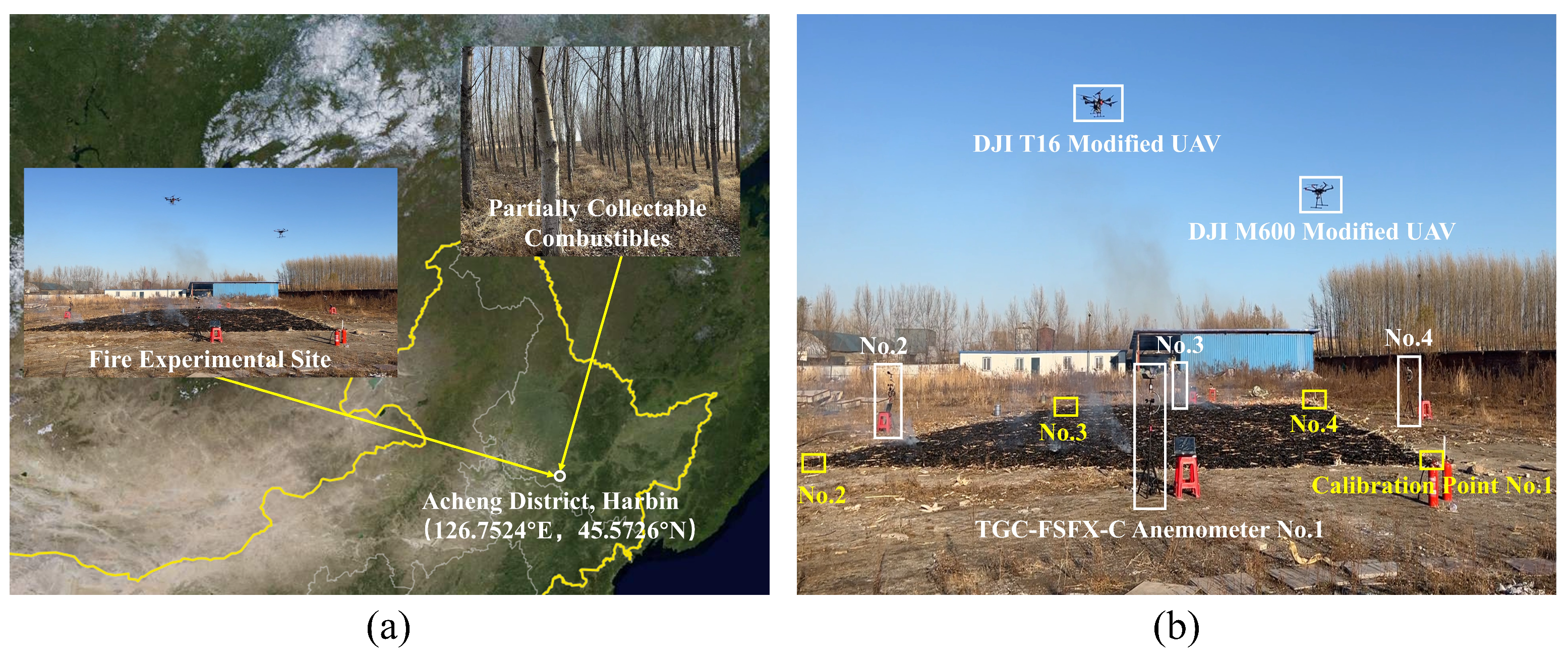
2.1. Small-Scale Ground Fire Experiments

The experimental site for conducting small-scale ground fire experiments was selected in Acheng District, Harbin, China, as shown in Figure 1a. The experimental fire data were collected using a complete set of equipment, some of which are presented in Figure 1b. The DJI M600 UAV equipped with an infrared and visible binocular camera was used to capture the fire spread in real time. Additionally, to ensure the integrity and accuracy of the collected fire spread data, the DJI T16 UAV was deployed to supplement the images captured by the M600 UAV using the same binocular camera. The TGC-FSFX-C anemometers were placed in four directions of the fire site to record real-time wind speed and direction. Considering the limitation of combustible material quantity and enabling perspective transformation [43] for all designed fire experiments, four thermal calibration points were established at 12.8 m east–west (E-W) and 12.8 m north–south (N-S) around the fire site.

We conducted nine small-scale ground fire experiments, and their relevant parameter settings are shown in

Table 1. Relevant parameter settings for nine small-scale ground fire experiments.

Num	Combustibles	Combustible Area	Combustible Weight	Combustible Load	Bed Depth	Moisture Content	Experimental Location
1	Leaf wood	4 × 5 m2	17.895 kg	1.482 kg/m2	5.64 cm	12.2%	126.7524° E, 45.5726° N
2	Leaf wood	6.5 × 7.5 m2	42.86 kg	1.199 kg/m2	6.08 cm	12.1%
3	Leaf wood	6.5 × 7.5 m2	44.275 kg	1.201 kg/m2	6.0 cm	12.5%
4	Leaf wood	8.5 × 8.5 m2	110.345 kg	1.543 kg/m2	5.0 cm	13.9%
5	Conifer	5.5 × 7.3 m2	71.915 kg	1.791 kg/m2	5.0 cm	12.8%
6	Conifer	5.5 × 7 m2	91.06 kg	2.454 kg/m2	7.0 cm	13.1%
7	Sylvestris	7.5 × 7.5 m2	92.565 kg	1.6098 kg/m2	5.0 cm	13.3%
8	Sylvestris	5 × 8 m2	55.6 kg	1.39 kg/m2	6.05 cm	13.0%
9	Poplar leaves	5 × 8 m2	96.7 kg	2.4175 kg/m2	5.0 cm	14.0%

. All the fire experiments were conducted in the same location. In order to ensure the applicability of the proposed model in different scenarios, we collected a variety of combustibles representative of Northeast China, such as conifer, camphor pine, and poplar leaves [44], for experiments. Moreover, we arranged different laying factors, such as the combustible load and bed depth, to simulate diverse environmental variables present during the actual forest fire spread [45]. Each experimental fire continued until all combustible materials had burned out, which typically lasted around 8–10 min depending on the laid combustible area as well as the wind speed and direction at the scene. Throughout the experiments, the UAVs captured image frames of the fire scene continuously while anemometers recorded wind characteristics at the same frame rate. Finally, a total of 4713 fire scene images and the corresponding wind characteristic data were collected.

2.2. Data Preprocessing

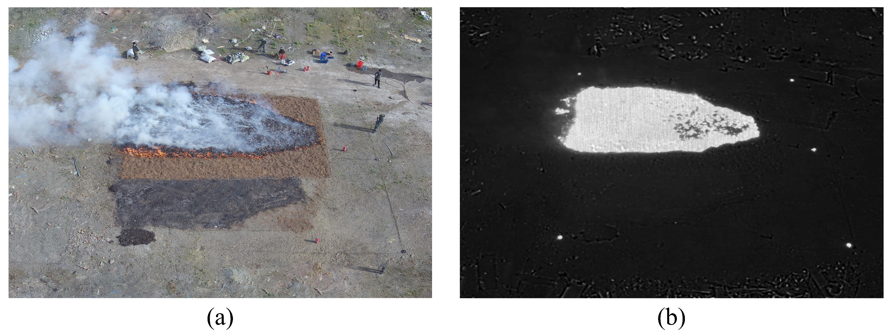
2.2.1. Preprocessing for Combustion Images

There are two types of images collected for each frame, the visible image frame and infrared image frame, as shown in Figure 2. Compared with the visible image frame, the infrared image frame based on thermal imaging technology can avoid the interference caused by a large amount of smoke released by combustion and the surrounding environmental factors in extracting fire scene information [46,47]. Therefore, infrared image frames were selected as combustion images for processing, in which the white pixels represent the burning areas, and the black pixels represent the non-burning areas. Firstly, the median filter method [48] was used to filter the noise of the infrared image frames. Then, the perspective transformation method [49] based on four calibration points was used to convert them into an orthographic projection form. This is because the tilt angle exists between the infrared image taken by the UAV and the ground, and if the original image is directly used for prediction, the predicted result will have a large visual deviation from the actual result. Finally, considering the hardware, the infrared image frames were resized to 128 × 128 pixels. The perspective transformation is shown in Formula (1) [27]:

$$\left[\begin{array}{ccc}{x}^{\prime }\hfill & y^{\prime }\hfill & z^{\prime }\hfill \end{array}\right]=\left[\begin{array}{ccc}u\hfill & vs.\hfill & w\hfill \end{array}\right]\left[\begin{array}{ccc}{a}_{11}\hfill & a_{12}\hfill & a_{13}\hfill \\ a_{21}\hfill & a_{22}\hfill & a_{23}\hfill \\ a_{31}\hfill & a_{32}\hfill & a_{33}\hfill \end{array}\right]$$

(1)

where $a_{3\times 3}$ is the projection matrix, u and v are the original image coordinates, and w is the depth scaling factor, with a value of 1. The image coordinates, x and y, obtained after the perspective transformation, are shown in Formulas (2) and (3) [27]:

$$x=\frac{x^{\prime }}{z^{\prime }}=\frac{a_{11}u+a_{21}v+a_{31}}{a_{13}u+a_{23}v+a_{33}}$$

(2)

$$y=\frac{y^{\prime }}{z^{\prime }}=\frac{a_{12}u+a_{22}v+a_{32}}{a_{13}u+a_{23}v+a_{33}}$$

(3)

2.2.2. Preprocessing for Environmental Variables

The environmental variables are classified as terrain, climate, and combustible variables, which are important for fire spread [50,51,52]. However, due to the limitations in terms of the experimental conditions and scales, the effects of some environmental variables on experimental fire spread were difficult to reflect. Specifically, all of the experimental fires were carried out on the flat ground, meaning that slope, aspect, and elevation did not play a role in experimental fire spread. Furthermore, our experiments were all small-scale fires within a short time period, which led to the effects of temperature, humidity, and combustible moisture content on experimental fire spread being static. Since the laid combustibles were all coniferous, their impact on experimental fire spread was almost identical. Additionally, combustible load and bed depth primarily affected the duration of burning. Only the dynamically changing wind largely guided experimental fires’ speed and direction of spread.

The limited environment variables discussed above may have a negative impact on model training and testing. For instance, employing them for model training may weaken the influence of wind on experimental fire spread while strengthening that of other variables. Thus, we used two preprocessing methods for environmental variables. To process wind speed and direction, we initially computed the average values taken by anemometers in four directions. Then, we transformed these data into pixel images using the min-max scaling algorithm [53] before incorporating them into the combustion images via the channel merging method [54]. For other environmental variables, their effects on the fire spread can be implicitly represented in the dynamic continuous frames of the combustion images, as the combustion images captured by the infrared camera change dynamically over time and have two-dimensional spatial information. Therefore, we intended to enable the model to learn autonomously about their overall impact on fire spread by mining the information implied in the input sequence of consecutive multi-frame combustion images. The min-max scaling algorithm is defined as [55]

$$x^{\ast }=\frac{x-\min \left(x\right)}{\max \left(x\right)-\min \left(x\right)}$$

(4)

where $x^{\ast }$ is the output value, and x is the characteristic value of wind speed or direction.

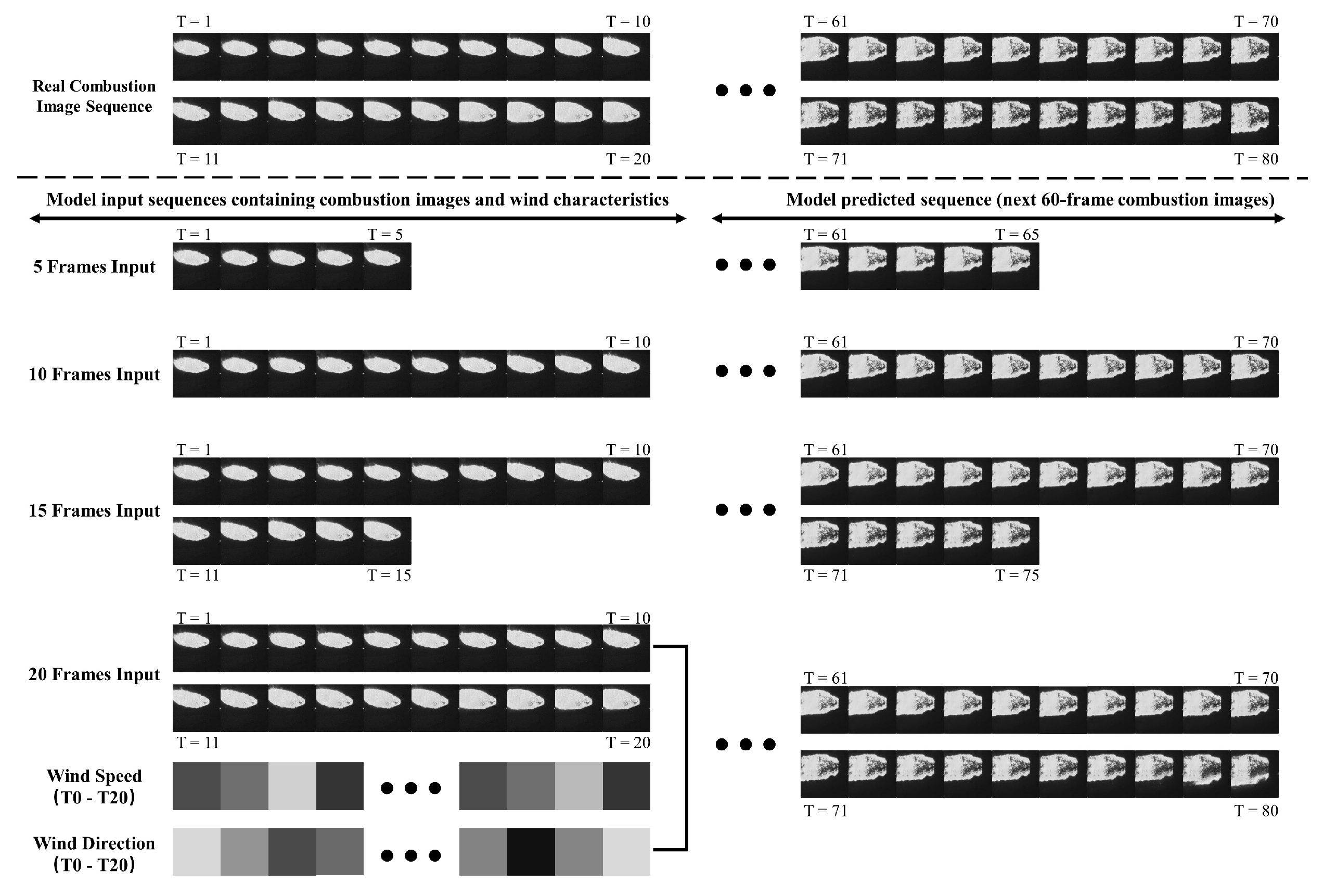
2.3. The Task Definition of Predicting the Combustion Image Sequence

Suppose a fire spreads outward with time in the spatial domain of a $H\times W$ grid consisting of H rows and W columns. In each grid, there are C feature channels that vary over time. Thus, we can set $X_t=R^{C\ast H\ast W}$ to denote the t-th frame in the input sequence of combustion images, where H and W represent the height and width of the input image frames, C represents the number of channels of the input image frames, and R represents the domain of the fire scene features. Based on this, we can introduce the task of predicting the combustion image sequence. Taking the combustion image frames of the previous T timestamps ($X_{in}=\{X_1,X_2,\dots X_T\}$) as the model input, then using the model to predict the combustion image frames of the next K timestamp (${\overline{X}}_{out}=\{{\overline{X}}_{T+1},{\overline{X}}_{T+2},\dots {\overline{X}}_{T+K}\}$), the predicted combustion image frames should be as close as possible to the real combustion image frames ($X_{out}=\{X_{T+1},X_{T+2},\dots X_{T+K}\}$).

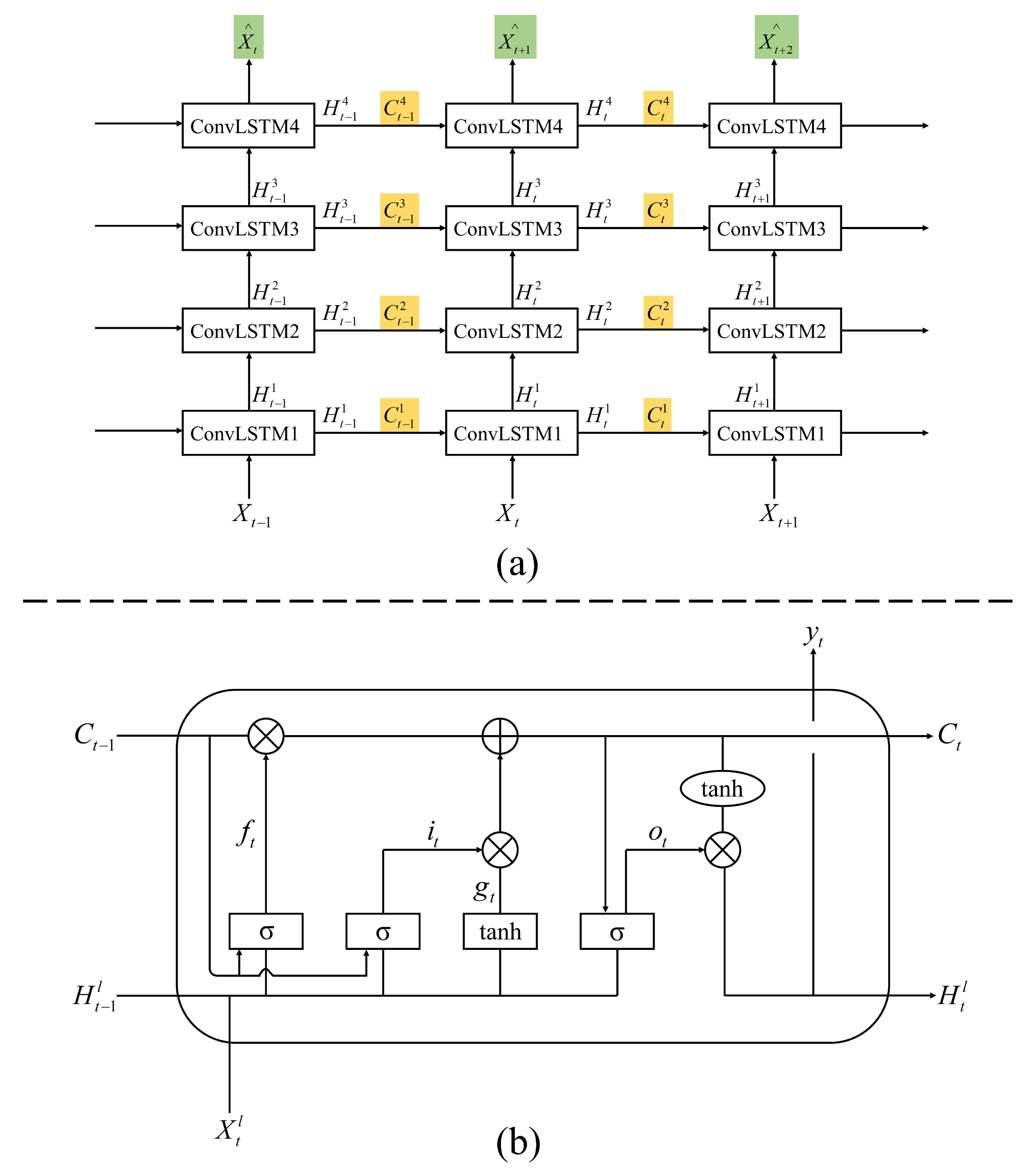
2.4. The State-of-the-Art Spatiotemporal Prediction Models

The spatiotemporal prediction models were selected to solve the defined task, given that fire spread is a dynamic process occurring in both space and time. Two of the main state-of-the-art models are convolutional long short-term memory (ConvLSTM) and predictive recurrent neural network (PredRNN). ConvLSTM [23] has been shown to be effective in predicting fire sequences, and its structure is shown in Figure 3. In this model, the current input state $X_t$ serves as the input for the current layer, together with the hidden state $H_{t-1}$ and the historical memory state $C_{t-1}$ from the previous layer in the horizontal direction. Then, the input is continuously fitted through the upward transmission to obtain advanced image features, and is finally output as the predicted result of the next moment ${\overline{X}}_{t+1}$. The main working principle of ConvLSTM can be described as follows [30,31]:

$$\begin{array}{c}{f}_t=\mathrm{Sigmoid}(W_{xf}\ast X_t+W_{hf}\ast H_{t-1}^l+W_{cf}\otimes C_{t-1}^l+b_f)\hfill \\ i_t=\mathrm{Sigmoid}(W_{xi}\ast X_t+W_{hi}\ast H_{t-1}^l+W_{ci}\otimes C_{t-1}^l+b_f)\hfill \\ g_t=\tanh (W_{xg}\ast X_t+W_{hg}\ast H_{t-1}^l+b_g)\hfill \\ C_t^l=f_t\otimes C_{t-1}^l+i_t\otimes g_t\hfill \\ o_t=\mathrm{Sigmoid}(W_{xo}\ast X_t+W_{ho}\ast H_{t-1}^l+W_{co}\otimes C_t^l+b_o)\hfill \\ H_t^l=o_t\otimes \tanh \left(C_t^l\right)\hfill \end{array}$$

(5)

where ∗ is the convolution operator, and ⊗ is the Hadamard product. $\mathrm{Sigmoid}$ and tanh are activation functions. C and H are the history memory state and hidden state, respectively. $f_t$, $i_t$, $g_t$, and $o_t$ are the forgetting gate, input gate, modulation gate, and output gate, respectively. W is the weight matrix of each input state, memory state, and hidden state. b is the bias parameter corresponding to each control gate.

PredRNN [34] is an improved model based on ConvLSTM, and its structure is shown in Figure 4. Compared with ConvLSTM, it adds a spatiotemporal memory flow, which is highlighted in blue in Figure 4a. This additional flow enables PredRNN to overcome the problem of the lowest layer on the current timestamp, ignoring the topmost information from the previous timestamp, as indicated by the red line in Figure 4a. Furthermore, PredRNN employs both temporal memory flow C and spatiotemporal memory flow M to cope with long-term dynamics and short-term dynamics, respectively. Specifically, it utilizes temporal memory flow to process historical fire features and spatiotemporal memory flow to process the current input combustion image frame and wind characteristics information. This dual approach is more efficient than processing both dynamics simultaneously using only memory units C. According to [34], PredRNN’s primary working principle is described in Formula (6). Both ConvLSTM and PredRNN are used as comparative models for the horizontal comparison experiment, where they are trained and tested using the same method as the proposed model.

$$\begin{array}{c}{f}_t=\mathrm{Sigmoid}\left(W_{xf}\ast X_t+W_{hf}\ast H_{t-1}^l\right)\hfill \\ i_t=\mathrm{Sigmoid}\left(W_{xi}\ast X_t+W_{hi}\ast H_{t-1}^l\right)\hfill \\ g_t=\tanh \left(W_{xg}\ast X_t+W_{hg}\ast H_{t-1}^l\right)\hfill \\ f_t^{\prime }=\mathrm{Sigmoid}\left(W_{xf}^{\prime }\ast X_t+W_{mf}^{\prime }\ast M_t^{l-1}\right)\hfill \\ i_t^{\prime }=\mathrm{Sigmoid}\left(W_{xi}^{\prime }\ast X_t+W_{mi}^{\prime }\ast M_t^{l-1}\right)\hfill \\ g_t^{\prime }=\tanh \left(W_{xg}^{\prime }\ast X_t+W_{mg}^{\prime }\ast M_t^{l-1}\right)\hfill \\ C_t^l=i_t\otimes g_t+f_t\otimes C_{t-1}^l\hfill \\ M_t^l=i_t^{\prime }\otimes g_t^{\prime }+f_t^{\prime }\otimes M_t^{l-1}\hfill \\ o_t=\mathrm{Sigmoid}\left(W_{xo}\ast X_t+W_{ho}\ast H_{t-1}^l+W_{co}\ast C_t^l+W_{mo}\ast M_t^l\right)\hfill \\ H_t^l=o_t\otimes \tanh \left(W_{1\times 1}\ast C_t^l+W_{1\times 1}\ast M_t^l\right)\hfill \end{array}$$

(6)

where M and C represent the spatiotemporal memory state and temporal memory state, respectively. The other parameters are similar to those in Formula (5).

2.5. The Self-Attention Mechanism

Fire spread is a complex long-term phenomenon [32]. Historical fire features, such as the previous burning state and energy released by burning, affect the current burning state and future fire propagation. Therefore, predicting the combustion image sequence is different from other prediction problems, as it involves massive amounts of historical information on temporal and spatial attributes. Once the above spatiotemporal prediction models fail to mine the useful information regarding fire spread increment from these historical fire features, it may lead to an increase in redundant information that can affect the subsequent prediction of the model. To address this issue, the self-attention mechanism [39], which can be regarded as a dynamic feature selection process, is introduced. By incorporating it into the forgetting gate structures of the spatiotemporal prediction model, the model can capture important features from historical fire features by adaptively weighting features. The self-attention mechanism is defined as follows [56]:

$$Y=SoftMax\left(Q{K}^T\right)V$$

(7)

where $SoftMax$ is an activation function, and Q, K, and V represent the query, key, and value, respectively. From the perspective of the spatiotemporal prediction model and in relation to the defined task, Q denotes the current moment’s model input. Its purpose is to score K, which represents historical fire features, in order to obtain an attention score. This score is then multiplied by historical fire features V, which is the same as K, to achieve the self-attention process. The objective of this process is to select the important features associated with the increase in fire spread from massive amounts of historical fire features.

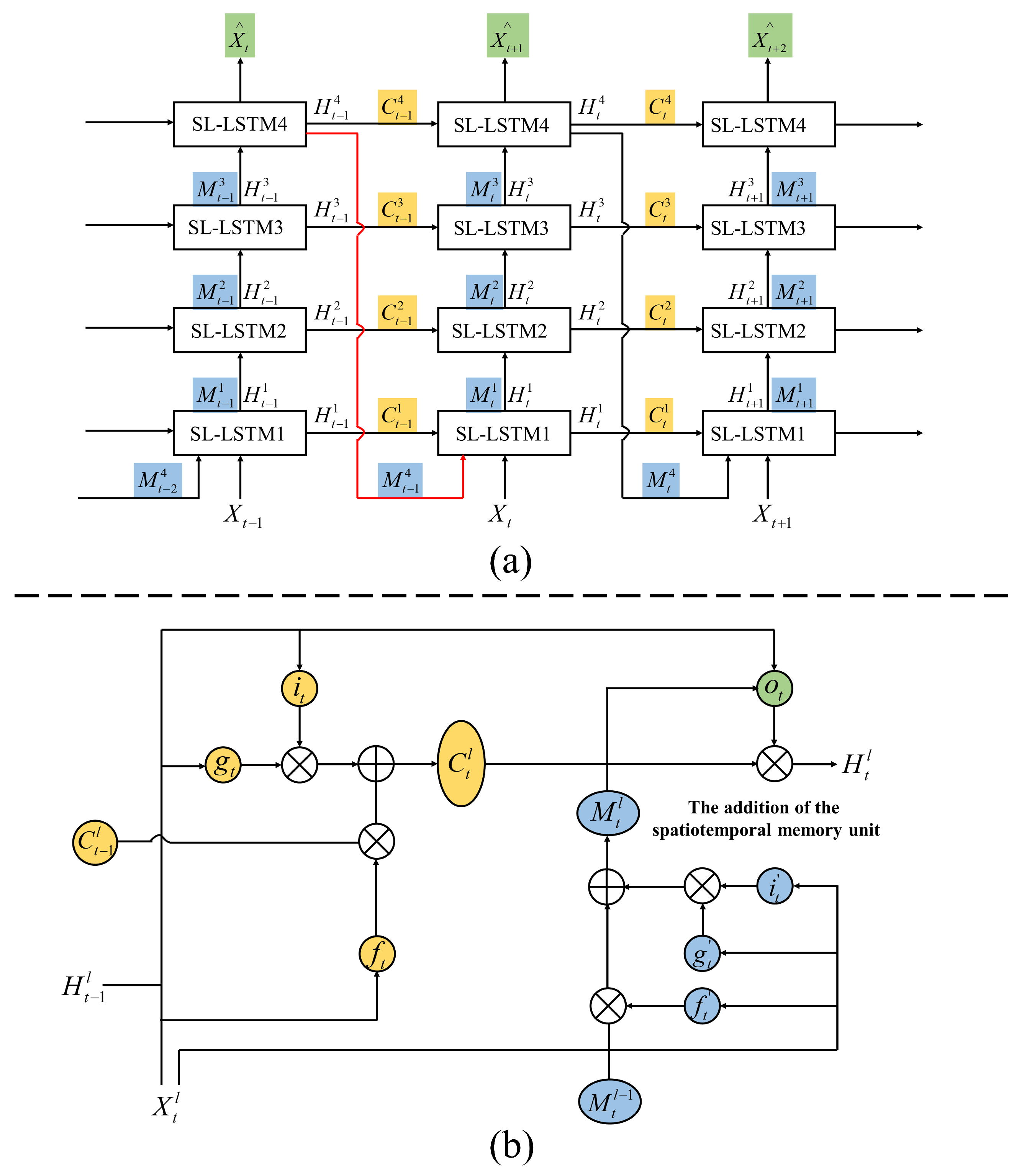
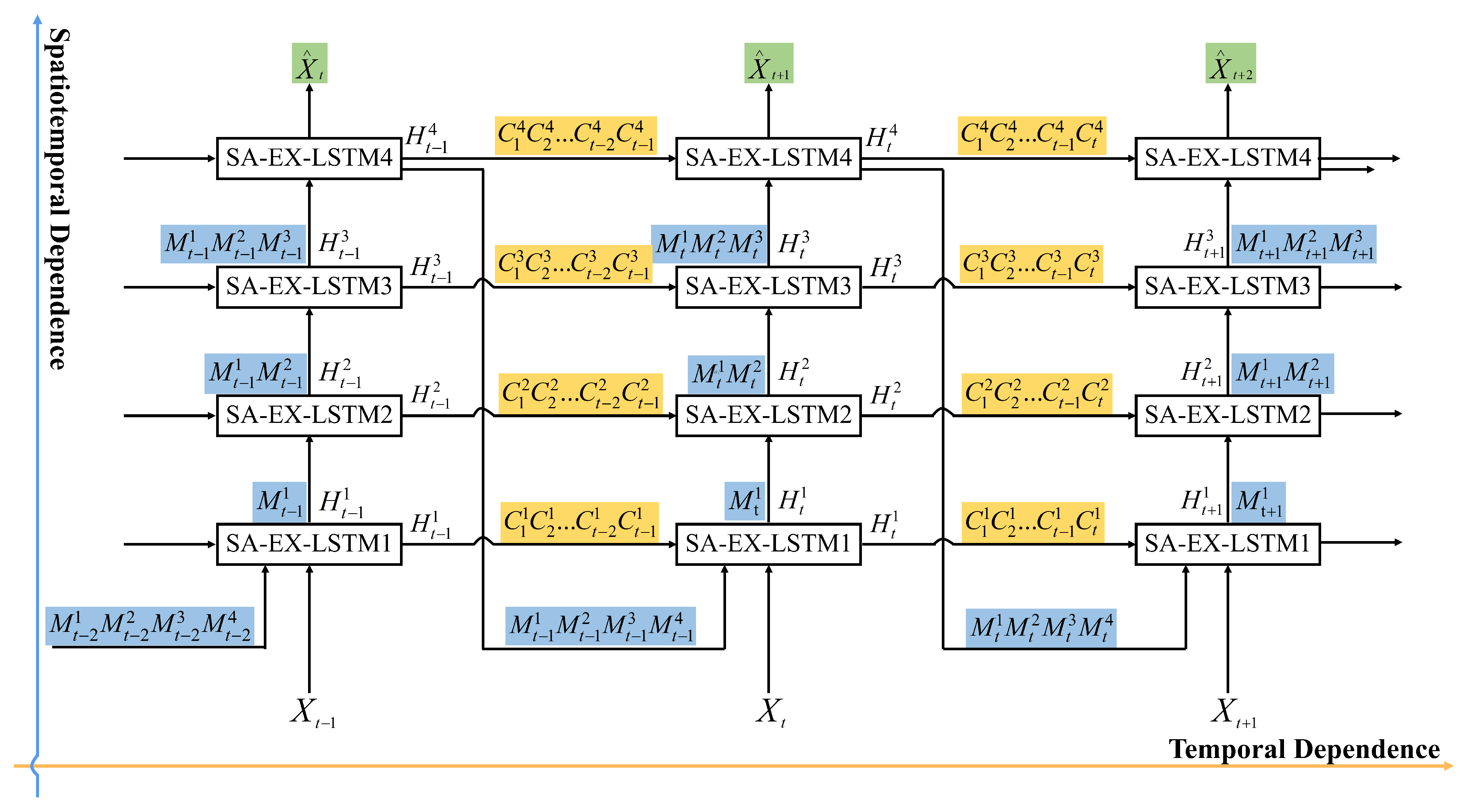
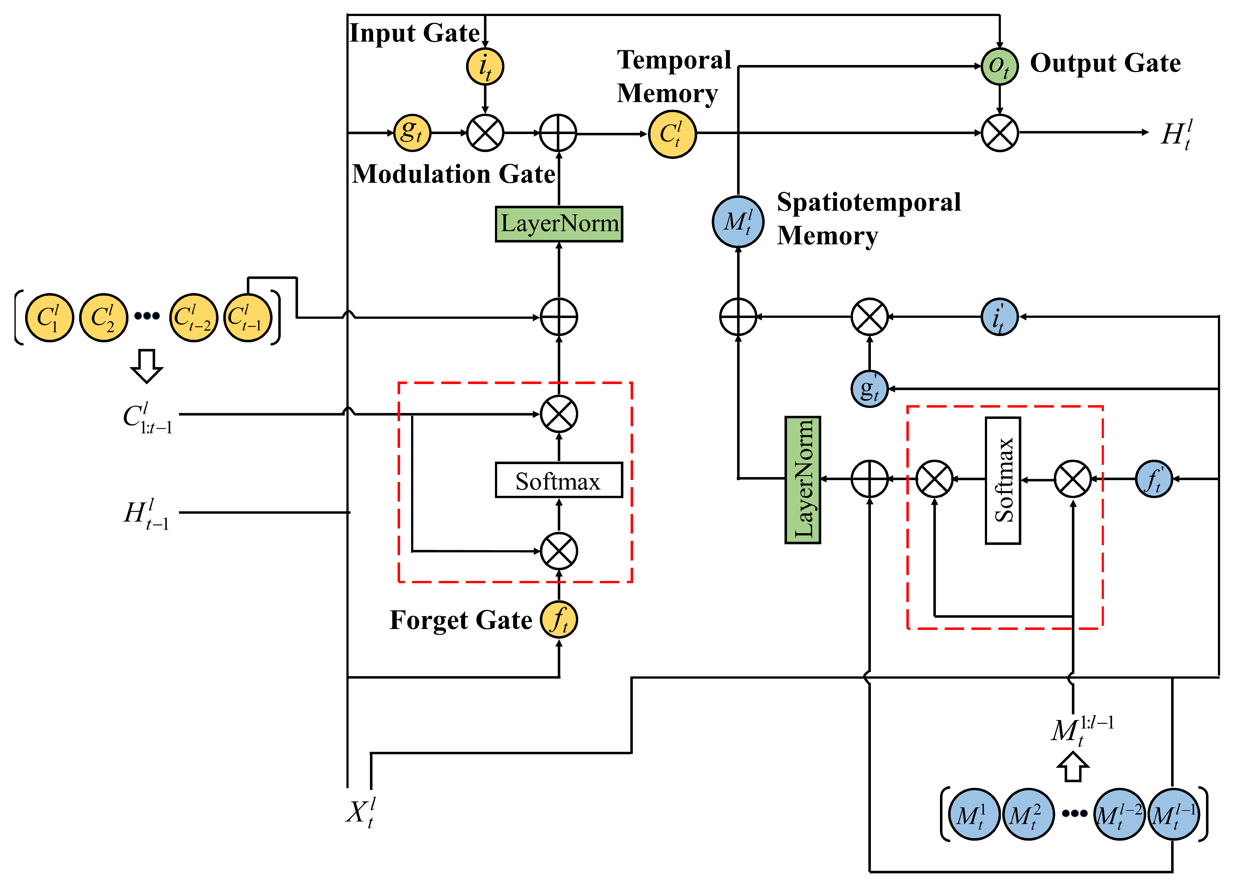
2.6. The Structure of the SA-EX-LSTM

In order to accomplish the defined task, two main points need to be addressed: (1) The model should learn all historical fire feature information stored in the previous layers in as much detail as possible during feature transfer. (2) The model should be able to select the important features that impact the current combustion image prediction from the massive dataset of historical fire feature information. To this end, we proposed an expanded neural network of long short-term memory based on self-attention (SA-EX-LSTM). The model input consists of a series of three-channel images with combustion images, wind speed, and wind direction information. The model output is a subsequent combustion image sequence. The overall network framework of SA-EX-LSTM is shown in Figure 5, and its inner structure is shown in Figure 6.

Concerning point (1), we followed the two-stream mechanism of PredRNN and further improved its original feature transfer rules. When the spatiotemporal memory units M pass vertically upwards, each passing layer will transfer all previous spatiotemporal features ($M_t^{1:l-1}$) containing the current input combustion image and wind characteristic information to the new layer (SA-EX-LSTML), as depicted in the blue section of Figure 5. Similarly, when the temporal memory units C pass horizontally, each passing layer will transfer all previous temporal features ($C_{1:t-1}^l$) containing the historical fire feature information to the new layer, as shown in the yellow section of Figure 5. Based on this new rule, SA-EX-LSTM at each layer can learn more complete historical fire features from improved spatiotemporal and temporal memory flow. Furthermore, the loss of cross-frame historical fire information (the flow of the topmost memory state of the previous timestamp to the lowest of the current timestamp, and the flow of the memory state between parallel layers of adjacent timestamps) can be minimized.

Regarding point (2), we introduced the self-attention mechanism at the location of the spatiotemporal forgetting gate $f_t^{\prime }$ and temporal forgetting gate $f_t$, as shown in the red box section of Figure 6. Taking the role of self-attention in the temporal forgetting gate as an example, it performs parallel computation on historical temporal features ($C_{1:t-1}^l$) and the current model input that has been processed by the temporal forgetting gate. Subsequently, the calculated result is activated by the $SoftMax$ function to obtain the weights of the historical features. Finally, the self-attention mechanism helps the model focus on the important features associated with the increase in fire spread based on these weights. Furthermore, since the combustion state at the $t-1$-th moment has the most significant impact on the prediction of the t-th moment, the temporal memory state of the previous timestamp ($C_{t-1}^l$) was appended to the outcome after the self-attention process was concluded [57]. Likewise, self-attention performed a comparable operation in the spatiotemporal forgetting gate, except the historical temporal features ($C_{1:t-1}^l$) were replaced with historical spatiotemporal features ($M_t^{1:l-1}$). The addition of self-attention mechanisms can help the model better handle the complete historical fire features brought about by improved transfer rules. Moreover, when there is strong interference present within the historical fire features, meaning that many data in these features have little influence on the current combustion image prediction, the effect of the self-attention mechanism will become even more pronounced. In summary, the overall process of each SA-EX-LSTM is as follows:

$$\begin{array}{c}{f}_t=\mathrm{Sigmoid}\left(W_{xf}\ast X_t+W_{hf}\ast H_{t-1}^l+b_f\right)\hfill \\ i_t=\mathrm{Sigmoid}\left(W_{xi}\ast X_t+W_{hi}\ast H_{t-1}^l+b_i\right)\hfill \\ g_t=\tanh \left(W_{xg}\ast X_t+W_{hg}\ast H_{t-1}^l+b_g\right)\hfill \\ f_t^{\prime }=\mathrm{Sigmoid}\left(W_{xf}^{\prime }\ast X_t+W_{mf}^{\prime }\ast M_t^{l-1}+b_f^{\prime }\right)\hfill \\ i_t^{\prime }=\mathrm{Sigmoid}\left(W_{xi}^{\prime }\ast X_t+W_{mi}^{\prime }\ast M_t^{l-1}+b_i^{\prime }\right)\hfill \\ g_t^{\prime }=\tanh \left(W_{xg}^{\prime }\ast X_g+W_{mg}^{\prime }\ast M_t^{l-1}+b_g^{\prime }\right)\hfill \\ SA\left(f_t,C_{1:t-1}^l\right)=\mathit{SoftMax}\left(f_t·{\left(C_{1:t-1}^l\right)}^T\right)·C_{1:t-1}^l\hfill \\ C_t^l=i_t\otimes g_t+\mathrm{LayerNorm}\left(C_{t-1}^l+SA\left(f_t,C_{1:t-1}^l\right)\right)\hfill \\ SA\left(f_t,M_t^{1:l-1}\right)=\mathit{SoftMax}\left(f_t·{\left(M_t^{1:l-1}\right)}^T\right)·M_t^{1:l-1}\hfill \\ M_t^l=i_t^{\prime }\otimes g_t^{\prime }+\mathrm{LayerNorm}\left(M_t^{l-1}+SA\left(f_t,M_t^{1:l-1}\right)\right)\hfill \\ o_t=\mathrm{Sigmoid}\left(W_{xo}\ast X_t+W_{ho}\ast H_{t-1}^l+W_{co}\ast C_t^l+W_{mo}\ast M_t^l+b_o\right)\hfill \\ H_t^l=o_t\otimes \tanh \left(W_{1\times 1}\ast C_t^l+W_{1\times 1}\ast M_t^l\right)\hfill \end{array}$$

(8)

where ∗ is the convolution operator, and · and ⊗ denote the matrix product and the Hadamard product, respectively. $f_t$, $i_t$, and $g_t$ represent the forgetting gate, the input gate, and the modulation gate of the temporal memory module, respectively. $f_t^{\prime }$, $i_t^{\prime }$, and $g_t^{\prime }$ delegate the forgetting gate, the input gate, and the modulation gate of the spatiotemporal memory module, respectively. W and b denote the weights and biases of each control gate unit. $SA$ is the self-attention transition unit. $C_t^l$ is the l-level temporal memory state of the t-th timestamp, and $M_t^l$ is the l-level spatiotemporal memory state of the t-th timestamp. $C_{1:t-1}^l$ denote all the temporal memory states from the first timestamp to the $t-1$-th timestamp of layer l. $M_t^{1:l-1}$ delegate all the spatiotemporal memory states from the first level to the $l-1$-th level within the t-th timestamp. $H_t^l$ denotes the l-level layer hidden state of the t-th timestamp. $o_t$ is the output gate that couples $C_t^l$ and $M_t^l$. $W_{1\times 1}$ is a 1 × 1 reduced-dimensions convolutional layer. Moreover, LayerNorm [58] is used to ensure the stability of data feature distribution, and accelerate model convergence.

The architecture of SA-EX-LSTM was built by PyTorch, and all the experiments were conducted on an AMD R7-5800H 4.40 GHz processor with 16 GB RAM and an NVIDIA GTX 3060 graphics card. The batch size [59], which is the number of data points selected for one round of training, was set to 2. To evaluate the difference between the predicted and real results to guide the model training, the mean square error (MSE) [60] was selected as the loss function, which is a commonly used measure in regression problems. Another important hyperparameter in model training is the learning rate [61], which determines whether the loss function can converge to the minimum and how to converge to the minimum. The Adam optimizer [62] was selected to allow the model to automatically adjust the learning rate while training, and its initial value was set to $1\times {10}^{-3}$. The data from eight experimental fires (4361 pairs of combustion images and their corresponding wind speed and direction) were used for model training, and the data from one experimental fire (352 pairs of combustion images and their corresponding wind speed and direction) were used for model testing.

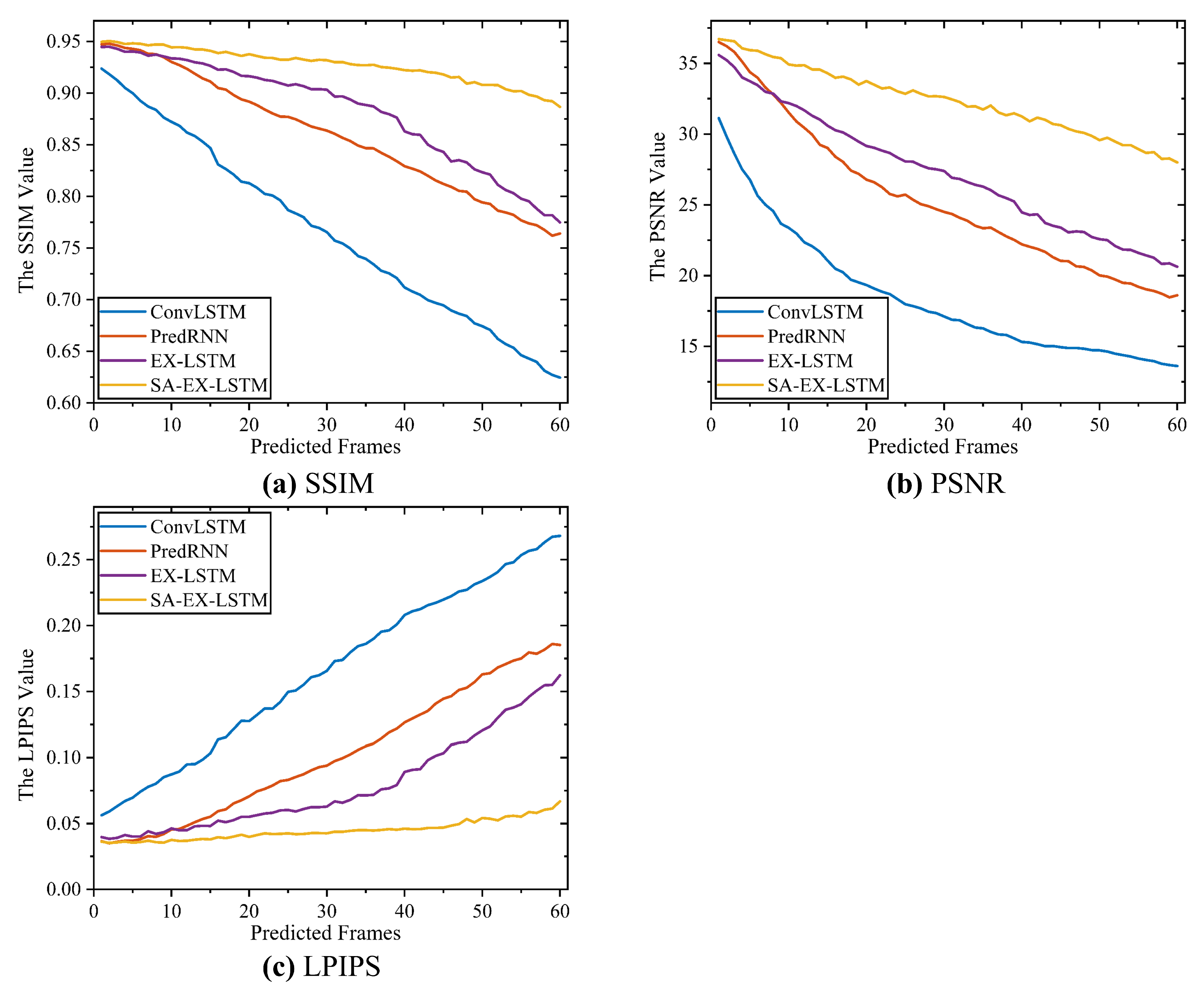
2.7. Performance Metrics

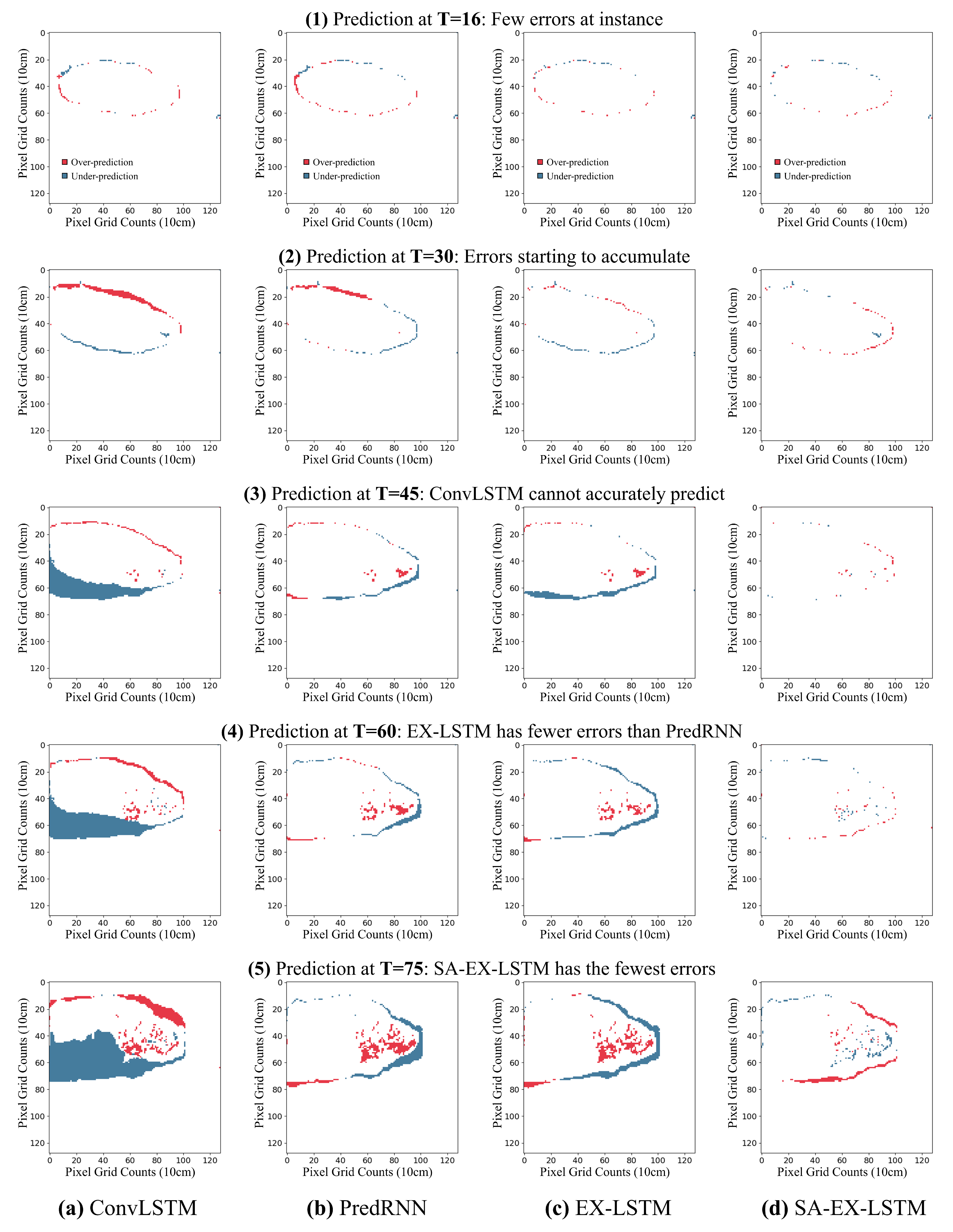
In order to comprehensively evaluate the model’s predicted performance, several common metrics in the image generation task were selected. Structural similarity (SSIM) [63] was used to measure the similarity between predicted and real combustion images. It is defined as follows [64]:

$$\mathrm{SSIM}(X,\overline{X})=\frac{\left(2{\mu }_X{\mu }_{\overline{X}}+c_1\right)+\left(2{\sigma }_{X\overline{X}}+c_2\right)}{\left({\mu }_X^2+{\mu }_{\overline{X}}^2++c_1\right)\left({\sigma }_X^2+{\sigma }_{\overline{X}}^2++c_2\right)}$$

(9)

where X and $\overline{X}$ represent the predicted and real combustion image frame, respectively. ${\sigma }^2$ is the variance of the image. $\mu$ is the average of the image. ${\sigma }_{X\overline{X}}$ is the covariance of two images. c is the bias constant.

The peak signal to noise ratio (PSNR) [65] was used to measure the noise of the predicted combustion images, i.e., the presence of some white pixels (predicting a fire in that raster) in the surrounding environment of the predicted combustion image. It is defined as follows [66]:

$$\begin{array}{c}MSE=\frac{1}{H\times W}{\sum }_{i=1}^H{\sum }_{j=1}^W{[X(i,j)-\overline{X}(i,j)]}^2\hfill \\ PSNR=10\times \lg \left[\frac{{\left(2^n-1\right)}^2}{MSE}\right]\hfill \end{array}$$

(10)

where $MSE$ denotes the mean square error of X and $\overline{X}$. H and W represent the height and width of the image, respectively.

Learned perceptual image patch similarity (LPIPS) [67] was used as one of the performance metrics of the model. Compared with SSIM and PSNR, LPIPS can better explain the slight gap between predicted and real combustion images. Among the above three metrics, the larger the SSIM and PSNR values, the smaller the LPIPS value, and the better the model-predicted performance.

3. Results

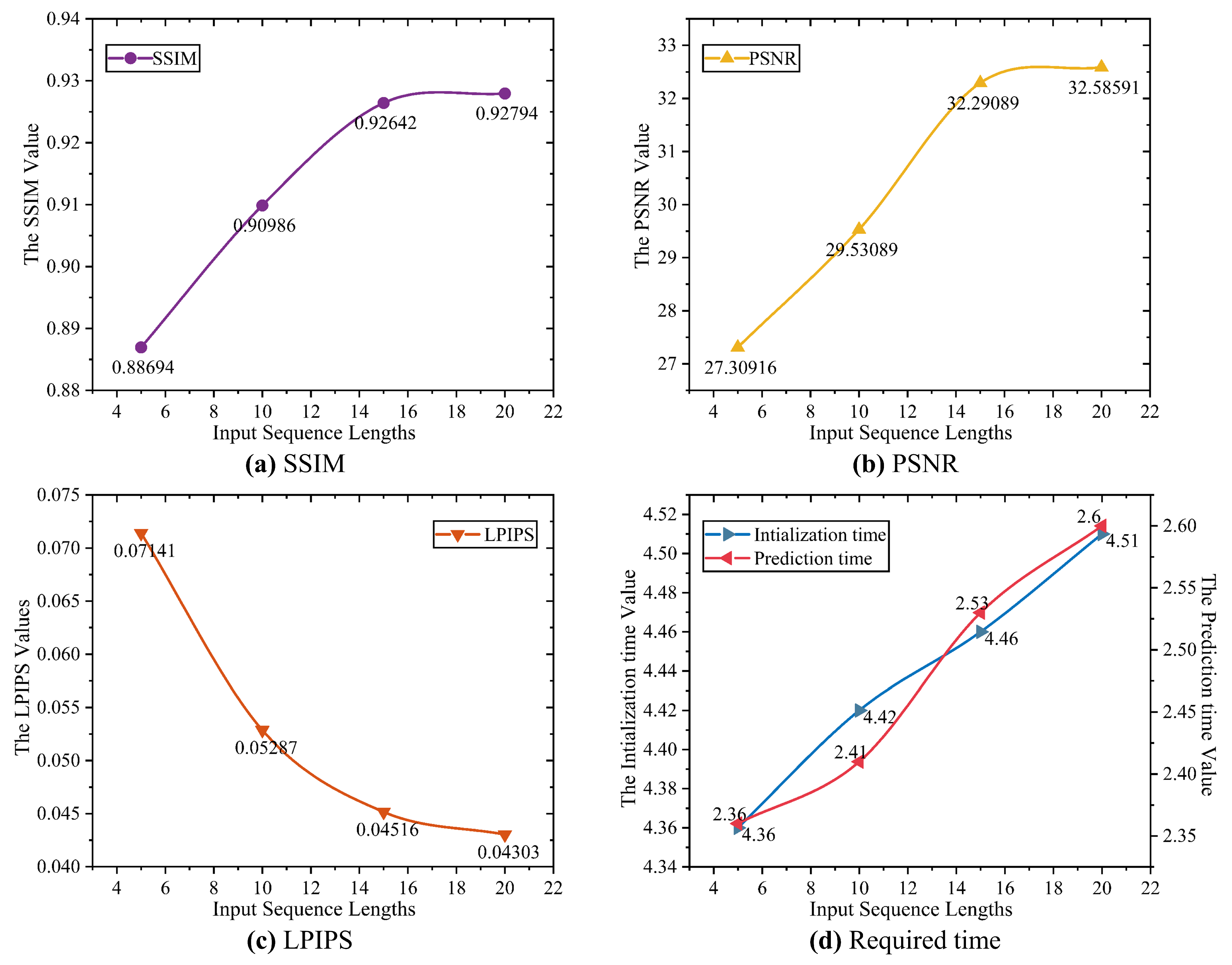
The Influence of Different Input Sequence Lengths on Model Prediction

Different input sequence lengths can impact the predicted performance of the model, as they imply different amounts of historical fire information. To account for this, we used combustion image sequences in sets of five, ten, fifteen, and twenty frames, with corresponding wind characteristics, as inputs to the model. Subsequently, we predicted the combustion image sequence for the following sixty frames beginning from the last frame of the input. The partial results of the predicted fire sequences in the testing set are shown in Figure 7. In addition, to determine the optimal number of input frames, we evaluated the model’s prediction performance and time required to predict the 60-frame sequence in the whole testing set, and used a spline curve to fit these data. The fitting results are presented in Figure 8.

The SA-EX-LSTM was compared with the state-of-the-art spatiotemporal prediction models, including ConvLSTM and PredRNN, to assess its predicted performance. Considering the two improvements made in the proposed model, the expended LSTM model, EX-LSTM (the SA-EX-LSTM model without self-attention mechanism), was also used as a comparison model. The aforementioned models were applied to the testing set sequences by inputting 15-frame combustion images and their corresponding wind characteristics to predict future 60-frame combustion images. The predicted results from multiple moments were selected, and their predicted errors are visualized in Figure 9. Red pixels indicate over-predicted pixels (there is no fire in the grid, but the model predicts that there is a fire), and blue pixels represent under-predicted pixels (fire exists in the grid, but no fire is predicted). In addition, we quantified the performance variation of these models across the entire continuous prediction period for the testing set sequences, as shown in Figure 10.

4. Discussion

Changes in input sequence length can affect the predictive performance and the prediction time of the model [68,69], as demonstrated in Figure 7 and Figure 8. With the input frames increasing, the predicted performance of SA-EX-LSTM gradually improves. This phenomenon is because more input frames provide more historical information on fire features, allowing the model to better learn the process and trend of fire spread. This effect is particularly significant when the model input frames are small. By accumulating input frames from 5 to 20, the SSIM and PSNR increase by 0.041 and 5.27675, and the LPIPS decreases by 0.02838. Furthermore, the growth rate of the model’s predicted performance begins to slow down after the input frames exceed 15 frames, as historical fire feature information from too early is less relevant to the current fire spread. Inputting too many previous combustion images can lead to information redundancy, which interferes with model prediction [70]. Although the increase in input frames is beneficial to the model’s predicted performance, it is also accompanied by an increase in initialization time and prediction time, thereby impacting model efficiency [71,72]. As the input frames accumulate from 5 to 20, the prediction time of the model increases by 10.17%, with no significant decrease in growth rate. Therefore, it is not feasible to blindly increase the input frames only for the model’s predicted performance, and the predicted efficiency should also be taken into consideration. In order to strike a balance between the two, we ultimately select 15 consecutive frames of combustion images as the input for SA-EX-LSTM.

The predicted results of SA-EX-LSTM and its comparative models at multiple equidistant moments can be clearly seen in Figure 9. All of the models can predict the next one-frame combustion image well. However, as the number of predicted time frames increases, some models face difficulty in maintaining their predictive performance due to the accumulation of prediction errors in pixels [73]. ConvLSTM [31] shows a significant decrease in predictive performance in the mid-term of the predicted sequence (continuously predicting 30 frames, T = 45) due to the inadequate processing of historical fire features [33]. In comparison, PredRNN [34] and EX-LSTM still have a better-predicted performance in the mid-to-late term of the predicted sequence (continuously predicting 45 frames, T = 60). This result shows that the addition of spatiotemporal memory units to the two models helps the original memory units share the processing pressure for short-term dynamics (the current combustion image and wind characteristics information) [34]. Only SA-EX-LSTM maintains good predicted performance in the late term of the predicted sequence (continuously predicting 60 frames, T = 75).

Figure 10 presents the quantitative results of the continuous predicted performance using the models discussed above. SA-EX-LSTM, represented by the yellow line, consistently exhibits the highest predicted performance and stability, thanks to the improved feature transfer rules and the integrated self-attention mechanism [39]. During the prediction of the next 60-frame combustion images, SA-EX-LSTM achieves an SSIM over 0.88669 and PSNR above 27.99768 while keeping LPIPS below 0.06692 [74]. Furthermore, EX-LSTM is used as a comparative model for an ablation experiment [75] to more accurately describe the influence of the aforementioned improvements. By improving the feature transfer rules, EX-LSTM can learn more complete historical fire features to guide the model prediction, resulting in superior predicted performance compared to PredRNN throughout the predictive process. However, it should be noted that ConvLSTM’s predicted performance decreases faster than PredRNN after the mid-term of the prediction sequence due to the improved rules introducing excessive historical fire information, which the model cannot use correctly. The self-attention mechanism can address this issue by being integrated into the forgetting gates of the model, thereby helping the model select the important features associated with the increase in fire spread and suppress redundant features from massive datasets of historical fire features [35]. The improvement in the model-predicted performance by the self-attention mechanism is evident in the quantified results of SA-EX-LSTM and EX-LSTM.

Although there are some limitations to the experiment, they have minimal impact on the overall evaluation of the proposed model. The improved transfer rules and integrated self-attention mechanism increase model complexity and prediction time, but this is offset by the improvement in predicted performance. Given that SA-EX-LSTM only takes 2.6 s to predict the testing set sequence (a total of ten 60-frame sequences), we did not consider its gap with PredRNN and ConvLSTM in terms of prediction time. Within the fire margin of the infrared image, there exist areas that have been fully burned and appear as black pixels in Figure 2b. Since we did not fill the areas, the models in this paper classify them as combustible. This may result in a decrease in the model’s predicted performance. Moreover, although our evaluation of the proposed models was limited to predicting 60-frame (60 s) combustion images, the model can be applied to longer-duration fires by adjusting the frame rate captured by the infrared camera [76]. Our proposed model predicts the combustion image sequence based on wind characteristics and achieves good predicted performance in small-scale experimental fires, positively impacting the application of spatiotemporal prediction models in fire spread. In addition, all of the models in the study were trained and tested using infrared images taken by the UAVs, providing theoretical support for the application of UAVs in fighting forest fires.

5. Conclusions

In order to accurately predict combustion image sequences to better guide forest fire management, we proposed an expanded neural network of LSTM based on self-attention (SA-EX-LSTM). The proposed model has two improvements over the previous spatiotemporal prediction model. First, it incorporates a more detailed feature transfer rule, enabling the model to learn more complete historical fire features. Second, the self-attention mechanisms are incorporated into the temporal and spatiotemporal forgetting gates to help the model select the important features associated with the increase in fire spread. We conducted a total of nine fire experiments and used these data to train and test the proposed model. Upon analyzing the results, we draw the following conclusions:

(1) The input sequence length is a critical variable for the model, as it influences the model prediction through the embedded historical fire information. As the input frames increase, the model’s predicted performance improves, but this is also accompanied by an increase in the initialization time and prediction time. For the dataset used in the study, the optimal value is 15 frames.

(2) In comparison to state-of-the-art models, including ConvLSTM [31], and PredRNN [34], the proposed model consistently exhibits the highest predicted performance and stability when predicting the subsequent 60-frame combustion images. Its SSIM and PSNR can reach above 0.88669 and 27.99768, respectively, while maintaining an LPIPS value below 0.06692. Furthermore, ablation experiment results indicate that the improved feature transfer rules and the integrated self-attention [39] are both indispensable. By processing the historical fire features, they can improve the predicted performance of the proposed model to varying degrees.

(3) The proposed model predicts the combustion image sequence based on wind characteristics and achieves good predicted performance in small-scale experimental fires, positively impacting the application of spatiotemporal prediction models in the field of fire spread prediction. In addition, all of the models in this study were trained and tested using infrared images taken by the UAVs, providing theoretical support for the application of UAVs in fighting forest fires.

References

1. Zhao, F.; Shu, L.F.; Zhou, R.L. A review of wildland fire spread modelling. World For. Res. 2017, 30, 46–50. [Google Scholar]
2. Zong, X.Z.; Tain, X.R. Research progress in forest fire behavior and suppression technology. World For. Res. 2019, 32, 31–36. [Google Scholar]
3. San José, R.; Pérez, J.L.; González, R.M. Analysis of fire behaviour simulations over Spain with WRF-FIRE. Int. J. Environ. Pollut. 2014, 55, 148–156. [Google Scholar] [CrossRef]
4. Cruz, M.G.; Alexander, M.E. Modelling the rate of fire spread and uncertainty associated with the onset and propagation of crown fires in conifer forest stands. Int. J. Wildland Fire 2017, 26, 413–426. [Google Scholar] [CrossRef]
5. Fons, W.L. Analysis of fire spread in light forest fuels. J. Agric. Res. 1946, 72, 93–121. [Google Scholar]
6. Albini, F.A. A model for fire spread in wildland fuels by-radiation. Combust. Sci. Technol. 1985, 42, 229–258. [Google Scholar] [CrossRef]
7. Wang, X.; Wotton, B.M.; Cantin, A.S. cffdrs: An R package for the Canadian forest fire danger rating system. Ecol. Process. 2017, 6, 5. [Google Scholar] [CrossRef]
8. Leonard, S. Predicting sustained fire spread in Tasmanian native grasslands. Environ. Manag. 2009, 44, 430–440. [Google Scholar] [CrossRef]
9. Rothermel, R.C. A Mathematical Model for Predicting Fire Spread in Wildland Fuels; Intermountain Forest & Range Experiment Station, Forest Service, US Department of Agriculture: Washington, DC, USA, 1972.
10. Finney, M.A. Fire Area Simulator–Model Development and Evaluation; US Department of Agriculture, Forest Service, Rocky Mountain Research Station: Washington, DC, USA, 1998.
11. Zhang, F.; Xie, X. An Improved Forest Fire Spread Model and Its Realization. Geomat. Spat. Inf. Technol. 2012, 35, 50–53. [Google Scholar]
12. Sullivan, A.L. A review of wildland fire spread modelling, 1990–present, 1: Physical and quasi-physical models. arXiv 2007, arXiv:0706.3074. [Google Scholar]
13. Sullivan, A.L. Wildland surface fire spread modelling, 1990–2007. 2: Empirical and quasi-empirical models. Int. J. Wildland Fire 2009, 18, 369–386. [Google Scholar] [CrossRef] [Green Version]
14. Andrews, P.L.; Cruz, M.G.; Rothermel, R.C. Examination of the wind speed limit function in the Rothermel surface fire spread model. Int. J. Wildland Fire 2013, 22, 959–969. [Google Scholar] [CrossRef]
15. Andrews, P.L. The Rothermel Surface Fire Spread Model and Associated Developments: A Comprehensive Explanation; United States Department of Agriculture, Forest Service, Rocky Mountain Research Station: Washington, DC, USA, 2018.
16. Li, X.; Zhang, M.; Zhang, S. Simulating forest fire spread with cellular automation driven by a LSTM based speed model. Fire 2022, 5, 13. [Google Scholar] [CrossRef]
17. Sakr, G.E.; Elhajj, I.H.; Mitri, G. Artificial intelligence for forest fire prediction. In Proceedings of the 2010 IEEE/ASME International Conference on Advanced Intelligent Mechatronics, Montreal, QC, Canada, 6–9 July 2010; pp. 1311–1316. [Google Scholar]
18. Castelli, M.; Vanneschi, L.; Popovič, A. Predicting burned areas of forest fires: An artificial intelligence approach. Fire Ecol. 2015, 11, 106–118. [Google Scholar] [CrossRef]
19. Wu, Z.; Li, M.; Wang, B. Using artificial intelligence to estimate the probability of forest fires in Heilongjiang, northeast China. Remote Sens. 2021, 13, 1813. [Google Scholar] [CrossRef]
20. Hodges, J.L.; Lattimer, B.Y. Wildland fire spread modeling using convolutional neural networks. Fire Technol. 2019, 55, 2115–2142. [Google Scholar] [CrossRef]
21. Wu, Z.; Wang, B.; Li, M. Simulation of forest fire spread based on artificial intelligence. Ecol. Indic. 2022, 136, 108653. [Google Scholar] [CrossRef]
22. Marjani, M.; Mesgari, M.S. The Large-Scale Wildfire Spread Prediction Using a Multi-Kernel Convolutional Neural Network. ISPRS Ann. Photogramm. Remote Sens. Spat. Inf. Sci. 2023, 10, 483–488. [Google Scholar] [CrossRef]
23. Singh, K.R.; Neethu, K.P.; Madhurekaa, K. Parallel SVM model for forest fire prediction. Soft Comput. Lett. 2021, 3, 100014. [Google Scholar] [CrossRef]
24. Casallas, A.; Jiménez-Saenz, C.; Torres, V. Design of a forest fire early alert system through a deep 3D-CNN structure and a WRF-CNN bias correction. Sensors 2022, 22, 8790. [Google Scholar] [CrossRef]
25. Zhang, G.; Wang, M.; Liu, K. Forest fire susceptibility modeling using a convolutional neural network for Yunnan province of China. Int. J. Disaster Risk Sci. 2019, 10, 386–403. [Google Scholar] [CrossRef] [Green Version]
26. Allaire, F.; Mallet, V.; Filippi, J.B. Emulation of wildland fire spread simulation using deep learning. Neural Netw. 2021, 141, 184–198. [Google Scholar] [CrossRef] [PubMed]
27. Li, X.; Lin, C.; Zhang, M. Predicting the rate of forest fire spread toward any directions based on a CNN model considering the correlations of input variables. J. For. Res. 2023, 28, 111–119. [Google Scholar] [CrossRef]
28. Cheng, T.; Wang, J. Integrated spatio-temporal data mining for forest fire prediction. Trans. GIS 2008, 12, 591–611. [Google Scholar] [CrossRef]
29. Li, D.; Cova, T.J. Dennison, P.E. Setting wildfire evacuation triggers by coupling fire and traffic simulation models: A spatiotemporal GIS approach. Fire Technol. 2019, 55, 617–642. [Google Scholar] [CrossRef]
30. Shi, X.; Chen, Z.; Wang, H. Convolutional LSTM network: A machine learning approach for precipitation nowcasting. Adv. Neural Inf. Process. Syst. 2015, 28, 802–810. [Google Scholar]
31. Burge, J.; Bonanni, M.; Ihme, M. Convolutional LSTM neural networks for modeling wildland fire dynamics. arXiv 2020, arXiv:2012.06679. [Google Scholar]
32. Papadopoulos, G.D.; Pavlidou, F.N. A comparative review on wildfire simulators. IEEE Syst. J. 2011, 5, 233–243. [Google Scholar] [CrossRef]
33. Su, J.; Byeon, W.; Kossaifi, J. Convolutional tensor-train lstm for spatio-temporal learning. Adv. Neural Inf. Process. Syst. 2020, 33, 13714–13726. [Google Scholar]
34. Wang, Y.; Wu, H.; Zhang, J. Predrnn: A recurrent neural network for spatiotemporal predictive learning. IEEE Trans. Pattern Anal. Mach. Intell. 2022, 4, 2208–2225. [Google Scholar] [CrossRef]
35. Guo, M.H.; Xu, T.X.; Liu, J.J. Attention mechanisms in computer vision: A survey. Comput. Vis. Media 2022, 8, 331–368. [Google Scholar] [CrossRef]
36. Cao, Y.; Yang, F.; Tang, Q. An attention enhanced bidirectional LSTM for early forest fire smoke recognition. IEEE Access 2019, 7, 154732–154742. [Google Scholar] [CrossRef]
37. Li, Z.; Huang, Y.; Li, X. Wildland fire burned areas prediction using long short-term memory neural network with attention mechanism. Fire Technol. 2021, 57, 1–23. [Google Scholar] [CrossRef]
38. Majid, S.; Alenezi, F.; Masood, S. Attention based CNN model for fire detection and localization in real-world images. Expert Syst. Appl. 2022, 189, 116114. [Google Scholar] [CrossRef]
39. Vaswani, A.; Shazeer, N.; Parmar, N. Attention is all you need. Adv. Neural Inf. Process. Syst. 2017, 30, 6000–6010. [Google Scholar]
40. Zhao, H.; Jia, J.; Koltun, V. Exploring self-attention for image recognition. In Proceedings of the IEEE/CVF Conference on Computer Vision and Pattern Recognition, Seattle, WA, USA, 13–19 June 2020; pp. 10076–10085. [Google Scholar]
41. Zhang, H.; Goodfellow, I.; Metaxas, D. Self-attention generative adversarial networks. In Proceedings of the International Conference on Machine Learning, Beach, CA, USA, 10–15 June 2019; pp. 7354–7363. [Google Scholar]
42. Wang, S.; Li, B.Z.; Khabsa, M. Linformer: Self-attention with linear complexity. arXiv 2020, arXiv:2006.04768. [Google Scholar]
43. Mezirow, J. Perspective transformation. Adult Educ. 1978, 28, 100–110. [Google Scholar] [CrossRef]
44. Wu, B.; Mu, C.; Zhao, J. Effects on carbon sources and sinks from conversion of over-mature forest to major secondary forests and korean pine plantation in Northeast China. Sustainability 2019, 11, 4232. [Google Scholar] [CrossRef] [Green Version]
45. Li, X.; Gao, H.; Zhang, M. Prediction of Forest fire spread rate using UAV images and an LSTM model considering the interaction between fire and wind. Remote Sens. 2021, 13, 4325. [Google Scholar] [CrossRef]
46. Vollmer, M. Infrared thermal imaging. In Computer Vision: A Reference Guide; Springer International: Cham, Switzerlnad, 2021; pp. 666–670. [Google Scholar]
47. Ciprián-Sánchez, J.F.; Ochoa-Ruiz, G.; González-Mendoza, M. Assessing the applicability of Deep Learning-based visible-infrared fusion methods for fire imagery. arXiv 2021, arXiv:2101.11745v2. [Google Scholar]
48. Pei, Z.; Tong, Q.; Wang, L. A median filter method for image noise variance estimation. In Proceedings of the 2010 Second, International Conference on Information Technology and Computer Science, Kiev, Ukraine, 24–25 July 2010; pp. 13–16. [Google Scholar]
49. Zhang, J.; Zhang, J.; Chen, B. A perspective transformation method based on computer vision. In Proceedings of the 2020 IEEE International Conference on Artificial Intelligence and Computer Applications (ICAICA), Dalian, China, 27–29 June 2020; pp. 765–768. [Google Scholar]
50. Cary, G.J.; Keane, R.E.; Gardner, R.H. Comparison of the sensitivity of landscape-fire-succession models to variation in terrain, fuel pattern, climate and weather. Landsc. Ecol. 2006, 21, 121–137. [Google Scholar] [CrossRef]
51. Guo, F.; Su, Z.; Wang, G. Understanding fire drivers and relative impacts in different Chinese forest ecosystems. Sci. Total. Environ. 2017, 605, 411–425. [Google Scholar] [CrossRef] [PubMed]
52. Coop, J.D.; Parks, S.A.; Stevens-Rumann, C.S. Extreme fire spread events and area burned under recent and future climate in the western USA. Glob. Ecol. Biogeogr. 2022, 31, 1949–1959. [Google Scholar] [CrossRef]
53. Etminani, K.; Naghibzadeh, M. A min-min max-min selective algorihtm for grid task scheduling. In Proceedings of the 2007 3rd IEEE/IFIP International Conference in Central Asia on Internet, Tashkent, Uzbekistan, 26–28 September 2007; pp. 1–7. [Google Scholar]
54. Um, E.; Lee, D.S.; Pyo, H.B. Continuous generation of hydrogel beads and encapsulation of biological materials using a microfluidic droplet-merging channel. Microfluid. Nanofluidics 2008, 5, 541–549. [Google Scholar] [CrossRef]
55. Fessler, J.A.; Sutton, B.P. Nonuniform fast Fourier transforms using min-max interpolation. IEEE Trans. Signal Process. 2003, 51, 560–574. [Google Scholar] [CrossRef] [Green Version]
56. Rao, A.; Park, J.; Woo, S. Studying the effects of self-attention for medical image analysis. In Proceedings of the IEEE/CVF International Conference on Computer Vision, Montreal, BC, Canada, 11–17 October 2021; pp. 3416–3425. [Google Scholar]
57. He, K.; Zhang, X.; Ren, S. Deep residual learning for image recognition. In Proceedings of the IEEE Conference on Computer Vision and Pattern Recognition, Las Vegas, NV, USA, 27–30 June 2016; pp. 770–778. [Google Scholar]
58. Ba, J.L.; Kiros, J.R.; Hinton, G.E. Layer normalization. arXiv 2016, arXiv:1607.06450. [Google Scholar]
59. Radiuk, P.M. Impact of training set batch size on the performance of convolutional neural networks for diverse datasets. Inf. Technol. Manag. Sci. 2017, 20, 20–24. [Google Scholar] [CrossRef]
60. Köksoy, O. Multiresponse robust design: Mean square error (MSE) criterion. Appl. Math. Comput. 2006, 175, 1716–1729. [Google Scholar] [CrossRef]
61. Liu, L.; Jiang, H.; He, P. On the variance of the adaptive learning rate and beyond. arXiv 2019, arXiv:1908.03265. [Google Scholar]
62. Jais, I.K.M.; Ismail, A.R.; Nisa, S.Q. Adam optimization algorithm for wide and deep neural network. Knowl. Eng. Data Sci. 2019, 2, 41–46. [Google Scholar] [CrossRef]
63. Wang, Z.; Bovik, A.C.; Sheikh, H.R. Image quality assessment: From error visibility to structural similarity. IEEE Trans. Image Process. 2004, 13, 600–612. [Google Scholar] [CrossRef] [Green Version]
64. Brunet, D.; Vrscay, E.R.; Wang, Z. On the mathematical properties of the structural similarity index. IEEE Trans. Image Process. 2011, 21, 1488–1499. [Google Scholar] [CrossRef]
65. Poobathy, D.; Chezian, R.M. Edge detection operators: Peak signal to noise ratio based comparison. IJ Image Graph. Signal Process. 2014, 10, 55–61. [Google Scholar] [CrossRef] [Green Version]
66. Bondzulic, B.P.; Pavlovic, B.Z.; Petrovic, V.S. Performance of peak signal-to-noise ratio quality assessment in video streaming with packet losses. Electron. Lett. 2016, 52, 454–456. [Google Scholar] [CrossRef]
67. Talebi, H.; Milanfar, P. Learned perceptual image enhancement. In Proceedings of the 2018 IEEE International Conference on Computational Photography (ICCP), Pittsburgh, PA, USA, 4–6 May 2018; pp. 1–13. [Google Scholar]
68. Tang, R.; Zeng, F.; Chen, Z. The comparison of predicting storm-time ionospheric TEC by three methods: ARIMA, LSTM, and Seq2Seq. Atmosphere 2020, 11, 316. [Google Scholar] [CrossRef] [Green Version]
69. Gauch, M.; Mai, J.; Lin, J. The proper care and feeding of CAMELS: How limited training data affects streamflow prediction. Environ. Model. Softw. 2021, 135, 104926. [Google Scholar] [CrossRef]
70. Misawa, S.; Taniguchi, M.; Miura, Y. Character-based Bidirectional LSTM-CRF with words and characters for Japanese Named Entity Recognition. In Proceedings of the First, Workshop on Subword and Character Level Models in NLP, Copenhagen, Denmark, 7 September 2017; pp. 97–102. [Google Scholar]
71. Beltagy, I.; Peters, M.E.; Cohan, A. Longformer: The long-document transformer. arXiv 2020, arXiv:2004.05150. [Google Scholar]
72. Wu, C.; Wu, F.; Qi, T. Hi-Transformer: Hierarchical interactive transformer for efficient and effective long document modeling. arXiv 2021, arXiv:2106.01040. [Google Scholar]
73. Wang, Z.; Su, X.; Ding, Z. Long-term traffic prediction based on lstm encoder-decoder architecture. IEEE Trans. Intell. Transp. Syst. 2020, 22, 6561–6571. [Google Scholar] [CrossRef]
74. Zhang, K.; Riegler, G.; Snavely, N. Nerf++: Analyzing and improving neural radiance fields. arXiv 2020, arXiv:2010.07492. [Google Scholar]
75. Wang, Y.; Long, M.; Wang, J. Predrnn: Recurrent neural networks for predictive learning using spatiotemporal lstms. Adv. Neural Inf. Process. Syst. 2017, 30, 879–888. [Google Scholar]
76. Malmivirta, T.; Hamberg, J.; Lagerspetz, E. Hot or not? Robust and accurate continuous thermal imaging on flir cameras. In Proceedings of the 2019 IEEE International Conference on Pervasive Computing and Communications, Kyoto, Japan, 11–15 March 2019; pp. 1–9. [Google Scholar]
Figure 1. Information about the experimental location and experimental configuration. (a) represents the experimental fire location information. The experimental site is located in Acheng District, Harbin, China, and the combustible materials are collected nearby, mainly including leaf wood and conifer. (b) represents the experimental fire configuration information, mainly that from UAVs and anemometers.
Fire 06 00237 g001
Figure 2. The comparison of the visible and infrared image frames captured by the M600 UAV. (a) represents the visible image frame, from which it is difficult to show the fire scene clearly due to a large amount of smoke and irrelevant environmental information. (b) represents the infrared image frame, which clearly shows the fire scene.
Fire 06 00237 g002
Figure 3. The structure of ConvLSTM. (a) represents the network framework of ConvLSTM. (b) represents the inner structure of ConvLSTM.
Fire 06 00237 g003
Figure 4. The structure of PredRNN. (a) represents the network framework of PredRNN. (b) represents the inner structure of PredRNN.
Fire 06 00237 g004
Figure 5. The network framework of SA-EX-LSTM.
Fire 06 00237 g005
Figure 6. The inner structure of SA-EX-LSTM.
Fire 06 00237 g006
Figure 7. Example of predicted results for SA-EX-LSTM with different frame inputs. A total of 5, 10, 15 and 20 frames of combustion images and their corresponding wind speed and direction were used as the model inputs for predicting the next 60-frame combustion images.
Fire 06 00237 g007
Figure 8. Quantitative results of SA-EX-LSTM prediction using different frame inputs. (ac) represent the quantitative results for the model-predicted performance using different frame inputs. (d) represents the quantitative result of the time required for model prediction using different frame inputs, where the blue line indicates the initialization time (data preprocessing and model weight loading), and the red line indicates the prediction time.
Fire 06 00237 g008
Figure 9. Visualization of the predicted results for multiple moments using different models. A total of five moments of prediction results are selected: T = 16, T = 30, T = 45, T = 60, and T = 75. The horizontal and vertical axes of each result are the pixel grid counts, and the unit is 10 cm. (ad) represent the predicted results of ConvLSTM, PredRNN, EX-LSTM, and SA-EX-LSTM, respectively. Red pixels indicate the parts experiencing over-prediction by the models, and blue pixels indicate the parts experiencing under-prediction by the models.
Fire 06 00237 g009
Figure 10. Quantitative results regarding variation in continuous predicted performance using different models.
Fire 06 00237 g010