1. Introduction
Researchers might encounter various technical and theoretical issues when dealing with parameters of explosion effects caused by accidental atmospheric deflagration explosions [
1]. The technical ones include difficulties creating a cloud of explosive mixture [
1,
2] with definite, predetermined parameters such as cloud shape and dimension and fuel density distribution in the mixture [
3,
4]. As for issues of a theoretical nature, there is the question of what [
5,
6] parameters explosive clouds under examination should have concerning accidental atmospheric explosions.
When dealing with the question of buildings’ resistance to stresses and loads coming from indoor accidental explosions, the most conservative scenarios assume the explosion-hazardous premises are filled with a stoichiometric mixture.
Based on these conservative considerations, we will also assume that accidental atmospheric explosions generate clouds containing a stoichiometric mixture [
7,
8,
9,
10,
11,
12,
13]. We will also assume that in an accidental explosion, the clouds are of spheric or hemispheric shape, i.e., have a hemispheric shape supported by the ground. The last assumption can be derived from the following: Accidental emissions into the atmosphere of light (compared to air) flammable gases (for instance, hydrogen, acetylene, methane, etc.) dissipate or ‘surface’ relatively fast. Large volumes of ‘surfacing’ light gas emissions are ball-shaped, similar to the ‘surfacing’ fireballs after accidental ruptures during fires of tanks/containers with flammable substances. The gradual discharge of light flammable substances through emergency openings (for example, in gas pipelines, processing units, etc.) leads to mild bangs following jet fires from the emergency opening. In this case, accumulating large gas–air clouds of light gases is impossible due to their volatility and ‘surfacing’ propensity [
5,
6,
9,
10,
11]. Clouds of light gases might appear after liquid phase spills. However, in this case, the cloud is shaped like a hemisphere supported by the ground. Ground drifting clouds appear in emergency emissions of heavy (relative to the air) combustible gases. Their explosion at the initial stages has a shape of a hemisphere [
5,
6,
11,
13].
Figure 1 provides an overall schematic of a ground-drifting cloud deflagration explosion with heavy combustibles.
Mixture ignition occurs at the initial stage (stage 1 in
Figure 1). Then, the combustion process spreads over the areas of the mixture adjacent to the ignition spot. It is typical for this stage (stage 2 in
Figure 1) that the entire medium located next to the combustion zone is in motion; the motion is defined by W’s visible flame propagation rate [
14,
15]. The visible flame propagation rate at this point can accelerate significantly, which leads to high excessive pressure values and follows the destruction of building structures. At the final stage of the explosion (stage 3 in
Figure 1), the flame breaks into the atmosphere where there is no combustible mixture. Here, the visible flame propagation rate in the vertical plane reduces to zero (no combustible mixture present). The explosive combustion continues spreading horizontally and is marked by a low propagation rate that does not cause excessive pressure values. This phenomenon is often referred to as a firestorm [
5,
11,
12].
The most significant parameters of explosion effects (the maximum visible flame propagation rate and, correspondingly, the maximum excessive pressure) correspond to the main stage of the explosion of a ground drifting cloud (stage 2 in
Figure 1). For conservative reasons, we studied deflagration explosions of spheric clouds with ignition initiated at their center. The following experimental data and theoretical calculations support the statement that the maximum visible flame propagation rate is registered when the ignition source is centered inside a combustible cloud rather than at its boundary.
The novelty of this study lies in several aspects. First, the possibility of protecting objects from creeping explosive clouds drifting in the direction of the object with a set of sparking devices has been experimentally shown. Second, the possibility of modeling explosions in the atmosphere by creating explosive regions of a given size and with given concentration characteristics is shown. Third, a method for calculating the parameters of the explosive load created by a deflagration explosion is presented. It is tested based on the results of experimental studies. Fourth, it is shown that the kinematic parameters of the flame front of a deflagration explosion completely determine its dynamic parameters or the parameters of the dynamic load created by the explosion.
3. Measuring Equipment
The system for measuring, recording, and processing excess pressure includes:
- -
overpressure sensors;
- -
power supply for overpressure sensors;
- -
analog-to-digital converter (ADC);
- -
a system for transmitting information, controlling signals, and synchronizing the operation of the constituent elements of the system;
- -
personal computer (PC);
- -
control software (software) with the ability to process information and display graphs of overpressure inside the explosion chamber versus time.
The frequency of signal sampling from overpressure sensors was 5000 Hz (the time interval between pressure readings was 0.2 ms). Gauge pressure sensor APZ 3420 is a general industrial pressure sensor with a highly stable silicon piezoresistive sensing element with a steel membrane.
Pressure ranges: 0...40 mbar to 0...600 bar
Intrinsic error: ±0.25% CI
Output signals: 4...20 mA (option: Ex ia); 0...20 mA; 0...10 V; 0...5 V; HART; RS-485/Modbus RTU; UART
Sensor: silicon piezoresistive
Mechanical connections: G1/2”; G1/4”; 1/2” NPT; 1/4” NPT; M20 × 1.5
Medium temperature: −40…+125 °C
Ambient temperature: −40…+85 °C
Option: field housing without display
The system for supplying combustible gas to the explosion chamber contains:
- -
gas cylinder;
- -
diaphragm gas meter with measurement error ±3%;
- -
a gas distribution device that allows you to evenly distribute combustible gas throughout the volume of the explosion chamber.
The measurement accuracy was ±0.25% of the maximum value of the measured range. During the experiment, the pressure range of 5 kPa and 10 kPa was used. The measurement accuracy was 5 kPa × 0.25% = ±12.5 Pa and 10 kPa×0.25% = ±25 Pa.
The system of high-speed video filming consists of:
- -
high-speed camera Evercam F 1000-4-C with tripod and lens MS Zenitar—N 1,2/50 s. The high-speed camera provides video recording at up to 1000 frames per second at a resolution of 1920 × 1080. SRV-HS software is used for high-speed camera control and video processing;
- -
iPhone cameras with a tripod. The camera provides video recording at up to 240 frames per second at a resolution of 1920 × 1080. SRV-HS software is used for camera control and video processing.
4. Testing Technique to Determine Visible Flame Propagation Rate for Various Locations of the Mixture Ignition Source
Figure 2 shows a schematic of the testing rig used to determine the visible flame propagation rate for various locations of the ignition source. The rig allowed for determining the visible flame propagation rate for the scenarios where the ignition source was centered (point T1 in
Figure 2). It is located at the mixture boundary (point T2 in
Figure 2) and outside the mixture domain (point T3 in
Figure 2) but was providing ignition as long as the mixture was spreading due to diffusion.
We used a spark lighter, which is often used to light domestic gas stoves, as an ignition source. The choice of this ignition source was due to the following circumstances: the relative versatility of the generated spark, which is a great advantage in studying the flame propagation of an emergency explosion; the low power and compactness of the ignition source; and the availability of the ignition source used. The ignition source effects on the overall picture of the explosive combustion development were not considered separately. Based on general considerations, we can say that the role of the ignition source in the general nature of an emergency explosion development is small and demonstrates itself only at the initial stage of explosive combustion. Since the overall objective of the experiments was to demonstrate the possibility of using spark protection to defend objects from creeping explosive clouds, the effects of the ignition source on the general nature of explosive combustion were not studied.
Hereinafter, we will refer to the experiment with mixture ignition in point T
1 as Experiment 1, with the ignition in point T
2—as Experiment 2, and with the ignition in point T
3—as Experiment 3. We used a slow-motion camera to film the process of explosive combustion (290 frames per second). Based on the acquired videos, the front flame location versus time characteristics as well as all axial kinematic parameters of the flame front [
16] were defined.
Figure 3 demonstrates several moments of the flame propagation process registered during Experiment 1.
In
Figure 3, the first photograph corresponds to the time 29.3 ms after the ignition of the mixture at point T1, which is marked with a red dot in
Figure 3; the second photograph corresponds to 54.3 ms after the ignition of the mixture at point T1; and the third photo corresponds to 75.2 ms after the ignition of the mixture. The characteristic dimensions of the test chamber are shown in
Figure 2. From the available high-speed camera, the apparent axial flame propagation velocity was determined, as shown in
Figure 4. The flame velocity was determined by differentiating the interpolation curve shown in the top graph of
Figure 4, which approximates the experimental time dependence of the axial coordinate of the flame front, shown in the upper graph of
Figure 4, by points. The kinematic parameters of the flame front were determined similarly when analyzing the results of other experiments.
Figure 4 provides experimental coordinates of the front flame location at specific points in time which were acquired by processing the photos of the explosion (see
Figure 3).
The value of X corresponds to the distances from the ignition place—T1 to the left side of the visible flame front along the camera’s axis.
Experiment Results
Let us look at the results of Experiment 2 with mixture ignition performed at the right edge of the gas vapor cloud (point T
2, see
Figure 2).
Figure 5 provides experimental coordinates of the flame front locations for various instants in time, which were acquired from the photo sequences of the explosion process, as well as velocity characteristics of the flame front obtained from interpolation ratios describing the front flame location versus time characteristic.
The given data suggest that if the mixture is ignited at the boundary of the cloud, the visible flame propagation rate is at least two times lower than when the ignition occurs in the center. In the previous experiment, the maximum flame velocity reached 25–30 m/s, whereas, in this experiment, it did not exceed 12–14 m/s. Thus, we can state that if the mixture is ignited at the side of the cloud, the visible flame propagation rate is at least two times lower than when the ignition occurs at the center of the cloud.
Similar relationships for Experiment 3, where the ignition source was located outside the mixture domain (point T
3 in
Figure 2) and provided ignition as long as the mixture was spreading due to diffusion, are given in
Figure 6.
The given data suggest that the maximum flame velocity during Experiment 3 constituted no more than 5 m/s.
This backs up the statement that horizontally spreading explosive combustion occurs when the flame front breaks into the atmosphere, i.e., when the final stage of the explosion of a drifting cloud is over (stage 3 in
Figure 1), it typically has a low velocity, which in turn does not cause excessive pressure.
Therefore, it can be assumed that the most conservative approach to studying accidental atmospheric deflagration explosions would imply the following conditions: an explosion of a cloud in stoichiometric concentration with a shape of a sphere or hemisphere supported by the ground and with a centrally located ignition source. In this case, the explosion effects will reach the highest intensity: the front flame velocity, fireball radius, radiating capacity, and excessive pressure at maximum values.
Considering the above, there were conducted experimental simulations of accidental atmospheric deflagration explosions [
17].
6. Numerical Analysis of Indoor Deflagration Combustion
Let us consider the method for calculating the dynamic parameters of compression waves that arise during deflagration explosions. Most deflagration explosions are characterized by relatively low flame propagation velocities (relative to the speed of sound), which makes it possible to use linear equations of fluid motion to describe the wave flows that occur during an emergency explosion. The linearized equations of fluid motion admit the principle of superposition, which makes it possible to use Fourier analysis in their study. This is the so-called acoustic (linear) approximation.
When using the acoustic approximation to determine the dynamic characteristics of compression waves arising from deflagration explosions, we will use equations that describe the behavior of a zero-order acoustic emitter (monopole) in an unbounded space.
A monopole is a sphere with a radius
a that makes pulsating oscillations with a frequency
ω symmetrically about the center. On the surface of a sphere simulating the area occupied by combustion products after the end of explosive combustion, the following boundary condition must be satisfied:
Then the expressions for sound pressure and vibrational velocity at an arbitrary moment of time
t and for an arbitrary point in space
r have the form:
where
—wave number (
,
—characteristic time);
um—velocity amplitude on the surface of the monopole (
r = a);
Φ—speed potential;
c is the speed of sound;
r—distance from the monopole (place of ignition).
If the speed of the gas–air mixture on the surface of the sphere is given in the form:
then, using Fourier analysis, it can be represented as:
where
.
Knowing the law of change in the speed of the medium on the surface of a sphere with the size of the fireball
a = R OR in the form (3) and using (2,4), it is possible to obtain expressions for the dynamic parameters of the compression wave at an arbitrary point in space:
There were calculations of supposed time relationships of blast pressure generated using the explosion [
18,
19]. The calculations were performed by the methodology that describes the pressure pattern outside a pulsating sphere; the sphere simulates an expanding ball of combustion products following a deflagration explosion [
5,
6]. The kinematic parameters of the flame front assumed in the calculations correspond to the parameters obtained in the experiment.
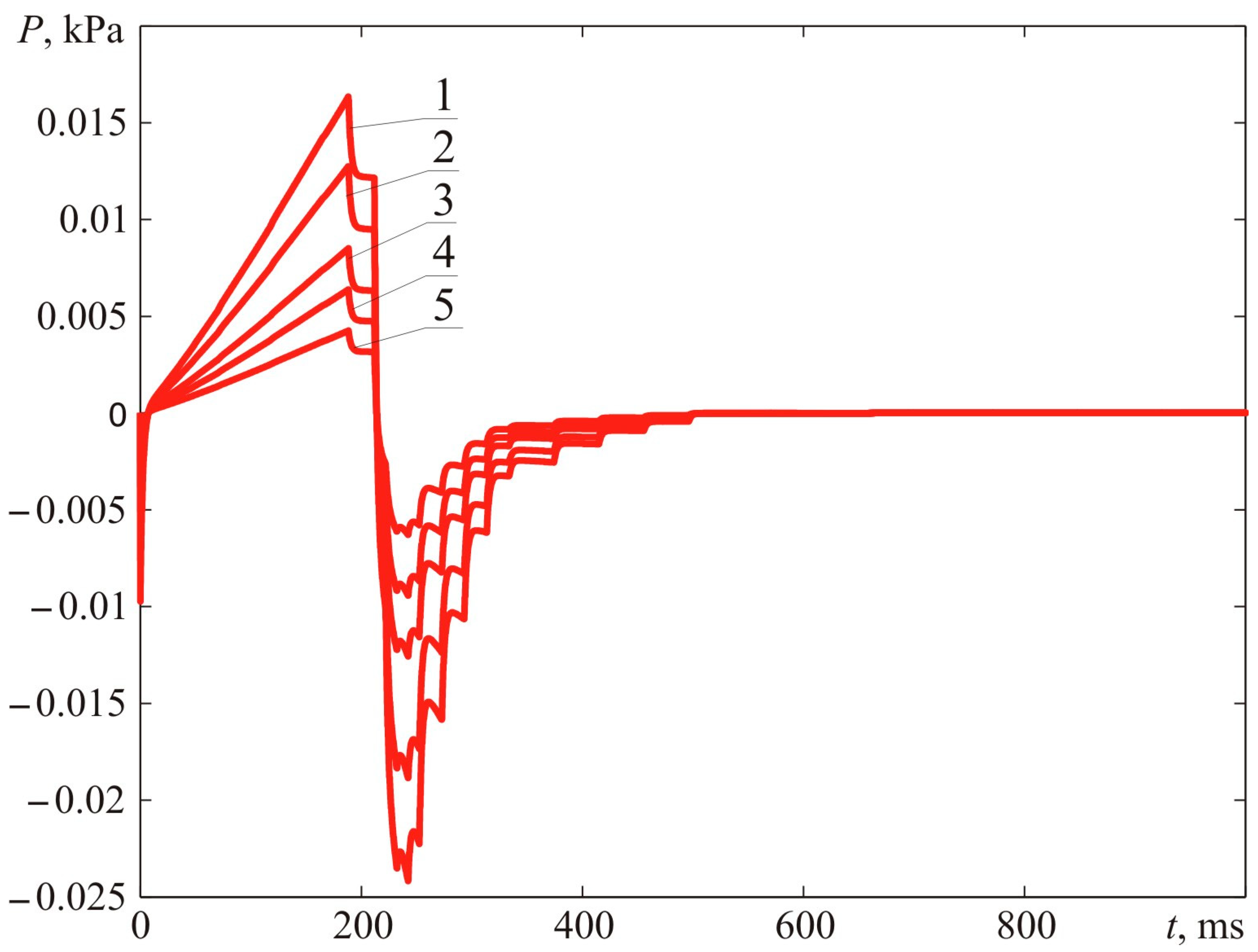
Figure 12 demonstrates the dynamic parameters of blast pressure at distances of 0.78, 1.00, 1.50, 2.00, and 3.00 m from the ignition spot. The distance R = 0.78 m corresponds to the maximum dimension of the fireball.
Figure 13 reveals the calculations for the blast pressure spectrum. The narrow-band spectrum demonstrated in
Figure 13 suggests that the main acoustic (vibrational) load is allocated within the low-frequency sector. Thus, if the dimensions of the gas-contaminated area grow at the same visible flame propagation rate, the acoustic (vibrational) load shifts towards the low-frequency sector. At a certain point, the human ear stops perceiving the leading share of the vibrational load, which rests within the infra-sound frequency range. As a result, the actual damage caused by accidents often does not match the reports of eyewitnesses who claim they heard no explosion but just a buzz or even some kind of hiss.
At the same time, the eyewitnesses perceive the accidental explosion as a flash fire, not accompanied by excessive pressure but by a wind gust or a short-term wind load [
10,
11,
12,
13]. However, the actual situation is different. For example, a 10 kPa compressive wave (one-ton force over a square meter) is accompanied by a wind gust with a wind velocity of just 34 m/s.
Below is an analysis of the experimental data pertinent to an explosion of a propane–air mixture with turbulizers designed to accelerate the explosive combustion process (Experiment 1).
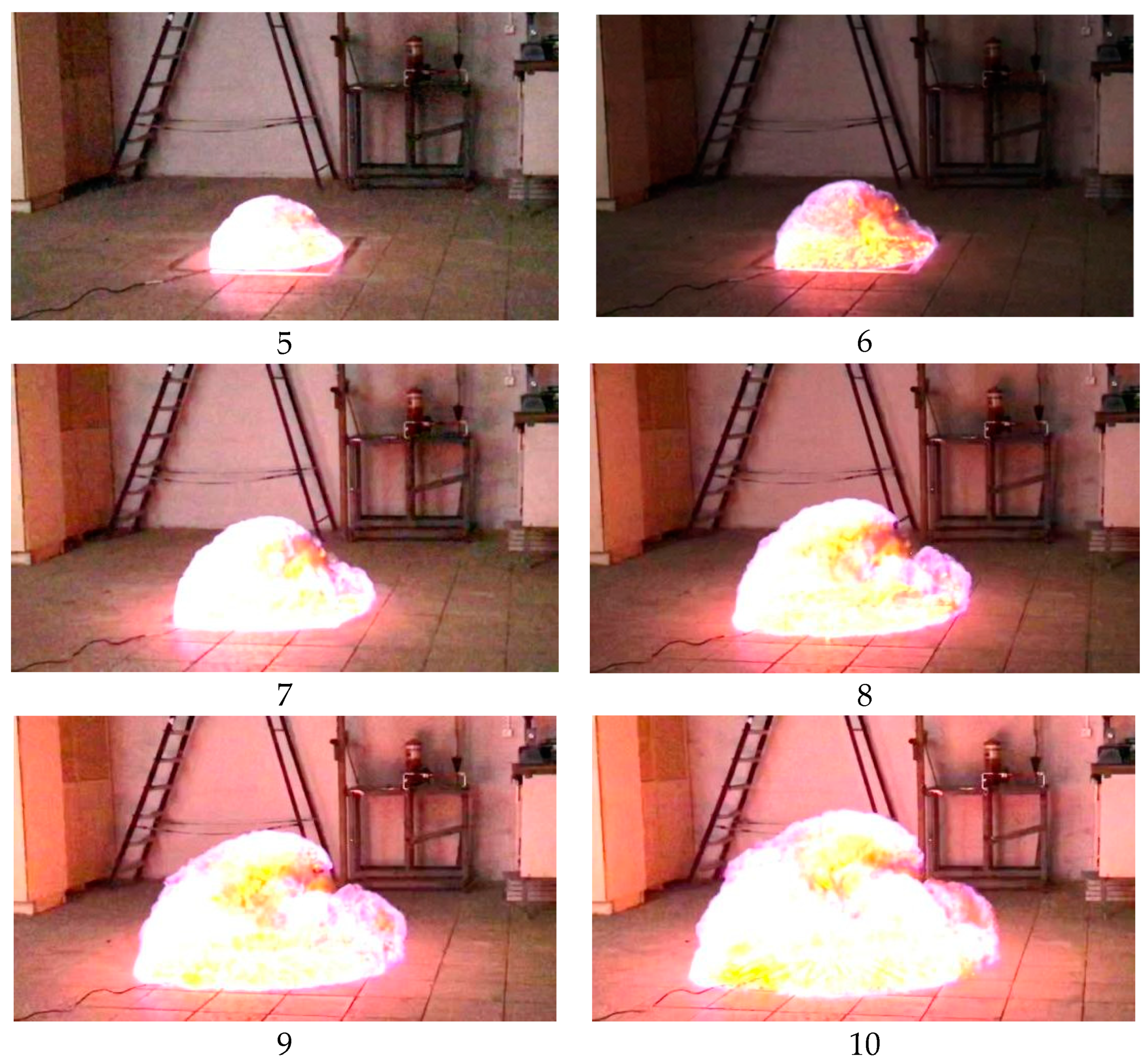
Figure 14 provides photos of a deflagration explosion every 25 ms (every six frames) obtained for Experiment 1.
Figure 15 provides experimental points describing the front flame location versus time characteristic and the interpolation curve.
Figure 16 provides a derivative of the interpolatory relation, which describes the visible flame propagation rate. Apart from that,
Figure 16 contains points that represent numerical values of the flame propagation rate obtained through a formal computation of the time derivative. The latter, in its turn, was obtained based on experimental values of the flame front location indicated with points in
Figure 15.
There were calculations of supposed time relationships of blast pressure generated by the explosion.
Figure 17 demonstrates the dynamic parameters of blast pressure at 0.75, 1.00, 1.50, 2.00, and 3.00 m from the ignition spot. The distance of R = 0.75 m corresponds to the maximum dimension of the fireball.
7. Discussion of Experiment Results
The kinematic parameters of the flame front assumed in the calculations correspond to the data obtained from the experiment (see
Figure 15 and
Figure 16).
Here we should again point out the specific aspects of emerging vibrational or acoustic loads caused by deflagration explosions and how humans perceive them [
5,
6]. The importance of this remark is stipulated by the fact that for real-life accidents, the witness reports (based on perceived blast loads) constitute the primary source of information about the explosion.
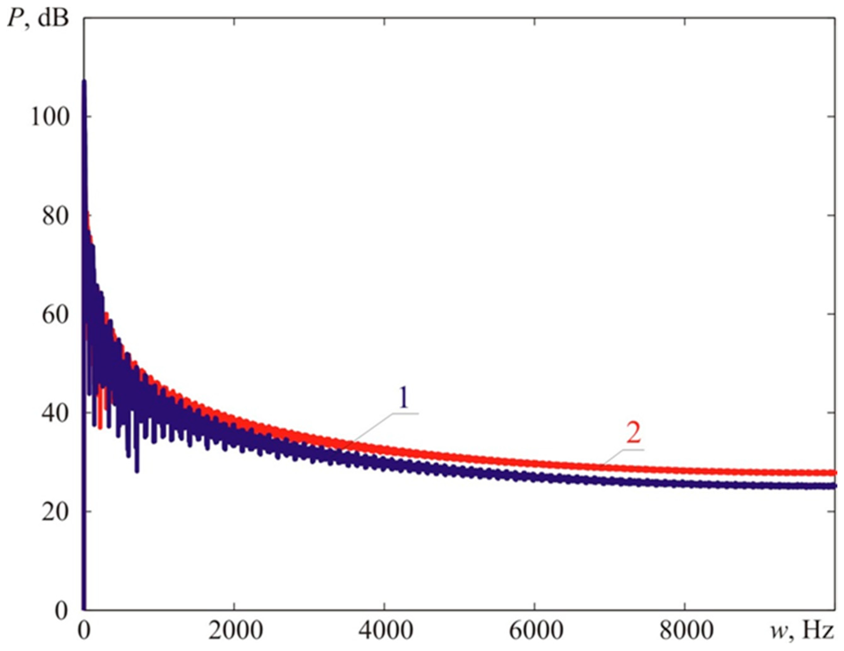
Figure 18 provides a comparison of narrow-band (the bandwidth of 1 Hz) spectra of blast loads registered at the distances that correspond to the maximum dimensions of fireballs during Experiment 1 and Experiment 2, as described above.
The calculations suggest that the vibrational characteristics of blast loads obtained during Experiment 1 using turbulizers are higher than those in Experiment 2 (without turbulizers). The calculations demonstrated [
19,
20] that the overall intensity of the vibrational load for Experiment 1 is 131.0 dB, whereas, for Experiment 2, it comprises 129.3 dB. However, the maximum value of the blast pressure in Experiment 1 is higher than in Experiment 2 (see
Figure 12 and
Figure 17). The maximum blast pressure in Experiment 1 is 0.0522 kPa, whereas in Experiment 2, it reaches 0.0163 kPa, which is 3.2 times higher [
21].
On the other hand, the acoustic intensity of the blast load for Experiment 1 (oscillation frequencies higher than 22.5 Hz) constitutes 119.6 dB, which is lower by 2.5 dB compared to Experiment 2, where the acoustic intensity of the blast load comprises 121.9 dB. This can be vividly seen in
Figure 18, where the high-frequency part of the Load 1 spectrum is lower than the respective part of the Load 2 spectrum. Hence, people will perceive a weak explosion without turbulizers (Experiment 2) as more intensive compared to the one where turbulizers were present (Experiment 1) [
22,
23,
24,
25]. It should also be noted that 2.5 dB is quite a noticeable value for a human.
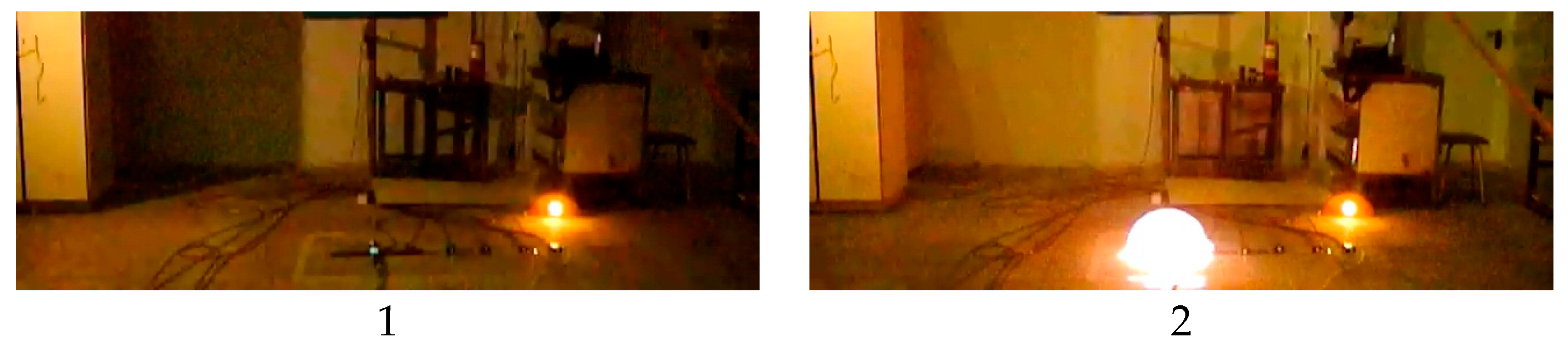
Let us review the results of a test explosion of 40 L of acetylene placed inside the cube. The photo and a general schematic are given in
Figure 7 and
Figure 8. A stoichiometric acetylene–air mixture was created inside the cube [
26,
27,
28,
29]. Shifting the upper lid sideways and rapidly lifting the cube can simulate a free (atmospheric) explosive cloud.
The ignition source was on the floor (ground surface) and was a gas cooker lighter. Hereinafter, we will refer to the experiment as Experiment 3.
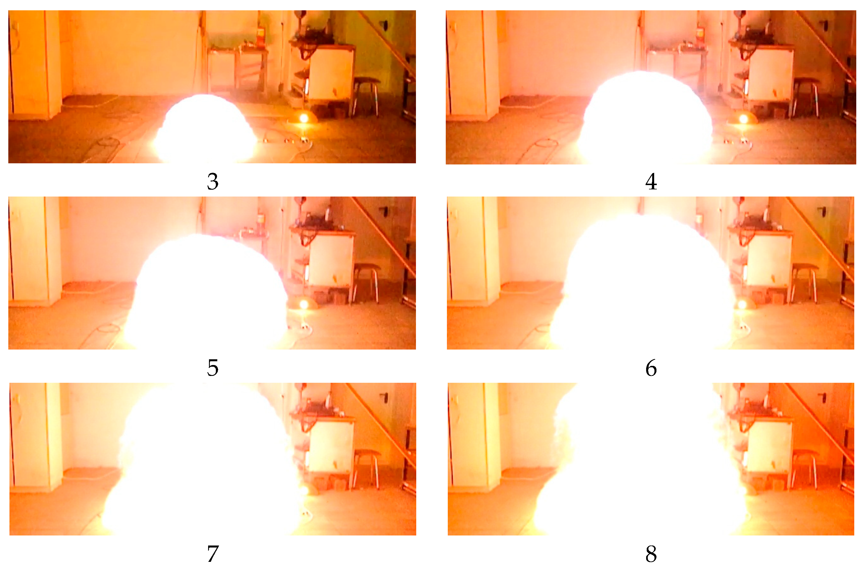
Figure 19 contains photos of an explosion within Experiment 3 taken from the 400-fps video.
Figure 19 shows every 5th frame, and the time interval between the photos is 12.5 ms.
Figure 20 provides temperature–time laws in the points located on the floor 0.2 m away from each other (see
Figure 20, Picture 1). The temperature sensors located on the floor can be well spotted in the photos provided in
Figure 20. Their location is more vividly seen in the photos of the moment when explosive combustion is initiated, i.e., in the first photo.
Point 1 is located 0.2 m away from the ignition source; point 2—at a distance of 0.4 m; point 3—at a distance of 0.6 m; point 5—at a distance of 0.8 m; point 5—at a distance of 0.4 m from the ignition source.
Figure 20 delivers several important messages which should be considered when computing excessive pressure generated by a deflagration explosion. First, the temperature of explosion (combustion) products in points 1, 2, and 3 located 0.2, 0.4, and 0.6 m, respectively, away from the ignition source (which constitutes about 75% of fireball dimensions), reaches 1890 °K, which is 24% lower than the combustion temperature of a stoichiometric mixture. Therefore, incomplete combustion occurs, or the mixture is diluted by ambient air during the experiment (explosion), and its concentration decreases (the mixture becomes leaner). Second, the temperature of explosion products in point 4, located 0.8 m away from the ignition source, i.e., at the fireball boundary, dropped significantly and constituted 1450 °K, which is only 75% of the temperature of combustion products in the central part of the fireball (in points 1, 2, and 3). However, in point 5, located 1 m away, the temperature was just about 500 °K. At the same time, the photos given in
Figure 19 suggest that the fireball radius is about 1 m, i.e., all temperature sensors fall within the impact zone of the fireball.
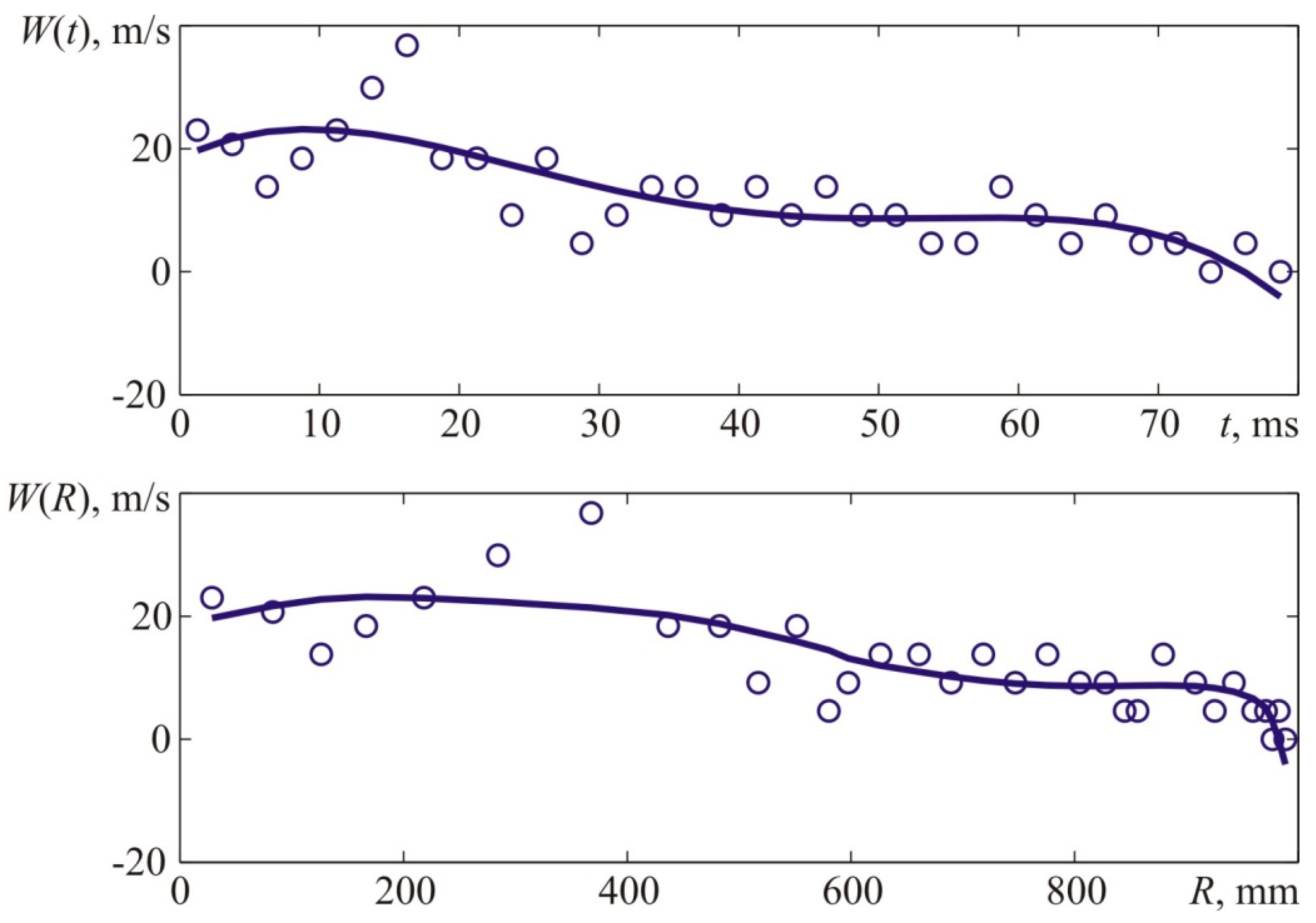
Similarly to previous experiments, kinematic parameters of the flame front were determined for test 3.
Figure 21 provides experimental points describing the front flame location versus time characteristic and the interpolation curve. Interpolations were performed with fifth-order polynomials, and
Figure 22 provides a derivative of the interpolatory relation representing the visible flame propagation rate. Apart from that,
Figure 22 contains points that represent numerical values of the flame propagation rate obtained through a formal computation of the time derivative. The latter, in its turn, was obtained based on experimental values of the flame front location indicated with points in
Figure 21.
It is worth reminding that the stoichiometric acetylene–air mixture’s normal flame front propagation rate (7.75% vol.) is 1.61 m/s, whereas the expansion rate of combustion products is 8.9. Thus, the visible flame propagation rate (for laminar flame spreading) is 14.3 m/s.
The maximum flame propagation rate value obtained during the experiment and determined with the interpolation curve (
Figure 22) constituted 23.14 m/s.
Let us take a look at and analyze the data acquired during an explosion of an acetylene–air mixture without the use of turbulizers (accelerators of the explosive combustion process) [
30,
31,
32,
33,
34] and with the ignition source located 0.7 m above the floor (Experiment 4). The explosion was filmed at the frame rate of 240 frames per second.
Figure 23 provides photos of the explosion during Experiment 4 (every 3rd frame). The time interval between the photos is 12.5 ms.
Similarly to previous experiments, kinematic parameters of the flame front were determined for test 4.
Figure 24 provides experimental points describing the front flame location versus time characteristic and the interpolation curve. Interpolations were performed with fifth-order polynomials, and
Figure 25 provides a derivative of the interpolatory relation representing the visible flame propagation rate.
The maximum flame propagation rate value obtained during the experiment and determined with the interpolation curve (
Figure 25) constituted 20.8 m/s.
The blast pressure sensor was located on the floor 1 m from the explosion site. The elevation of the ignition source was 0.7 m, and the distance from the lower end of the bar (by the floor) to the sensor location point was 0.7 m.
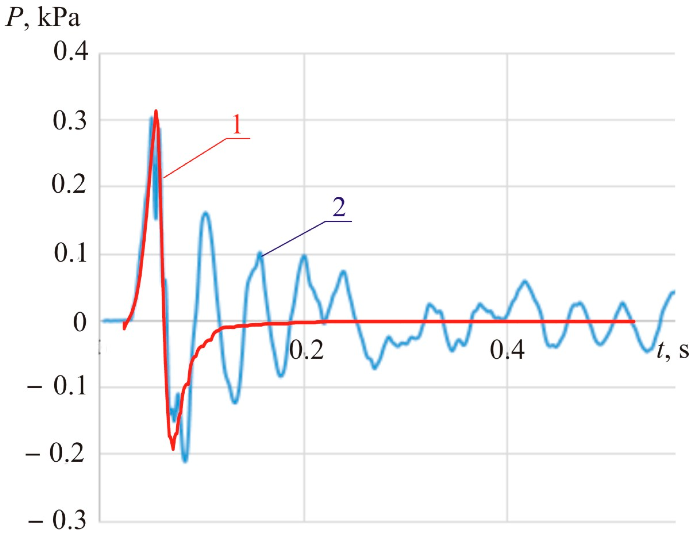
There were calculations of a supposed time relationship of blast pressure generated by the explosion.
Figure 26 demonstrates the dynamic parameters of blast pressure at 1.00 m from the ignition spot. The maximum fireball dimension constituted R = 0.896 m.
The kinematic parameters of the flame front assumed in the calculations correspond to the data obtained from the experiment (see
Figure 24 and
Figure 25). The maximum blast pressure at a distance assumed in the calculation is Δ
PMAX = 0.51 kPa. The minimum blast pressure is ΔP
MIN = −0.31 kPa. The calculations were conducted according to the algorithms described in [
5,
6].
Figure 27 demonstrates experimental values of blast pressure 1 m from the explosion site.
The visual comparison between calculation results and the experimental data (
Figure 26 and
Figure 27) suggests that calculations provide higher (overestimated) values of blast pressure for the experimentally registered visible flame propagation rate.
It is attributed to the fact that the calculation model assumes blast process patterning based on the flame front kinematics that defines the medium motion and, correspondingly, the pressure outside the combustion area [
19,
20]. However, as pointed out earlier, temperature sensors demonstrate (see
Figure 20) that the explosive combustion process is incomplete (the temperature of combustion products does not reach the required value), or the fireball dimensions obtained from photos provide overestimated values. One of the reasons why the temperature of combustion products does not reach the required value may be that behind the flame front, there remain burning fragments of the combustion mixture. In the photos of the acetylene–air mixture explosion shown in
Figure 19 and
Figure 23, this process cannot be seen due to the high brightness of the combustion process. Thus, it is more convenient to refer to photos of the propane–air mixture explosion (see
Figure 9 and
Figure 14).
Considering that, as experiments have shown, there remain burning fragments of the combustion mixture behind the flame front, which affects, among other things, the temperature characteristics of the explosion products, an adjusting coefficient should be introduced to the calculation model [
32,
33,
34]. We have brought in the following adjusting coefficient
where
ε = 8.9 is the expansion rate of combustion products.
K = 0.7 is the coefficient factoring in the burning fragments of the combustion mixture behind the flame front. The temperature of the explosion products does not exceed 75–80% of the combustion product temperature for a stoichiometric mixture.
Figure 28 provides the calculated dynamic parameters of the explosion for Experiment 4 with the introduced adjustments. Calculations of blast pressure were performed for the distance of 1.00 m from the ignition spot. Considering the introduced adjustment, the calculated value of the maximum blast pressure at the distance of
R = 1 m constituted Δ
PMAX = 0.3169 kPa, whereas the minimum blast pressure comprised Δ
PMIN = −0.1923 kPa.
Figure 29 compares the calculated dynamics of blast pressure with the one obtained during Experiment 4.
The wave motions registered during experiments and accompanying the compression and negative waves following a deflagration explosion appear due to the presence of walls in the laboratory where the tests were held [
9,
21].
The 30 ms compression wave (see
Figure 28) lasts about 10 m. Therefore, in the case of an indoor explosion (with reflecting walls, floor, and ceiling), standing waves are picked up by the pressure sensor. The dissipation of standing waves, however, in a standard room (with no absorbing surfaces) takes a considerably long time. It requires a period that comprises 10 to 20 blast pressure periods (see
Figure 29).
Figure 29 suggests that indoors, the wave attenuation requires at least 500 ms, which is about 17 times more than the duration of the compression phase of a deflagration explosion.
8. Conclusions
Physically, the simulation of outdoor (atmospheric) accidental deflagration explosions is troublesome. It is due to the practical difficulties of creating a stable explosive cloud of the combustible mixture as it is affected by moving ambient air. However, mathematical models of explosion processes require experimental validation.
The contributors to the present article have managed to experimentally justify the methodology, which allows the creation of an unconfined cloud of the combustible mixture of a given blend composition and shape. There have been demonstrated examples of modeling studies of accidental atmospheric explosions and providing analysis of the acquired experimental results. It has been demonstrated that with the help of a testing rig located inside a large room, it is possible to create a combustible mixture of stoichiometric or other concentrations in a shape of a sphere (for lighter-than-air flammable gases) or a hemisphere supported by ground (for heavy gases, e.g., propane).
Further, analysis of the experimental data obtained allowed us to clarify several aspects of the explosive combustion of atmospheric gas–air clouds. Notably, the pattern of fireball temperature reduction as a function of distance has been pointed out and determined the visible flame propagation rate.
The article calculates the supposed time relationships of blast pressure generated using the explosion. The calculations were performed by the methodology describing the pressure pattern outside a pulsating sphere, simulating an expanding ball of combustion products following a deflagration explosion [
6,
7]. It has been demonstrated that it is the most reasonable to base computational experiments on linearized (acoustic) equations of continuum motion, as the visible flame propagation rate emerging during explosive combustion is small (compared to the speed of sound).
As experiments have shown, burning fragments of the combustion mixture remain behind the flame front, which affects, among other things, the temperature characteristics of the explosion products. That is why the calculation model was complemented with an adjusting coefficient factoring in that the temperature of the explosion products does not exceed 75–80% of the combustion product temperature for a stoichiometric mixture. Concerning the introduced adjustment, a satisfactory agreement has been achieved between the calculation results and the obtained experimental data.


 ,
, 


