Article

Emission Factors for the Burning of Decking Slabs Made of Wood and Thermoplastic with a Cone Calorimeter

by
Bruno Martinent
*,
Karina Meerpoel-Pietri
,
Svetlana Petlitckaia
,
Toussaint Barboni
,
Virginie Tihay-Felicelli
and
Paul-Antoine Santoni
SPE-UMR 6134 CNRS, University of Corsica, Campus Grimaldi, BP 52, 20250 Corte, France
*
Author to whom correspondence should be addressed.
Fire 2023, 6(4), 162; https://doi.org/10.3390/fire6040162
Submission received: 8 February 2023 / Revised: 3 April 2023 / Accepted: 12 April 2023 / Published: 17 April 2023
(This article belongs to the Special Issue Atmosphere Fire Interactions)

Abstract

:
Smoke is an important component of wildfires. Specifying the combustion process of different materials allows scientists to better prevent and adopt public health measures. This experimental study contributes to a better characterisation of the smoke emitted by two types of decking, wood and thermoplastic, commonly used in terraces. Emission factors were characterised using a cone calorimeter for different incident fluxes ranging from 10 to 50 kW/m2. The study showed that compared to wooden (pine) decking, thermoplastic (polypropylene) decking produces more gases and aerosols, less VOCs, but with a chemical composition that is more carcinogenic.

1. Introduction

Wildfires are a major problem: 700,000 hectares burn every year in Europe [1] and almost 350 million hectares worldwide. France, with its 15 million hectares of forest, is particularly vulnerable to forest fires, especially in the Mediterranean region, where the Corsican forest covers an area of 550,000 hectares [2]. These fires can be of natural or anthropogenic origin. They cause human tragedies, significant economic losses and damage to ecosystems, especially in the wildland–urban interface (WUI). WUI management for wildfire mitigation has become an increasingly critical issue in recent years in many Mediterranean regions of the world. WUI fires have caused significant destruction of infrastructure in many parts of the world [3]. For example, in 2020, according to the National Interagency Coordination Center [4], the USA recorded 58,950 wildfires that burned 10,122,336 acres and destroyed 17,904 structures.
The recent increase in large forest fires along the WUI has had huge social and environmental impacts around the world. If trends in land use planning or climate change continue, this problem could become even more serious in the future as urbanisation meets natural areas. The WUI threatens wilderness areas, while the high intensity of large wildland fires contributes to their destructive power when they reach the WUI [5]. Changes in the geography of cities and the expansion of forests mean that these wildland–urban interfaces are increasingly present. The development of structures adjacent to wildland and forest areas increases the risk of fire in interface areas by increasing the number of ignition sources and the vulnerability of infrastructure. These situations force operational resources to prioritise the protection of people and property to the detriment of firefighting [6]. In particular, during large fires, firefighting operations are penalised on the active parts of the flame fronts, leading to an increase in the areas covered. Reducing the vulnerability of the interface between the natural environment and buildings is therefore an important issue in the fight against vegetation fires. We also know that the effects of large forest fires in southern Europe may be exacerbated in the future by climate change [7].
These fires emit large quantities of smoke, which is dangerous because of its toxicity, but also because of its opacity, which impairs visibility [8]. They affect air quality on a global scale. In Indonesia, Malaysia, Central America, Russia, Mexico and the United States, multiple deaths from air pollution have been observed [9]. Toxicity may be acute or chronic. The different gases produced by smoke from fires can be asphyxiant, irritant or toxic [10]. Forest fire smoke is a complex mixture of gases, volatile organic compounds (VOCs) and aerosols [11,12,13,14,15,16]. These primary pollutants undergo physicochemical transformations in the atmosphere, giving rise to secondary pollutants. Many studies have analysed the composition of smoke emitted by wildfires under fire conditions during prescribed burns or in the laboratory [11,16,17,18,19,20,21,22]. Firefighters and people living near the fire are at risk from the smoke. According to the WHO, aerosols are responsible for 1.4% of deaths worldwide [23] and are a factor in reducing life expectancy. In Europe, for example, a reduction of 8.2 months has been observed.
In the WUI, among the various structural elements, deck assemblies are identified as vulnerable materials [24]. Indeed, these elements are generally made of combustible materials such as wood or plastic. Not only the fire behaviour is necessary to assess vulnerability in the WUI, but smoke production is also important to determine the exposure of the nearby population or of firefighters. The aim of this study is to characterise the emission of pollutants in each phase of combustion (pyrolysis, flaming, glowing). Two types of decking slabs were used: one in wood and one in thermoplastic. Different heat fluxes ranging from 10 to 50 kW/m2 were applied to the top of the fuel samples using a cone calorimeter [25]. Several studies using a cone calorimeter have already been carried out with wood [26] or plastic [27,28], but to our knowledge, no studies have been undertaken with combined measurements of gas, volatile organic compounds and aerosol. This study provides refined data on emission factors that can be used as input data in physical models according to the combustion phases that occur in the different fire areas. This paper first introduces the studied fuels and the experimental methods used to study the combustion of those fuels. We discuss the mass loss rate (MLR), heat release rate (HRR), smoke production rate (SPR), smoke extinction area (SEA) and all emission factors (EF). Finally, a carbon balance was carried out to assess the consistency of our analyses.

2. Materials and Methods

2.1. Fuel Sample

Experiments were carried out with two types of decking. The first was made of wood (pine) and the second was made of thermoplastic (polypropylene). The materials were bought from DIY stores. To remove moisture from the samples, the boards were first dried in an oven at 60 °C for 48 h. The results of the elemental analysis of the wood and thermoplastic panels are presented in Table 1 (NF EN 15407). The remaining percentages are mostly ash at 815 °C for the wood samples and calcium oxide from calcium carbonate degradation, which was used as filler, for the thermoplastic samples. Traces of chlorine, sulphur and non-volatile minerals were also revealed.
Both decking slabs measure 40 × 40 cm2. The wood slabs are autoclaved and treated against biological attack by insects and fungi. They are classified as type 3 according to NF EN 335, which means that they can be exposed to alternating periods of dampness and dryness. The thermoplastic slabs are made of polypropylene and calcium carbonate added as a filler. Due to their size, the slabs could not be placed directly under the cone heater, so they were cut. In order to respect their original geometry as much as possible, we designed samples with the following dimensions: 60 × 60 × 11.5 mm³ for the wooden slabs, giving an average mass of 21.2 (±2.0) g and an exposed surface area of 3600 mm2. The thermoplastic slabs were cut to the following dimensions: 72.5 × 72.5 × 12.6 mm³, giving an average mass of 48.8 (±1.9) g. As the thermoplastic slabs have holes, the exposed surface area is the same as for the wooden slabs, i.e., 3600 mm2.

2.2. Experimental Methods

The samples were burned using a cone calorimeter (Figure 1) coupled to an Antaris IGS FTIR Spectrometer (Thermo Fisher Scientific, Waltham, MA, USA). The cone calorimeter is composed of a cone heater, a shutter, a load cell and an exhaust system with gas analysers. Samples were exposed to a radiant heat flux ranging from 10 to 50 kW/m2. For each radiant flux, five measurements were made for wood and three for thermoplastic. This range of values was chosen because it corresponds to the levels of heat flux measured in shrubland fires ahead of a fire front [29]. The fuel was preheated by the cone heater, which led to its gasification. After the ignition, the sample burning occurred in two stages for wood. Flaming combustion was observed first. Its duration depends on the thickness of the sample and available mass. Then, once the flames extinguished, a short degradation continued for the thermoplastic, while for wood, the embers remained and glowing combustion followed. By using an open basket, the combustion was over-ventilated. After the complete consumption of embers, extinction occurred and only ashes remained. Further cone calorimeter details are provided in a previous publication [30].
The heat release rate is given by the oxygen molar flow rate:
H R R = E n ˙ O 2 0 n ˙ O 2 W O 2 ,
where E is equal to 13.00 MJ/kg for wood and 12.39 MJ/kg for thermoplastic and corresponds to the heat release per unit mass of O2 consumed, n ˙ O 2 0 a nd n ˙ O 2 represent, respectively, the molar flow rates of O2 in the incoming air and in the exhaust duct and W O 2 is the molecular weight of oxygen. More details on HRR measurement are given in a previous study [30].

2.3. Chemical Analysis of Smoke and Emission Factors

Smoke from forest fires includes important amounts of gases, aerosols (PM) and other chemical compounds like volatile organic compounds (VOCs). The generation of combustion products was quantified in terms of emission factors, EFi (g/kg). Emission factors are defined as the mass of chemical species i produced per unit dry mass of fuel burned [31].
E F i = m i m b , d r y
where m i (kg) is the mass of compound i released by the burning and m b , d r y (kg) is the dry mass burned during the experiments.
The exhaust gases of combustion were sampled from the exhaust ducts of the cone calorimeter and passed through four different measurement systems. The first measurement system consists of an Antaris Industrial Gas System (IGS) FTIR-based analyser from Thermo Fisher Scientific. The FTIR spectrometer obtained the molar fractions of CO2, CO, CH4, NO, NO2, NH3, C2H6, C2H4, C2H2, C3H8, C3H6, C4H6, C6H6, HCHO, CH3CHO, SO2 and H2O. A filter removing the aerosols (0.45 µm pores) was placed before the gas cell and the sampling line and was heated at 180 °C to avoid condensation. The spectrometer was equipped with an MCT-A detector and a gas cell measurement with a volume of 0.2 L and an optical path length of 2 m. IR spectra were recorded in the spectral range of 4500–550 cm−1 with a 0.5 cm−1 resolution. The flow rate of the sampling pump was adjusted to 3.5 L/min. The identification of the compounds by FTIR was carried out from a bank in which the products resulting from the combustion are listed. Calibration verification is performed once a year by a maintenance engineer from Thermo Fisher. The second measurement system consists of non-dispersive infrared (NDIR) spectroscopy. This apparatus was used to quantify continuously CO and CO2. Each day of analysis, NDIR analysers were calibrated with two points of measurement. The first point corresponds to a gas without CO and CO2. For this, almost pure N2 (99.995% i.e., 4.5) was used. For the second point, a mixture containing 2500 ppm of CO and 8% CO2 was used. These measurements performed a double check on the CO and CO2 data recorded by the FTIR. The third system is an automatic thermal desorption gas chromatography–mass spectrometry apparatus (DTA/GC/MS) for VOC identification and quantification. A sample pump with a flow rate of 1.4 L/min was used to collect VOCs with Tenax tubes (Supelco®, Saint-Quentin-Fallavier, France). Upstream of the pump, glass fibre filters, type A/E (DOP efficiency is 99.98% at 0.3 µm), were used to prevent aerosol from penetrating the Tenax TA tube. Since the sampling took place in the smoke extraction pipe, where the flow rate was 24 L/s, a multiplicative factor of 720 was used to calculate the emission factors. At least three tests were carried out to ensure reproducibility for each slab. The Tenax TA sorbent tubes used for the analyses had the following dimensions: 115 mm × 6 mm outer diameter (o.d.) × 4 mm inner diameter (i.d.), in order to capture the organic compounds (C5-C30). The analyses were performed by thermal desorption using the DTA-GC/MS. It should be noted that sorbent tubes have previously been used in other studies for sampling VOCs and SVOCs [32,33] before GC/MS analysis.
The analyses were carried out immediately after filling the Tenax tubes using a DTA TurboMatrix from PerkinElmer. For the thermal desorption of VOCs, H2 flow was set at 30 mL/min with a column head pressure at 25 psi. The sorbent tube was brought to 280 °C over 10 min and a carrier gas flushed the sample towards a cold trap at 5 °C. In a second step, the cold trap (22 cm, 0.53 mm i.d.; Supelco) was programmed to increase the temperature from 5° to 280 °C at 40° C/s and then hold isothermally at 280 °C for 3 min. The compounds were then desorbed onto the chromatograph under H2 as carrier gas via a heated transfer line maintained at 280 °C. The ionization energy for mass detection was set to 70 eV and electron ionisation mass spectra were acquired over the mass range 35–350 Da. The chromatograph and mass spectrometer was a Perkin Elmer Clarus 500® apparatus (Waltham, MA, USA). The chromatograph was equipped with a non-polar column (Rtx®-1 fused silica column, dimethylsiloxane, Resteck, Lisses, France) with a length of 60 m and i.d. of 0.22 mm. This column was coupled with the mass detector. Detection was carried out by a quadripolar analyser made up of an assembly of four parallel electrodes of cylindrical shape. The oven temperature of the chromatograph was programmed from 50° to 260 °C at 2 °C min−1 and then held isothermally at 260 °C for 10 min. The methodology used to identify individual components was based on a comparison of their GC retention indices (RI) on non-polar columns with those of authentic compounds or literature data [32,34]. The RIs on nonpolar columns were determined relative to the retention time of a series of n-alkanes with linear interpolation. The results were computer-matched with commercial mass spectrum libraries [34] and spectra were compared with those in our own library of authentic compounds. The majority of these compounds were commercial standard components. The relative amounts of the individual components were calculated on the basis of their GC peak areas, obtained on a second capillary Rtx-1 column, with flame ionisation detector (FID) response factor correction. Quantification was performed for equivalent benzene with GC/FID. The method of external calibration used was from a commercial standard (Restek, Lisses, France). Triplicate injections of standards were made for each set of concentrations (5 different concentrations) for the curves of external calibration standards. A total of 5 calibration points were made. The correlation coefficient (R2) for the linear regression of the curve of external calibration standards is 0.996, indicating a good correlation between the detector’s response and the concentration of injected products. The identification and quantification methods of the chemical compounds were described in a previous study [11]. Before each sampling, Tenax tubes were conditioned for 15 min at 280 °C. Each day, a “blank analysis” was performed after conditioning the tubes to avoid or observe contaminants.
Finally, the fourth measurements correspond to the use of a He-Ne laser in order to assess aerosol mass concentration. Smoke obscuration was measured in the exhaust duct with a He-Ne laser (0.5 mW nominal power) emitting at the red wavelength of 632.8 nm. The length of the optical path in the exhaust duct is 11.4 cm. The smoke production rate (SPR) was calculated according to the basic smoke equation:
S P R = k V ˙
where k is the light extinction coefficient given by Bouguer’s law and V ˙ is the standard flow rate in the exhaust duct. The specific extinction area, SEA, was calculated, which corresponds to the ratio of the smoke production rate to the mass loss rate (MLR):
S E A = S P R M L R
The mass of aerosol m a released during the burnings was calculated using the following equation:
m a = 0 T k σ a V ˙ d t
where σ a (m2/kg) is the mass specific extinction coefficient. The values obtained by [35] for σ a were used: σ a = 8290 m2/kg during the flaming stage and σ a = 3290 m2/kg during the preheating and smouldering stage. Aerosols were also collected on glass fibre filters (37 mm diameter) sampled in the cone calorimeter duct by using a sample pump in order to assess σ a for thermoplastic slabs.
Elemental carbon (EC) and organic carbon (OC) analyses of aerosols (Table 2) were done with a technique that combines evolutionary thermal optical analysis (TOA) and flame ionization detection (FID) by the Analytice® company, according to the NIOSH 5040 method.
The measurement of EC and OC contents as well as their ratio is a first step to perform a carbon mass balance, essential for better knowledge of the particle sources. EC refers to soot carbon, a purely primary compound, related to pure graphite. It is emitted during the flaming phase. OC comes either from thermal degradation or organic compounds from the smoke that adsorbs on the particles already formed during combustion.
A total carbon mass balance (CMB) was used to check the quantities of emitted gases. Indeed, when quantifying emitted compounds, one must check that the analysed carbon content does not exceed that found in the fuel by ultimate analysis. Hence, the amount of carbon C M B i of each assayed compound i was calculated in grams of carbon per kilogram of plant according to the following equation:
C M B i = E F i × W c W i × n c ,
where Wc and Wi are the molecular weights of carbon and compound i, respectively, and nC is the number of carbon atoms present in compound i.

3. Results

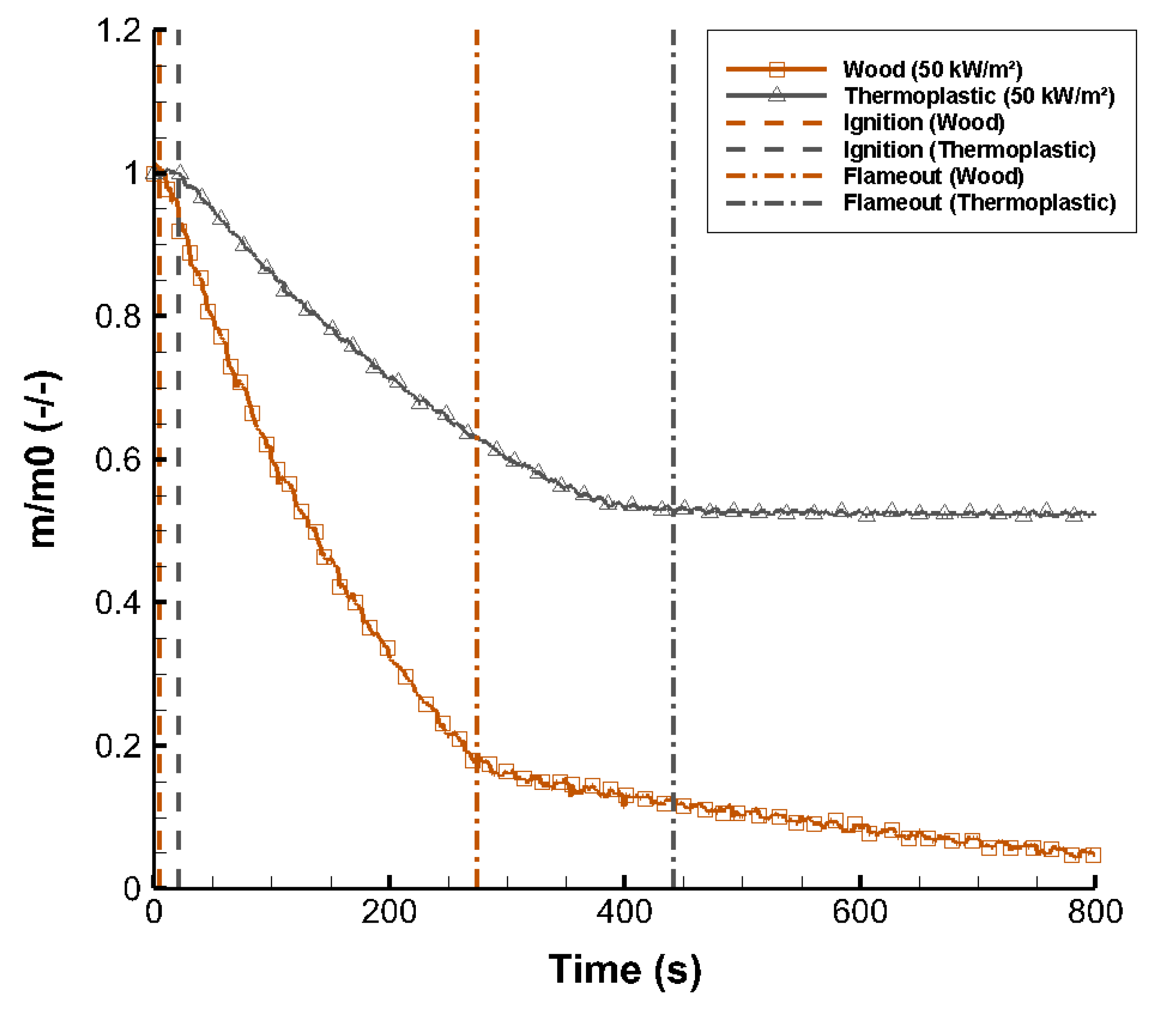
3.1. Mass Loss Rate (MLR)

Figure 2 shows the non-dimensional mass loss, m / m 0 (where m and m 0 are the mass over time and the initial mass of the samples, respectively), as a function of time for wood and thermoplastic decking slabs for one experiment representative of the set of tests at an exposed heat flux of 50 kW/m2. A low mass loss is first observed prior to ignition, corresponding to a low emission of decomposition gases, water vapor and aerosols, and representing a loss of 5 ± 3% of the initial mass for the wood sample. For the thermoplastic, this first phase represents a mass loss of less than 1%. After ignition, the mass decreases significantly. For wood, the mass loss continues after flameout. In fact, 15 ± 5% of the initial mass is consumed during the glowing phase, as the wood produces char, which continues to burn after extinction. For thermoplastic, the mass loss occurs mainly during the flaming combustion and there is no smouldering phase after the flameout.
At the end of the tests, 2.67 (±1.47)% and 52.7 (±0.7)% of the initial mass for the wood and thermoplastic samples remains, respectively. For wood, the residue corresponds to ashes (Figure 3a). For the thermoplastic samples, the residue is white and friable and corresponds to the calcium carbonate used as filler (Figure 3b). This result reveals that all of the fuel mass corresponding to the thermoplastic has been consumed.

3.2. Heat Release Rate and Smoke Production Rate

3.2.1. Heat Release Rate

To better understand pollutant emissions, it is useful to measure the Heat Release Rate (HRR) emitted during the combustion phases. This allows the combustion dynamics to be understood. Figure 4 shows the HRR curves for wood and thermoplastic samples as a function of time for an imposed heat flux of 50 kW/m2 for one experiment representative of the set of tests. As already observed with the mass loss curves, the HRR curves show that the ignition time is longer for the thermoplastic than for the wood samples. After ignition, the HRR increases until it reaches a maximum for both samples (620 kW/m2 for wood and 700 kW/m2 for thermoplastic). After the peak, two behaviours are observed depending on the decking slab. For both slabs, the HRR decreases immediately after the peak HRR (PHRR). For the thermoplastic slabs, we observe a slow and continuous decrease after the PHRR until the flameout, and then the HRR drops to zero. For the wood slabs, after the flameout, the HRR continues to decrease slowly, corresponding to the glowing combustion of the char.
The combustion dynamics of both slabs were also investigated for imposed heat fluxes ranging from 10 to 50 kW/m2. Figure 5a,b show the curves of HRR versus time for the wood and thermoplastic slabs for the range of imposed heat fluxes investigated, i.e., 10, 15, 20, 25, 30, 35 and 50 kW/m2. Table 2 shows the PHRR, the time to ignition, tign, and the duration of the flame phase, tflam, for both samples. For the thermoplastic slabs (Figure 5b), the PHRR varies between 430 and 701 kW/m2 and increases with the heat flux density. The values obtained for the PHRRs are lower than those found by [36] for pure polypropylene samples (1166 kW/m2), but close to those found for polypropylene composites (448–615 kW/m2). In another study for polyethylene [37], the PHRR averaged 641.09 kW/m2 for an imposed heat flux of 50 kW/m2, which is close to the 701.1 kW/m2 found. For wood samples, the PHRR is between 226 and 639 kW/m2. These values are in line with those found for wood in the literature [38]. As for thermoplastic slabs, the PHRR values obtained for wood are constant up to an exposure value of 15 kW/m2, and then the PHRR increases linearly with the heat flux. As with thermoplastic slabs, the PHRR values obtained for wood increase with the heat flux density for heat flux densities greater than 15 kW/m2. It can be seen that the PHRR does not follow this trend for the lower heat flux value of 10 kW/m2. The reason for this is the long ignition time of about 450 s (Table 3). This could lead to an increase in the pyrolysis thickness through the sample and the release of a higher quantity of gases once the flaming condition is reached. It should be noted that the heat flux of 10 kW/m2 is close to the critical heat flux of ignition, which is 9 kW/m2. In this case, the behaviour is marginal.
For both types of slabs, the ignition time decreases as the radiant heat flux increases (Table 3). For a given heat flux, the time to ignition is always longer for the thermoplastic slabs than for the wood samples. However, as the applied heat flux increases, the difference between the ignition times of the two samples decreases. In fact, it is on the order of 71 s on average for heat fluxes less than or equal to 20 kW/m2. Then, for heat fluxes between 25 and 35 kW/m2, the difference between the ignition times of both slabs decreases to an average of about 34 s. Finally, for a heat flux of 50 kW/m2, it reaches 13 s. A previous study [37] found an average ignition time of 48.3 s for PE, which is higher than the 19 s found for thermoplastic. For 50 kW/m2, longer ignition times of 10 to 28 s have been reported [26] for different types of wood: spruce, oak, poplar and beech.
For both types of panels, the residence time of the flame decreases as the applied radiant heat flux increases (Table 3). The higher the heat flux, the higher the degassing rate and the shorter the combustion time. The lower values of residence time observed for the wood panels exposed to a heat flux density lower than 15 kw/m2 are due to the mass lost during the preheating phase. As the slabs ignite later at the lowest heat flux, a non-negligible mass of combustible gases is lost before ignition. This mass is therefore not available for combustion after ignition.

3.2.2. Smoke Production Rate

The Smoke Production Rate (SPR) quantifies the amount of aerosol emitted and its production phase. Wood and thermoplastic are two very different materials in terms of their structure, so it is interesting to compare them.
Figure 6 presents the SPR for wood and thermoplastic samples for an imposed heat flux of 20 kW/m2, corresponding to different times to ignition (on average, tign = 48 s for wood and tign = 108 s for thermoplastic). The experiments performed with an imposed heat flux of 20 kW/m2 are good examples to understand each peak of the SPR. Before ignition, a first peak is reached, which is the pre-ignition phase corresponding to the emission of aerosols without combustion (tars) for wood [35]. This peak is small compared to the second peak of SPR observed during the flaming phase. In a previous study concerning the burning of vegetation twigs [30], we observed the opposite. The reason might be due to the fact that vegetation twigs and wood burn differently, as shown in [39]. In Figure 6, we observe that the second peak of the SPR is higher than the first, which occurs in the pre-ignition phase, regardless of the fuel. The second peak of SPR after ignition is higher for thermoplastic, at 1.35 ± 0.15 × 10⁻² m2/s, than for wood, at 5.01 ± 0.5 × 10⁻³ m2/s, showing that thermoplastic is more smoke-producing than wood.
Combustion of the thermoplastic is very repeatable, allowing us to burn only three samples as opposed to five for wood. Figure 7a,b show the measured SPR versus time for the different imposed heat fluxes for the wood and thermoplastic samples. Each curve represents a single experiment for each flux. Adjustments were made to have the same time origin for all curves. During flaming, both the peak SPR and the area under the curve increase with heat flux, reflecting an increase in aerosol production quantified in Section 3.3.1. The peak SPR itself increases with flux from 0.005 to 0.019 m2/s for wood and from 0.006 to 0.03 m2/s for thermoplastic. As the heat flux increases, the first peak becomes indistinguishable as the duration of the ignition phase increases. In addition, the duration of the pre-ignition phase is shortened by faster ignition as the imposed heat flux increases. The peaks of SPR noted in the literature [27] are similar to those obtained in our study: 0.01–0.03 m2/s for wood flooring and 0.010–015 m2/s for PVC flooring.

3.2.3. Smoke Extinction Area

The specific extinction area, SEA, which is the ratio of the smoke production rate to the mass loss rate, is used here to compare the smoke production per unit burning mass for each phase, pre-ignition and flame. The mean and maximum SEAs for both phases are shown in Figure 8 for wood and Figure 9 for thermoplastic. For both materials, the maximum and mean SEA values follow the same trend. In addition, the SEA results are consistent with the SPR results. The higher the heat flux, the lower the time to ignition (Table 3), so for the pre-ignition phase, the duration of aerosol emission decreases as the heat flux increases. For the flame phase, the SEA increases slightly with the applied heat flux (Table 3). For thermoplastic, the maximum SEA in the pre-ignition part and the average SEA in the flame phase follow the same tendency as for wood (Figure 9a). However, in the pre-ignition part, the mean SEA varies too much to determine a variation due to the flux. For the flame phase (Figure 9b), the maximum SEA value does not vary with the heat flux. On average, the SEA of the thermoplastic is higher than that of the wood in both phases, as found in [40].

3.2.4. Heat Release Rate and Smoke Production Rate (HRR and SPR)

To analyse the simultaneous burning and smoke production of wood and thermoplastic slabs, the HRR and SPR of both samples are plotted in Figure 10 for the same imposed heat flux of 50 kW/m2. Upon ignition, both samples emit a large amount of heat and smoke, resulting in sudden peaks in HRR and SPR. Thermoplastic samples (Figure 10b) produce more smoke than wood during the flaming phase. Furthermore, the SPR for thermoplastics is almost constant for half the duration of the combustion phase, while a decrease in HRR is observed. This is not the case for wood, for which SPR and HRR follow the same decreasing trends over time during the combustion phase. For both samples, smoke production stops before the flame extinguishes. The wood samples (Figure 10a) continue to burn after the flame goes out without producing smoke.

3.3. Gas, Aerosols, VOC and SVOC Released

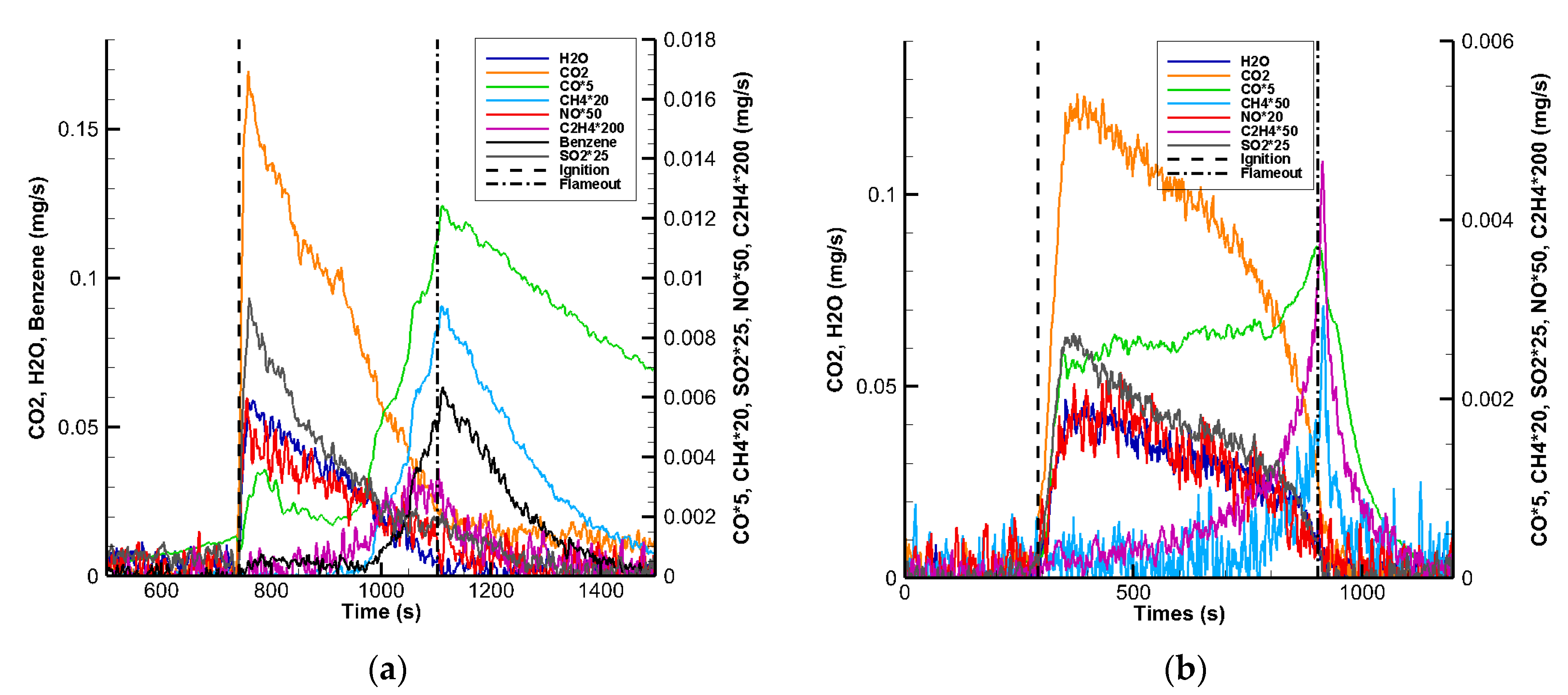
3.3.1. Production Rates of Gas Species According to the Phases of Degradation and Combustion

The main gases studied are H2O, CO2, CO, CH4, NO, NO2, C2H4 and SO2. Figure 11 presents the mass flow rates of these gases for an imposed heat flux of 10 kW/m2, allowing a visualizing of the pyrolysis phase in an optimal way. The curves were smoothed by averaging the values over 5 s, but they remain noisy. More powerful smoothing causes too much data loss.
For wood (Figure 11a), CO2 is mainly emitted during the flaming phase (82% of total CO2), like SO2 (61%) and H2O (73%). During the smouldering phase, the main gases emitted are CO (86%), CH4 (88%) and NO (50%). The compounds CO2, NO, SO2 and H2O follow the same trends. Their emissions increase after the ignition to reach a peak and then decrease until complete extinction. The emission of CO follows two steps: A first low-intensity peak occurs after the ignition; a second, more intense peak appears at the time of the flameout. For CH4, C2H4 and benzene, peak production occurs at the flameout and then decreases during the smouldering stage.
For thermoplastic (Figure 11b), CO2 is mainly emitted during the flame phase (96%), like CO (82%), H2O (58%), NO (72%), SO2 (56%) and NO (53%). The emission of CO begins after the ignition and remains almost constant during the flame phase. Just before the flameout, the CO production increases and reaches a peak at the flameout. For CO2, H2O, SO2, NO, CH4, C2H4 and benzene, the same trends are observed as for wood. Emissions of CO2, H2O, SO2 and NO increase after the ignition and reach a peak, and then decrease until complete extinction. For CH4, C2H4 and benzene, peak production occurs at the flameout; afterwards, their production drops and then stops.
We clearly observe the same two tendencies during the combustion of both samples. The production of CO2, NO, SO2 and H2O follows the HRR curves that decrease after ignition, during the flaming (see Figure 5a,b). As much as the flame power (HRR) decreases, the level of emission of other species increases (CO, CH4, C2H4 and benzene for wood) because of a reduction of combustion efficiency.

3.3.2. Emission Factor of Gases and Aerosols According to the Different Imposed Heat Fluxes

The emission factor (EF) was calculated for each phase using Equation (2) for the different heat fluxes imposed, ranging from 10 to 50 kW/m2 (Table A1 and Table A2). The EFs for CO2 and CO do not exceed the maximum admissible values according to the ultimate analysis. On the contrary, the EF for NO greatly exceeds the maximum value calculated from the ultimate analyses. This is due to the fact that the nitrogen and oxygen contained in the air participate in the combustion reaction. For an easier analysis of the production of each gas, we provide the EF for each heat flux and according to each phase (preheating, flaming, glowing).
Figure 12 shows the EF for CO2 for both materials. CO2 is mainly produced during the flame phase. After the flameout, the production of CO2 remains important for the smouldering of the wood. The smouldering-to-flame ratio of the EF for CO2 equals to 0.20 ± 0.02 for wood. Conversely, thermoplastic appears to produce a negligible amount of CO2 after the flameout since the ratio of the EF for CO2 between the post-flameout and flame phases equals to 0.03 ± 0.01. We also note that the magnitude of the EF for CO2 is quasi-constant for the different heat flux used.
Figure 13 presents the EF for CO for both samples. For wood, CO is mainly emitted during the smouldering phase. For thermoplastic, the production of CO occurs mainly during the flaming phase, but the EF for CO calculated after the flameout reveals that this phase is not negligible for the release of CO. Concerning the heat flux effect, we observe an increase in the EF for CO for both phases.
Figure 14 displays the EF for CH4 for wood and thermoplastic slabs. Methane is produced predominantly during the smouldering phase for wood slabs. For thermoplastic samples, we observe an analogue production for both the flame phase and after flameout for heat fluxes lower than 35 kw/m2. At low heat fluxes, we note that CH4 is also released during the pyrolysis phase, and especially for thermoplastic slabs. For the pyrolysis phase, the value of the EF for CH4 decreases with the increase in heat flux because the duration of this phase also decreases with increasing heat flux. Both materials exhibit different production of CH4 as a function of heat flux. For wood, the EF decreases almost linearly during the smouldering phase and remains constant during the flame phase. For thermoplastic, the EF for CH4 decreases for fluxes ranging from 10 to 20 kW/m2 for all phases. Then, for fluxes from 20 to 50 kW/m2, methane production increases with the flux in the flame phase and remains almost constant in the smouldering phase.
Figure 15 shows the EF for NO for wood and thermoplastics samples. Looking at the standard deviations for wood (Figure 15a), it is difficult to draw conclusions about the NO curves. It can be noted that the production of NO takes place in the flame and smouldering phases. For thermoplastic (Figure 15b), NO is produced largely and constantly as a function of the flux in the flame phase.
Figure 16 presents the EF for C2H4 for wood and thermoplastic samples. C2H4 is emitted in small amounts during pyrolysis. For wood, the EF for C2H4 is quasi-constant during the flame and decreases slightly during the smouldering phase with increasing flux. For both phases, the EF is on the same order, although it is slightly higher during smouldering. Concerning thermoplastic, we also observe the same magnitude of EF during the flaming phase and after the flameout. For both phases, the EF increases with the imposed heat flux, reaching a maximum after the flameout for a heat flux higher than or equal to 30 kW/m2.
Aerosol production was calculated as described in Section 2.3. For wood, we use the values of the mass specific extinction area, σa, from the literature [35]; i.e., 3300 and 8300 m2/kg for the pre-ignition and flame phases, respectively. For thermoplastic, we calculated an average value of σa with the mass of soot collected on the filters positioned upstream of the pipes connected to the Tenax tubes (see Figure 1). The value of the mass specific extinction area obtained for thermoplastic is σa = 8320 ± 2720 m2/kg. Figure 17 displays the EF for aerosol for wood and thermoplastic samples. For the wood samples (Figure 17a), a decrease in aerosol production in the pyrolysis phase can be observed, whereas an increase occurs in the flame phase when the heat flux increases. Again, the duration of the pyrolysis phase, which decreases drastically with an increasing heat flux, is the reason for the low magnitude of EF at high heat fluxes. The same observations can be made for thermoplastics (Figure 17b). However, the presence of aerosol in the pyrolysis phase is much lower than for wood. Finally, the curve corresponding to the flame phase follows a linear increase with the heat flux.

3.3.3. Volatile Organic Compounds and Semi-Volatile Organic Compounds (VOC and SVOC)

The VOCs and SVOCs resulting from the combustion of wood and thermoplastic slabs are provided, respectively, in Table 4 and Table 5 in the order of retention of the compounds at the column outlet. We recall that they were analysed by DTA/GC/MS. A CAS Registry Number is a unique identification number assigned by the Chemical Abstracts Service (CAS). A total of 33 compounds were identified in the smoke from both slabs. In the smoke emitted during the combustion of the wood slabs at an imposed heat flux ranging from 10 to 50 kW/m2, 19 VOCs were identified, among which naphthalene (EF of 219 mg/kg) and benzaldehyde (EF of 214 mg/kg) are the predominant compounds. Three terpene compounds (11, 12 and 13 in Table 4) were identified. These compounds are naturally present in wood. They are not related to the combustion of wood but are biogenic volatile organic compounds. Seven compounds identified are benzene and benzene derivatives (2, 4–7, 9, 10); six other compounds are linear or cyclic compounds (1, 3, 13, 14, 15, 17); and three are polycyclic aromatic hydrocarbons (PAHs; 16, 18, and 19). It should be noted that benzene and its derivatives as well as PAHs are toxic compounds for humans, some of which are proven carcinogens [41]. The total EF for the identified VOCs and SCOVs is about 1.97 g/kg. This is a low yield, but these compounds are toxic even at very low concentrations.
Seventeen VOCs and SVOCs were identified during the incineration of the thermoplastic slabs. The main compounds are benzene (182 mg/kg), linear alkanes with 3-hexadecene (154 mg/kg), but also PAHs, in particular azulene (87 mg/kg) and phenanthrene (23 mg/kg). It is observed that thermoplastic slabs have a greater tendency to form PAHs. We also identified six linear compounds (2–3, 5, 8, 11 and 12), five benzene and benzene derivatives (1, 6, 7, 9 and 10), five polycyclic aromatic hydrocarbons (13–17) and one cyclic (4). Again, the total EF for the identified VOCs and SCOVs is low, at about 1.1 mg/kg.

3.3.4. Total Carbon Mass Balance

Table 6 presents the total carbon mass balance for the compounds identified in the smoke of burning wood and thermoplastic samples for 50 kw/m2. The total carbon mass balance allows a comparison to be made between the amount of carbon detected in the smoke and the amount of carbon available in the fuel, the latter being identified by the ultimate analysis (Table 1). The total carbon mass balance emitted per kilogram of dry fuel burnt was calculated as the sum of the carbon identified in the gaseous and particulate phases. In previous studies [35,42], levoglucosan was identified as the major compound present in the tars of the biomass. Consequently, we used levoglucosan in order to assess the mass of carbon released in the tars. The soot was assumed to be pure carbon. From the aerosol analysis, the percentage of EC was 90.9% and 94.3% for wood and thermoplastic, respectively. For OC, the percentages were 9.1% and 5.7% for wood and thermoplastic, respectively.
For the combustion of the wood panel, analyses showed 504.62 gC/kg (grams of carbon per kilogram of dry fuel burnt), and analyses of the thermoplastic panel showed 466.99 gC/kg. Thus, 98.17% of the carbon present in virgin wood and 98.52% of the carbon present in thermoplastic were identified in the smoke of our experiments. For wood, CO2, CO and aerosols (soot and tars) represent 92.3%, 4.9% and 1.9% of the carbon yield, respectively. For thermoplastics, 92.8% of the carbon identified in the smoke is in the form of CO2, 1.6% corresponds to CO and 5% to aerosols (soot and tars).

4. Discussion

Burning experiments and analyses were performed in order to study the chemical compounds emitted during the combustion of two different slabs, one made from wood and another from thermoplastic, both built for garden use. In both samples, 98% of the carbon content of the fuel was recovered in the smoke with the analytical methods. Emission factors were calculated for aerosol, carbonaceous and nitrogenous compounds and water vapor for imposed heat fluxes ranging between 10 and 50 kW/m2. Here are the main conclusions of the study:
  • As combustion progresses, the pyrolysing layer is covered by residue layers, consisting of char and ash for the wood and calcium carbonate for the thermoplastic. This leads to incomplete combustion, which increases unburned gases such as CH4. The wooden slabs continue to burn in a smouldering phase, which is not the case for the thermoplastic. After the flameout, the latter continues to emit a small amount of gases until complete decomposition;
  • For imposed heat fluxes lower than 20 kW/m2, a non-negligible release of smoke occurs during pyrolysis. However, most of the smoke is produced during the flame phase;
  • Emission factors vary depending on the incidental heat flux, the material and the burning phase (pre-ignition, flaming, smouldering). Gas species are released with different dynamics and maximum emissions for a specific burning phase. During an actual fire, all phases of combustion are present, from the initial pyrolysis and flame phase to the smouldering phase for wood. Assessing the value of emission factors according to the phase of combustion will improve the prediction of smoke exposure for responders;
  • VOCs and SVOCs have been analysed, which has quantified the main compounds as having a toxicity effect. The results found are consistent with other VOC studies conducted with different biomass fuels [22,31,43]. Wood decking releases more VOCs than thermoplastic slabs, but less HAPs, most of which are considered carcinogenic;
In conclusion, wooden slabs ignite faster than thermoplastic slabs, but with a lower heat release rate. Plastic slabs emit more smoke than wood slabs and less VOCs, but the latter are more dangerous to the human body. The results provided in this work, especially the emission factors, can be used in computational modelling of fires and dispersion models in order to evaluate the risk of toxicity and safe distance from a potential fire involving terraces made of such slabs in the WUI.

Author Contributions

Conceptualization, T.B. and B.M.; validation, T.B., P.-A.S. and V.T.-F.; formal analysis, B.M. and K.M.-P.; data curation, B.M. and K.M.-P.; writing—review and editing, B.M., S.P.; supervision, T.B. and P.-A.S. All authors have read and agreed to the published version of the manuscript.

Funding

This research was funded by the Territorial Collectivity of Corsica (Collectivité Territoriale de Corse, CTC).

Institutional Review Board Statement

Not applicable.

Informed Consent Statement

Not applicable.

Data Availability Statement

The data presented in this study are available on request from the corresponding author. The data is not publicly available because files are too large.

Conflicts of Interest

The authors declare no conflict of interest.

Nomenclature

aAerosol
bBurned
EFEmission factor (g/kg)
CMBCarbon mass balance (g/kg)
dryDry
ECElemental Carbon (µg)
FCFuel consumption (-)
FIDFlame ionization detector
FMCFuel moisture content on dry basis (%)
FTIRFourier transform infrared
HRRHeat release rate
PHRRPeak heat release rate
kLight extinction coefficient (1/m)
mMass (kg)
maAerosol mass (kg)
MCEModified combustion efficiency (-)
MLRMass loss rate (kg/s)
nCNumber of carbon atoms (-)
NMOC Non-methane organic compounds
NDIRNon-dispersive infrared
OCOrganic carbon (µg)
O2Oxygen
t Time (s)
TTemperature (K)
V ˙ Volume flow rate in the exhaust duct (m3/s)
VOCVolatile organic compound
w Molecular weight (kg/mol)
σ a Mass specific extinction coefficient (m2/kg)
SPRSmoke production rate
SEASpecific extinction area
WHOWorld Health Organization
WUIWildland–urban interface
Subscripts
ignignition
flamflaming phase

Appendix A

Table A1. EF for gas and aerosols for wood samples.
FE (kg/kg) /Flux (kW/m2)10 (kW/m2)Standard Deviation15 (kW/m2)Standard Deviation20 (kW/m2)Standard Deviation25 (kW/m2)Standard Deviation30 (kW/m2)Standard Deviation35 (kW/m2)Standard Deviation50 (kW/m2)Standard Deviation
H2O
FE4.48 × 10−12.61 × 10−24.74 × 10−11.48 × 10−24.56 × 10−13.16 × 10−24.55 × 10−14.17 × 10−24.55 × 10−13.77 × 10−24.87 × 10−12.22 × 10−24.67 × 10−13.23 × 10⁻²
FE pyrolysis2.82 × 10−22.84 × 10−25.15 × 10−33.44 × 10−31.03 × 10−27.94 × 10−33.73 × 10−32.99 × 10−34.06 × 10−33.42 × 10−32.41 × 10−39.58 × 10−46.23 × 10−44.52 × 10⁻⁴
FE flame3.30 × 10−16.59 × 10−23.62 × 10−12.26 × 10−23.98 × 10−13.96 × 10−24.11 × 10−15.11 × 10−24.09 × 10−13.36 × 10−24.46 × 10−12.52 × 10−24.17 × 10−13.37 × 10⁻²
FE smouldering9.03 × 10−26.12 × 10−21.07 × 10−13.16 × 10−24.79 × 10−23.86 × 10−24.12 × 10−22.34 × 10−24.21 × 10−22.29 × 10−23.88 × 10−21.65 × 10−24.96 × 10−27.04 × 10⁻³
CO2
FE1.46 × 1001.79 × 10−21.48 × 1005.80 × 10−21.62 × 1001.92 × 10−11.69 × 1001.10 × 10−11.65 × 1006.47 × 10−21.62 × 1005.75 × 10−21.71 × 1006.55 × 10−2
FE pyrolysis3.61 × 10−32.54 × 10−31.05 × 10−31.72 × 10−35.89 × 10−31.10 × 10−29.49 × 10−49.14 × 10−47.16 × 10−49.01 × 10−43.65 × 10−44.39 × 10−44.20 × 10−45.85 × 10⁻⁴
FE flame1.24 × 1002.49 × 10−21.28 × 1001.86 × 10−21.32 × 1002.37 × 10−21.40 × 1003.64 × 10−21.37 × 1003.29 × 10−21.36 × 1007.10 × 10−31.42 × 1007.32 × 10−2
FE smouldering2.17 × 10−15.85 × 10−32.00 × 10−17.46 × 10−22.95 × 10−11.63 × 10−12.97 × 10−17.67 × 10−22.76 × 10−16.32 × 10−22.53 × 10−15.53 × 10−22.88 × 10−16.48 × 10⁻²
CO
FE8.34 × 10−23.32 × 10−24.82 × 10−22.93 × 10−34.99 × 10−28.78 × 10−45.56 × 10−21.67 × 10−35.58 × 10−26.04 × 10−34.96 × 10−26.09 × 10−45.80 × 10−29.43 × 10⁻³
FE pyrolysis3.32 × 10−34.24 × 10−32.12 × 10−43.00 × 10−45.44 × 10−46.88 × 10−48.03 × 10−67.31 × 10−64.84 × 10−64.47 × 10−65.87 × 10−76.26 × 10−70.00 × 1000.00 × 100
FE flame7.81 × 10−32.42 × 10−38.75 × 10−34.19 × 10−36.00 × 10−35.57 × 10−41.07 × 10−25.07 × 10−37.95 × 10−31.55 × 10−46.60 × 10−31.60 × 10−42.09 × 10−21.38 × 10⁻²
FE smouldering7.22 × 10−23.03 × 10−23.92 × 10−26.82 × 10−34.33 × 10−23.67 × 10−44.49 × 10−26.73 × 10−34.78 × 10−25.89 × 10−34.30 × 10−24.50 × 10−43.71 × 10−24.33 × 10⁻³
CH4
FE4.54 × 10−39.08 × 10−43.22 × 10−32.98 × 10−42.82 × 10−32.31 × 10−42.25 × 10−32.30 × 10−41.97 × 10−33.77 × 10−41.33 × 10−31.55 × 10−47.29 × 10−42.90 × 10⁻⁴
FE pyrolysis9.84 × 10−56.87 × 10−51.66 × 10−51.24 × 10−51.33 × 10−54.53 × 10−65.35 × 10−62.62 × 10−64.30 × 10−61.49 × 10−63.01 × 10−66.69 × 10−77.41 × 10−76.96 × 10⁻⁷
FE flame4.25 × 10−42.93 × 10−43.91 × 10−42.63 × 10−43.05 × 10−41.43 × 10−44.41 × 10−41.62 × 10−43.25 × 10−49.48 × 10−52.64 × 10−45.56 × 10−53.69 × 10−42.96 × 10⁻⁴
FE smouldering4.02 × 10−39.72 × 10−42.82 × 10−35.21 × 10−42.50 × 10−31.44 × 10−41.80 × 10−33.56 × 10−41.64 × 10−33.35 × 10−41.06 × 10−31.70 × 10−43.59 × 10−48.64 × 10⁻⁵
NO
FE4.23 × 10−37.65 × 10−43.10 × 10−31.59 × 10−43.63 × 10−37.86 × 10−43.36 × 10−31.23 × 10−33.32 × 10−31.11 × 10−33.41 × 10−31.34 × 10−33.03 × 10−31.27 × 10⁻³
FE pyrolysis6.96 × 10−45.35 × 10−48.82 × 10−54.32 × 10−51.06 × 10−48.86 × 10−52.68 × 10−56.37 × 10−62.34 × 10−51.14 × 10−51.46 × 10−55.56 × 10−65.62 × 10−62.78 × 10⁻⁶
FE flame1.40 × 10−35.39 × 10−41.64 × 10−32.20 × 10−41.75 × 10−31.47 × 10−41.81 × 10−32.31 × 10−41.73 × 10−31.46 × 10−41.69 × 10−31.81 × 10−41.68 × 10−34.01 × 10⁻⁴
FE smouldering2.13 × 10−36.18 × 10−41.38 × 10−32.01 × 10−41.78 × 10−36.76 × 10−41.52 × 10−31.13 × 10−31.57 × 10−31.10 × 10−31.70 × 10−31.27 × 10−31.35 × 10−38.98 × 10⁻⁴
NO2
FE1.74 × 10−41.48 × 10−42.55 × 10−53.83 × 10−58.23 × 10−51.12 × 10−41.06 × 10−41.43 × 10−46.45 × 10−76.91 × 10−72.25 × 10−72.47 × 10−72.08 × 10−73.66 × 10⁻⁷
FE pyrolysis5.33 × 10−56.74 × 10−51.48 × 10−61.66 × 10−65.46 × 10−69.34 × 10−61.31 × 10−61.64 × 10−67.05 × 10−87.17 × 10−81.11 × 10−81.66 × 10−81.23 × 10−82.74 × 10⁻⁸
FE flame4.83 × 10−63.18 × 10−61.30 × 10−62.44 × 10−66.12 × 10−68.30 × 10−67.77 × 10−61.05 × 10−54.74 × 10−85.86 × 10−87.87 × 10−91.31 × 10−82.65 × 10−95.93 × 10⁻⁹
FE smouldering1.16 × 10−48.47 × 10−52.27 × 10−53.46 × 10−57.07 × 10−59.60 × 10−59.69 × 10−51.31 × 10−45.28 × 10−75.85 × 10−72.06 × 10−72.35 × 10−71.93 × 10−73.63 × 10⁻⁷
C2H4
FE4.56 × 10−41.73 × 10−42.60 × 10−49.19 × 10−53.03 × 10−41.22 × 10−43.02 × 10−41.37 × 10−42.32 × 10−44.09 × 10−52.13 × 10−42.35 × 10−52.19 × 10−41.16 × 10⁻⁴
FE pyrolysis5.05 × 10−53.52 × 10−51.03 × 10−54.17 × 10−69.08 × 10−68.11 × 10−62.83 × 10−63.60 × 10−72.90 × 10−67.38 × 10−71.67 × 10−64.11 × 10−76.27 × 10−74.10 × 10⁻⁷
FE flame8.93 × 10−55.71 × 10−59.56 × 10−55.33 × 10−58.82 × 10−51.51 × 10−51.09 × 10−42.56 × 10−59.23 × 10−51.76 × 10−58.57 × 10−51.89 × 10−51.26 × 10−41.08 × 10⁻⁴
FE smouldering3.17 × 10−41.48 × 10−41.54 × 10−44.01 × 10−52.06 × 10−41.05 × 10−41.90 × 10−41.18 × 10−41.37 × 10−44.82 × 10−51.25 × 10−43.82 × 10−59.24 × 10−58.22 × 10⁻⁶
SO2
FE1.02 × 10−31.37 × 10−34.47 × 10−45.39 × 10−41.61 × 10−48.71 × 10−58.97 × 10−48.04 × 10−41.57 × 10−34.67 × 10−47.85 × 10−41.95 × 10−41.41 × 10−41.33 × 10⁻⁴
FE pyrolysis2.07 × 10−43.98 × 10−41.61 × 10−51.69 × 10−55.79 × 10−67.21 × 10−62.10 × 10−51.92 × 10−52.20 × 10−54.58 × 10−66.86 × 10−62.63 × 10−63.71 × 10−75.06 × 10⁻⁷
FE flame2.77 × 10−43.90 × 10−41.65 × 10−41.93 × 10−47.47 × 10−53.31 × 10−53.92 × 10−43.49 × 10−45.16 × 10−48.41 × 10−52.91 × 10−48.56 × 10−58.38 × 10−57.38 × 10⁻⁵
FE smouldering5.33 × 10−46.27 × 10−42.66 × 10−43.34 × 10−48.08 × 10−56.54 × 10−54.83 × 10−44.38 × 10−41.04 × 10−35.15 × 10−44.87 × 10−42.14 × 10−45.73 × 10−56.04 × 10⁻⁵
Aerosol
FE g/kg9.78 × 1006.32 × 1007.28 × 1005.94 × 1003.52 × 1001.39 × 1005.19 × 1008.75 × 10−15.39 × 1001.83 × 1006.05 × 1009.94 × 10−11.01 × 1014.01 × 100
FE pyrolysis4.70 × 1004.72 × 1006.58 × 10−15.14 × 10−17.63 × 10−11.28 × 1008.29 × 10−24.60 × 10−29.48 × 10−26.44 × 10−26.26 × 10−22.54 × 10−23.52 × 10−22.53 × 10⁻²
FE flame4.31 × 1001.89 × 1005.64 × 1005.53 × 1002.51 × 1003.81 × 10−14.51 × 1001.00 × 1005.14 × 1001.56 × 1005.64 × 1006.52 × 10−19.31 × 1003.40 × 100
FE smouldering7.64 × 10−16.87 × 10−19.81 × 10−18.49 × 10−12.45 × 10−15.48 × 10−15.93 × 10−11.13 × 1001.61 × 10−12.18 × 10−13.48 × 10−14.29 × 10−17.37 × 10−16.59 × 10⁻¹
Table A2. EF for gas and aerosols for thermoplastic samples.
FE (kg/kg) /Flux (kW/m2)10 (kW/m2)Standard Deviation15 (kW/m2)Standard Deviation20 (kW/m2)Standard Deviation25 (kW/m2)Standard Deviation30 (kW/m2)Standard Deviation35 (kW/m2)Standard Deviation50 (kW/m2)Standard Deviation
H2O
FE6.33 × 10−12.04 × 10−26.13 × 10−15.74 × 10−25.97 × 10−15.60 × 10−25.88 × 10−15.77 × 10−25.74 × 10−13.75 × 10−25.66 × 10−12.51 × 10−25.70 × 10−11.58 × 10⁻²
FE pyrolysis2.90 × 10−22.39 × 10−21.19 × 10−26.42 × 10−31.06 × 10−22.40 × 10−35.99 × 10−31.39 × 10−33.36 × 10−32.02 × 10−32.96 × 10−31.25 × 10−38.89 × 10−44.80 × 10⁻⁴
FE flame4.94 × 10−11.21 × 10−15.74 × 10−13.54 × 10−25.64 × 10−13.48 × 10−25.64 × 10−14.22 × 10−25.43 × 10−13.54 × 10−25.50 × 10−11.01 × 10−25.56 × 10−11.09 × 10⁻³
FE smouldering1.10 × 10−11.45 × 10−12.71 × 10−21.58 × 10−22.30 × 10−22.45 × 10−21.80 × 10−21.57 × 10−22.70 × 10−28.40 × 10−31.29 × 10−21.41 × 10−21.30 × 10−21.55 × 10⁻²
CO2
FE1.74 × 1002.58 × 10−21.71 × 1001.34 × 10−21.75 × 1003.23 × 10−21.73 × 1002.69 × 10−21.72 × 1001.77 × 10−31.66 × 1002.14 × 10−21.59 × 1006.63 × 10−3
FE pyrolysis2.81 × 10−28.48 × 10−41.23 × 10−28.10 × 10−41.37 × 10−25.02 × 10−38.85 × 10−38.16 × 10−46.38 × 10−35.91 × 10−43.23 × 10−33.94 × 10−45.01 × 10−42.09 × 10⁻⁴
FE flame1.66 × 1002.42 × 10−21.66 × 1001.18 × 10−21.68 × 1001.90 × 10−21.67 × 1001.86 × 10−21.63 × 1002.11 × 10−21.61 × 1001.80 × 10−21.56 × 1002.20 × 10−3
FE smouldering4.49 × 10−22.51 × 10−34.08 × 10−27.27 × 10−45.47 × 10−21.43 × 10−25.34 × 10−29.15 × 10−37.70 × 10−22.30 × 10−25.01 × 10−27.35 × 10−32.41 × 10−28.59 × 10⁻³
CO
FE1.16 × 10−22.71 × 10−41.29 × 10−22.60 × 10−41.60 × 10−24.56 × 10−41.82 × 10−26.60 × 10−42.05 × 10−28.09 × 10−42.17 × 10−28.82 × 10−42.39 × 10−21.67 × 10⁻⁴
FE pyrolysis7.45 × 10−51.77 × 10−55.89 × 10−57.62 × 10−61.96 × 10−41.50 × 10−51.07 × 10−41.94 × 10−54.98 × 10−56.41 × 10−62.16 × 10−56.06 × 10−65.02 × 10−63.82 × 10⁻⁶
FE flame9.48 × 10−31.13 × 10−41.06 × 10−21.26 × 10−41.26 × 10−25.78 × 10−41.45 × 10−26.68 × 10−41.58 × 10−27.82 × 10−41.74 × 10−21.37 × 10−31.97 × 10−23.44 × 10⁻⁴
FE smouldering2.03 × 10−31.41 × 10−42.24 × 10−31.27 × 10−43.17 × 10−31.11 × 10−43.66 × 10−32.11 × 10−44.68 × 10−32.98 × 10−44.33 × 10−34.83 × 10−44.24 × 10−33.58 × 10⁻⁴
CH4
FE3.29 × 10−47.36 × 10−62.93 × 10−41.49 × 10−52.13 × 10−41.06 × 10−52.55 × 10−42.48 × 10−53.26 × 10−42.70 × 10−53.62 × 10−42.47 × 10−54.54 × 10−43.33 × 10⁻⁵
FE pyrolysis5.03 × 10−55.88 × 10−62.87 × 10−57.11 × 10−66.30 × 10−61.28 × 10−64.94 × 10−62.37 × 10−64.31 × 10−65.88 × 10−73.23 × 10−61.03 × 10−62.58 × 10−63.55 × 10⁻⁷
FE flame1.35 × 10−43.75 × 10−51.40 × 10−46.72 × 10−61.04 × 10−41.02 × 10−51.34 × 10−41.99 × 10−51.55 × 10−49.25 × 10−62.03 × 10−44.26 × 10−52.91 × 10−41.78 × 10⁻⁵
FE smouldering1.44 × 10−43.32 × 10−51.24 × 10−44.13 × 10−61.03 × 10−41.24 × 10−61.16 × 10−47.86 × 10−61.66 × 10−42.49 × 10−51.56 × 10−41.78 × 10−51.60 × 10−42.80 × 10⁻⁵
NO
FE1.75 × 10−34.59 × 10−51.57 × 10−37.80 × 10−51.49 × 10−36.72 × 10−51.47 × 10−33.90 × 10−51.50 × 10−39.70 × 10−51.50 × 10−31.18 × 10−51.54 × 10−39.97 × 10⁻⁵
FE pyrolysis1.86 × 10−42.51 × 10−51.01 × 10−41.54 × 10−55.94 × 10−55.67 × 10−63.12 × 10−54.08 × 10−61.97 × 10−53.30 × 10−61.72 × 10−53.34 × 10−68.09 × 10−62.18 × 10⁻⁶
FE flame1.26 × 10−32.17 × 10−41.32 × 10−35.70 × 10−51.30 × 10−32.17 × 10−51.30 × 10−31.31 × 10−51.25 × 10−31.31 × 10−51.30 × 10−37.79 × 10−61.31 × 10−32.05 × 10⁻⁵
FE smouldering3.04 × 10−42.35 × 10−41.52 × 10−41.89 × 10−51.33 × 10−45.68 × 10−51.40 × 10−43.48 × 10−52.34 × 10−41.10 × 10−41.84 × 10−41.14 × 10−52.26 × 10−41.02 × 10⁻⁴
NO2
FE3.58 × 10−42.42 × 10−43.70 × 10−43.19 × 10−51.32 × 10−42.52 × 10−51.16 × 10−41.02 × 10−51.56 × 10−46.19 × 10−58.54 × 10−52.03 × 10−66.70 × 10−51.70 × 10⁻⁵
FE pyrolysis1.19 × 10−47.73 × 10−58.22 × 10−59.55 × 10−62.49 × 10−52.88 × 10−61.66 × 10−52.52 × 10−69.31 × 10−61.61 × 10−66.67 × 10−61.03 × 10−62.87 × 10−66.16 × 10⁻⁷
FE flame1.21 × 10−49.17 × 10−51.53 × 10−48.10 × 10−65.15 × 10−51.81 × 10−64.09 × 10−53.92 × 10−63.22 × 10−51.93 × 10−61.85 × 10−52.42 × 10−67.33 × 10−62.29 × 10⁻⁶
FE smouldering1.18 × 10−47.41 × 10−51.36 × 10−41.69 × 10−55.58 × 10−52.44 × 10−55.83 × 10−51.22 × 10−51.14 × 10−46.50 × 10−56.03 × 10−54.58 × 10−65.68 × 10−51.89 × 10⁻⁵
C2H4
FE4.31 × 10−41.51 × 10−54.27 × 10−46.35 × 10−65.28 × 10−43.29 × 10−55.66 × 10−43.25 × 10−56.74 × 10−42.97 × 10−56.84 × 10−43.69 × 10−57.12 × 10−41.94 × 10⁻⁵
FE pyrolysis2.62 × 10−55.12 × 10−61.24 × 10−54.17 × 10−71.02 × 10−57.62 × 10−76.15 × 10−61.29 × 10−64.19 × 10−63.40 × 10−73.73 × 10−63.29 × 10−71.73 × 10−63.10 × 10⁻⁷
FE flame1.88 × 10−49.08 × 10−52.27 × 10−48.66 × 10−62.82 × 10−43.20 × 10−52.95 × 10−42.69 × 10−53.34 × 10−43.12 × 10−53.55 × 10−44.98 × 10−54.16 × 10−44.25 × 10⁻⁵
FE smouldering2.17 × 10−47.41 × 10−51.87 × 10−42.67 × 10−62.35 × 10−43.60 × 10−62.65 × 10−49.59 × 10−63.36 × 10−42.31 × 10−53.25 × 10−43.92 × 10−52.94 × 10−43.17 × 10⁻⁵
SO2
FE4.25 × 10−46.50 × 10−53.20 × 10−41.37 × 10−43.25 × 10−42.95 × 10−53.67 × 10−43.04 × 10−53.82 × 10−41.47 × 10−52.79 × 10−41.99 × 10−53.17 × 10−41.02 × 10⁻⁴
FE pyrolysis6.20 × 10−51.59 × 10−52.80 × 10−52.15 × 10−52.30 × 10−54.12 × 10−61.68 × 10−51.20 × 10−67.89 × 10−62.83 × 10−65.78 × 10−67.01 × 10−72.79 × 10−61.70 × 10⁻⁶
FE flame2.60 × 10−45.87 × 10−52.28 × 10−47.90 × 10−52.39 × 10−46.48 × 10−62.75 × 10−41.53 × 10−52.46 × 10−43.25 × 10−52.11 × 10−41.74 × 10−52.15 × 10−45.63 × 10⁻⁵
FE smouldering1.03 × 10−45.85 × 10−56.45 × 10−53.74 × 10−56.22 × 10−52.77 × 10−57.57 × 10−51.91 × 10−51.28 × 10−44.80 × 10−56.20 × 10−52.15 × 10−69.95 × 10−55.79 × 10⁻⁵
Aerosol
FE g/kg7.86 × 1002.79 × 1008.75 × 1005.45 × 10−11.13 × 1012.64 × 10−11.45 × 1018.98 × 10−11.68 × 1017.54 × 10−11.84 × 1011.57 × 10−12.40 × 1015.65 × 10−1
FE pyrolysis9.33 × 10−11.26 × 1003.63 × 10−11.72 × 10−14.21 × 10−11.77 × 10−12.29 × 10−18.19 × 10−21.52 × 10−11.17 × 10−21.22 × 10−13.84 × 10−27.69 × 10−22.62 × 10⁻²
FE flame6.96 × 1001.53 × 1008.42 × 1005.99 × 10−11.09 × 1018.95 × 10−21.44 × 1018.17 × 10−11.66 × 1016.86 × 10−11.84 × 1011.33 × 10−12.39 × 1014.20 × 10−1
FE smouldering0.00 × 1000.00 × 1000.00 × 1000.00 × 1001.00 × 10−31.73 × 10−30.00 × 1000.00 × 1006.74 × 10−26.11 × 10−22.06 × 10−23.56 × 10−21.10 × 10−11.86 × 10⁻¹

References

  1. EU Wildfires Burned an Area Nearly Three Times the Size of Luxembourg. Available online: https://www.euronews.com/my-europe/2022/08/18/forest-fires-have-burned-a-record-700000-hectares-in-the-eu-this-year (accessed on 7 February 2023).
  2. En Corse, Une Filière Bois Peu Développée—Insee Analyses Corse—10. Available online: https://www.insee.fr/fr/statistiques/2019604 (accessed on 7 February 2023).
  3. What Is the WUI? Available online: https://www.usfa.fema.gov/wui/what-is-the-wui.html (accessed on 7 February 2023).
  4. National Interagency Coordination Center. Wildland Fire Summary and Statistics Annual Report 2020.Pdf; National Interagency Coordination Center: Boise, ID, USA, 2020; p. 8.
  5. International Association of Wildland Fire. Reducing the Risks of Prescribed Fire; International Association of Wildland Fire: Missoula, MT, USA, 2013. [Google Scholar]
  6. Wildfire and the Wildland Urban Interface (WUI). Available online: https://www.usfa.fema.gov/wui/index.html (accessed on 7 February 2023).
  7. Lampin-Maillet, C.; Long-Fournel, M.; Ganteaume, A.; Jappiot, M.; Ferrier, J.P. Land Cover Analysis in Wildland–Urban Interfaces According to Wildfire Risk: A Case Study in the South of France. For. Ecol. Manag. 2011, 261, 2200–2213. [Google Scholar] [CrossRef]
  8. Ward, D.E. Characteristic Emissions of Smoke from Prescribed Fires for Source Apportionment. In Proc Annual Meeting of the Pacific Northwest International Section; Air Pollution Control Association: Eugene, Oregon, USA, 1986; pp. 160–166. [Google Scholar]
  9. World Health Organization. 7 Millions De Décès Prématurés Sont Liés À La Pollution De L’air Chaque Année. Available online: https://www.who.int/fr/news/item/25-03-2014-7-million-premature-deaths-annually-linked-to-air-pollution (accessed on 24 November 2021).
  10. Guillaume, E. Effets Du Feu Sur Les Personnes. Synthèse Bibliographique; Laboratoire national de métrologie et d’essais (LNE): Paris, France, 2006. [Google Scholar]
  11. Barboni, T.; Pellizzaro, G.; Arca, B.; Chiaramonti, N.; Duce, P. Analysis and Origins of Volatile Organic Compounds Smoke from Ligno-Cellulosic Fuels. J. Anal. Appl. Pyrolysis 2010, 89, 60–65. [Google Scholar] [CrossRef]
  12. Miranda, A.I.; Miranda, A.I. An Integrated Numerical System to Estimate Air Quality Effects of Forest Fires. Int. J. Wildland Fire 2004, 13, 217–226. [Google Scholar] [CrossRef]
  13. Miranda, A.I.; Ferreira, J.; Valente, J.; Santos, P.; Amorim, J.H.; Borrego, C.; Miranda, A.I.; Ferreira, J.; Valente, J.; Santos, P.; et al. Smoke Measurements during Gestosa-2002 Experimental Field Fires. Int. J. Wildland Fire 2005, 14, 107–116. [Google Scholar] [CrossRef]
  14. Statheropoulos, M.; Karma, S. Complexity and Origin of the Smoke Components as Measured near the Flame-Front of a Real Forest Fire Incident: A Case Study. J. Anal. Appl. Pyrolysis 2007, 78, 430–437. [Google Scholar] [CrossRef]
  15. Dokas, I.; Statheropoulos, M.; Karma, S. Integration of Field Chemical Data in Initial Risk Assessment of Forest Fire Smoke. Sci. Total Environ. 2007, 376, 72–85. [Google Scholar] [CrossRef]
  16. Ciccioli, P.; Centritto, M.; Loreto, F. Biogenic Volatile Organic Compound Emissions from Vegetation Fires. Plant Cell Environ. 2014, 37, 1810–1825. [Google Scholar] [CrossRef]
  17. Aurell, J.; Hubble, D.; Gullett, B.K.; Holder, A.; Washburn, E.; Tabor, D. Characterization of Emissions from Liquid Fuel and Propane Open Burns. Fire Technol. 2017, 53, 2023–2038. [Google Scholar] [CrossRef]
  18. Urbanski, S.P. Combustion Efficiency and Emission Factors for Wildfire-Season Fires in Mixed Conifer Forests of the Northern Rocky Mountains, US. Atmos. Chem. Phys. 2013, 13, 7241–7262. [Google Scholar] [CrossRef]
  19. Soares Neto, T.G.; Carvalho, J.A.; Cortez, E.V.; Azevedo, R.G.; Oliveira, R.A.; Fidalgo, W.R.R.; Santos, J.C. Laboratory Evaluation of Amazon Forest Biomass Burning Emissions. Atmos. Environ. 2011, 45, 7455–7461. [Google Scholar] [CrossRef]
  20. Tihay-Felicelli, V.; Santoni, P.A.; Gerandi, G.; Barboni, T. Smoke Emissions Due to Burning of Green Waste in the Mediterranean Area: Influence of Fuel Moisture Content and Fuel Mass. Atmos. Environ. 2017, 159, 92–106. [Google Scholar] [CrossRef]
  21. Alves, C.A.; Gonçalves, C.; Evtyugina, M.; Pio, C.A.; Mirante, F.; Puxbaum, H. Particulate Organic Compounds Emitted from Experimental Wildland Fires in a Mediterranean Ecosystem. Atmos. Environ. 2010, 44, 2750–2759. [Google Scholar] [CrossRef]
  22. Evtyugina, M.; Calvo, A.I.; Nunes, T.; Alves, C.; Fernandes, A.P.; Tarelho, L.; Vicente, A.; Pio, C. VOC Emissions of Smouldering Combustion from Mediterranean Wildfires in Central Portugal. Atmos. Environ. 2013, 64, 339–348. [Google Scholar] [CrossRef]
  23. World Health Organization; Regional Office for Europe; Convention Task Force on the Health Aspects of Air Pollution. Health Risks of Particulate Matter from Long-Range Transboundary Air Pollution; WHO Regional Office for Europe: Copenhagen, Denmark, 2006. [Google Scholar]
  24. Maranghides, A.; McNamara, D.; Vihnanek, R.; Restaino, J.; Leland, C. A Case Study of a Community Affected by the Waldo Fire Event Timeline and Defensive Actions; National Institute of Standards and Technology: Gaithersburg, MD, USA, 2015.
  25. Babrauskas, V. Development of the Cone Calorimeter—A Bench-Scale Heat Release Rate Apparatus Based on Oxygen Consumption. Fire Mater. 1984, 8, 81–95. [Google Scholar] [CrossRef]
  26. Grexa, O.; Horvathova, E.; Osvald, A. Cone calorimeter studies of wood species. Proc. Korea Inst. Fire Sci. Eng. Conf. 1997, 11a, 77–84. [Google Scholar]
  27. Kim, J.; Lee, J.-H.; Kim, S. Estimating the Fire Behavior of Wood Flooring Using a Cone Calorimeter. J. Therm. Anal. Calorim. 2012, 110, 677–683. [Google Scholar] [CrossRef]
  28. Scudamore, M.J.; Briggs, P.J.; Prager, F.H. Cone Calorimetry—A Review of Tests Carried out on Plastics for the Association of Plastic Manufacturers in Europe. Fire Mater. 1991, 15, 65–84. [Google Scholar] [CrossRef]
  29. Cruz, M.G.; Butler, B.W.; Viegas, D.X.; Palheiro, P. Characterization of Flame Radiosity in Shrubland Fires. Combust. Flame 2011, 158, 1970–1976. [Google Scholar] [CrossRef]
  30. Barboni, T.; Leonelli, L.; Santoni, P.-A.; Tihay-Felicelli, V. Influence of Particle Size on the Heat Release Rate and Smoke Opacity during the Burning of Dead Cistus Leaves and Twigs. J. Fire Sci. 2017, 35, 259–283. [Google Scholar] [CrossRef]
  31. Andreae, M.O.; Merlet, P. Emission of Trace Gases and Aerosols from Biomass Burning. Glob. Biogeochem. Cycles 2001, 15, 955–966. [Google Scholar] [CrossRef]
  32. Chiaramonti, N.; Romagnoli, E.; Barboni, P.S.T. Comparison of the Thermal Degradation of Pine Species, Utilisation of Two Sizes of Calorimeter: Cone Calorimeter and LSHR. Fire Technol. 2017, 53, 741–770. [Google Scholar]
  33. Santoni, P.-A.; Romagnoli, E.; Chiaramonti, N.; Barboni, T. Scale Effects on the Heat Release Rate, Smoke Production Rate, and Species Yields for a Vegetation Bed. J. Fire Sci. 2015, 33, 290–319. [Google Scholar] [CrossRef]
  34. König, W.A.; Hochmuth, D.H.; Joulain, D. Terpenoids and Related Constituents of Essential Oils, Library of Massfinder 2.1; Institute of Organic Chemistry: Hamburg, Germany, 2001. [Google Scholar]
  35. Leonelli, L.; Barboni, T.; Santoni, P.A.; Quilichini, Y.; Coppalle, A. Characterization of Aerosols Emissions from the Combustion of Dead Shrub Twigs and Leaves Using a Cone Calorimeter. Fire Saf. J. 2017, 91, 800–810. [Google Scholar] [CrossRef]
  36. Tang, W.; Gu, X.; Jiang, Y.; Zhao, J.; Ma, W.; Jiang, P.; Zhang, S. Flammability and Thermal Behaviors of Polypropylene Composite Containing Modified Kaolinite. J. Appl. Polym. Sci. 2015, 132, 41761. [Google Scholar] [CrossRef]
  37. Patel, R.J.; Wang, Q. Prediction of Properties and Modeling Fire Behavior of Polyethylene Using Cone Calorimeter. J. Loss Prev. Proc. Ind. 2016, 41, 411–418. [Google Scholar] [CrossRef]
  38. Fateh, T.; Rogaume, T.; Luche, J.; Richard, F.; Jabouille, F. Characterization of the Thermal Decomposition of Two Kinds of Plywood with a Cone Calorimeter—FTIR Apparatus. J. Anal. Appl. Pyrolysis 2014, 107, 87–100. [Google Scholar] [CrossRef]
  39. Wong, S.; Hodges, J.L.; Lattimer, B.Y. Impact of Ash Layer Retention on Heat Transfer in Piles of Vegetation and Structure Firebrands. Fire Saf. J. 2022, 134, 103694. [Google Scholar] [CrossRef]
  40. Dietenberger, M.A.; Grexa, O. Correlation of Smoke Development in Room Tests with Cone Calorimeter Data for Wood Products. In Wood & Fire Safety, Proceedings of the 4th International Scientific Conference, Strbske Pleso, Slovak Republic, 14–19 May 2000; Forest Products Laboratory: Madison, WI, USA, 2000; pp. 45–55. [Google Scholar]
  41. Baan, R.; Grosse, Y.; Straif, K.; Secretan, B.; El Ghissassi, F.; Bouvard, V.; Benbrahim-Tallaa, L.; Guha, N.; Freeman, C.; Galichet, L.; et al. A Review of Human Carcinogens—Part F: Chemical Agents and Related Occupations. Lancet Oncol. 2009, 10, 1143–1144. [Google Scholar] [CrossRef]
  42. Neto, T.S.; Carvalho Jr, J.A.; Veras, C.A.G.; Alvarado, E.C.; Gielow, R.; Lincoln, E.N.; Christian, T.J.; Yokelson, R.J.; Santos, J.C. Biomass Consumption and CO2, CO and Main Hydrocarbon Gas Emissions in an Amazonian Forest Clearing Fire. Atmos. Environ. 2009, 43, 438–446. [Google Scholar] [CrossRef]
  43. Akagi, S.K.; Yokelson, R.J.; Wiedinmyer, C.; Alvarado, M.J.; Reid, J.S.; Karl, T.; Crounse, J.D.; Wennberg, P.O. Emission Factors for Open and Domestic Biomass Burning for Use in Atmospheric Models. Atmos. Chem. Phys. 2011, 11, 4039–4072. [Google Scholar] [CrossRef]
Figure 1. Schematic of the cone calorimeter and analysers for determining the sampled gas, VOCs and aerosols.
Fire 06 00162 g001
Figure 2. Non-dimensional mass loss as a function of time for an exposed heat flux of 50 kW/m2 for wood (□) and thermoplastic (△) samples.
Fire 06 00162 g002
Figure 3. Residue of (a) wood and (b) thermoplastic samples after combustion.
Fire 06 00162 g003
Figure 4. Heat Release Rate (HRR) as a function of time for an imposed heat flux of 50 kW/m2 for wood (□) and thermoplastic (△) samples.
Fire 06 00162 g004
Figure 5. Heat Release Rate (HRR) as a function of time for imposed heat fluxes ranging from 10 to 50 kW/m2 for (a) wood and (b) thermoplastic samples.
Fire 06 00162 g005
Figure 6. The Smoke Production Rate (SPR) as a function of time for wood samples submitted to a heat flux of 20 kW/m2 for time to ignition of (a) tign = 48 s and (b) tign = 108 s (3 replicas).
Fire 06 00162 g006
Figure 7. Smoke Production Rate (SPR) as a function of time for different imposed heat fluxes for (a) wood and (b) thermoplastic samples.
Fire 06 00162 g007
Figure 8. Smoke Extinction Area for an imposed heat flux of 10–50 kW/m2 for wood samples during (a) pre-ignition phase and (b) flame phase.
Fire 06 00162 g008
Figure 9. Smoke Extinction Area for an imposed heat flux of 10–50 kW/m2 for thermoplastic samples during (a) pre-ignition phase and (b) flame phase.
Fire 06 00162 g009
Figure 10. HRR and SPR for an imposed heat flux of 50 kW/m2 for (a) wood and (b) thermoplastic samples.
Fire 06 00162 g010
Figure 11. Mass flow rate of gases emitted for an imposed heat flux of 10 kW/m2 for (a) wood and (b) thermoplastic samples.
Fire 06 00162 g011
Figure 12. EF for CO2 for an imposed heat flux ranging from 10 to 50 kW/m2 for (a) wood and (b) thermoplastic samples.
Fire 06 00162 g012
Figure 13. EF for CO for an imposed heat flux ranging from 10 to 50 kW/m2 for (a) wood and (b) thermoplastic samples.
Fire 06 00162 g013
Figure 14. EF for CH4 for an imposed heat flux ranging from 10 to 50 kW/m2 for (a) wood and (b) thermoplastic samples.
Fire 06 00162 g014
Figure 15. EF for NO for an imposed heat flux ranging from 10 to 50 kW/m2 for (a) wood and (b) thermoplastic samples.
Fire 06 00162 g015
Figure 16. EF for C2H4 for an imposed heat flux ranging from 10 to 50 kW/m2 for (a) wood and (b) thermoplastic samples.
Fire 06 00162 g016
Figure 17. EF for aerosols for an imposed heat flux ranging from 10 to 50 kW/m2 for (a) wood and (b) thermoplastic samples.
Fire 06 00162 g017
Table 1. Ultimate analysis of wood and thermoplastic slabs.
SampleC (%)H (%)O (%)N (%)
Wood (pine)51.46.3740.70.22
Thermoplastic (polypropylene)47.47.0615.70.1
Table 2. EC/OC analysis.
WoodThermoplastic
Elemental carbon (EC)90.9%94.33%
Organic carbon (OC)9.1%5.66%
Table 3. HRR peak, tign and tflam phase for wood and thermoplastic samples for different heat fluxes.
WoodThermoplastic
Imposed Heat Flux (kW/m2)PHRR (kW/m2)tign (s)tflam (s)PHRR (kW/m2)tign (s)tflam (s)
10345.5 ± 83.3449.5 ± 271.1302.8 ± 51.7435.7 ± 16.8368.5 ± 31.5601.2 ± 41.0
15293.9 ± 38.685.6 ± 53.9414.0 ± 86.3486.9 ± 24.5195 ± 11.4587.6 ± 4.2
20312.6 ± 29.467.6 ± 45.8353.0 ± 24.8533.2 ± 25.4111 ± 5.3581.6 ± 14.0
25316.6 ± 17.023.6 ± 3.7377.4 ± 56.3562.8 ± 12.970.6 ± 4.1539.0 ± 12.5
30337.6 ± 21.318.4 ± 4.9344.0 ± 31.5562.1 ± 15.648.7 ± 2.0526.7 ± 12
35353.8 ± 19.412.2 ± 2.0309.8 ± 11.3591.0 ± 37.535.6 ± 2.6496.3 ± 26.1
50473.4 ± 93.06 ± 0.8278.7 ± 15.9701.2 ± 4.419.6 ± 0.9414.3 ± 4.9
Table 4. EF for VOCs and SVOCs of wood samples.
CompoundN° CASEFVOC (mg.kg−1)
1Hexane (C6H14)110-54-364
2Benzene (C6H6)71-43-2350
3Heptane (C7H16)142-82-5112
4Toluene (C7H8)108-88-3108
5Ethylbenzene (C8H10)100-41-442
6Phenylethyne (C8H6)536-74-3125
7Styrene (C8H8)100-42-563
8α-Pinene (C10H16)80-56-888
9Benzaldehyde (C7H6O)100-52-7214
10Benzenediethyl (C10H14)135-01-333
11p-Cymene (C10H14)99-87-648
12Limonene (C10H16)5989-27-5138
13Indene (C9H8)95-13-693
14Acetophenone (C8H8O)98-86-2133
15Nonanal (C9H18O)124-19-651
16Naphthalene (C10H8)91-20-3219
17Decanal (C10H20O)112-31-244
182-Methylnaphthalene (C11H10)91-57-619
19Biphenyl (C12H10)92-52-422
Total 1966
Table 5. EF for VOCs and SVOCs of thermoplastic samples.
CompoundN° CASEFVOC (mg.kg−1)
1Benzene (C6H6)71-43-2182
21-Heptene (C7H14)592-76-764
3Heptane (C7H16)142-82-536
42,4-Dimethylfuran (C6H8O)3710-43-863
5Octene (C8H16)111-66-072
6Ethylbenzene (C8H10)100-41-440
7p-Xylene (C8H10)106-42-399
8Nonane (C9H20)111-84-232
9Benzaldehyde (C7H6O)100-52-785
10Mesitylene (C9H12)108-67-856
11Undecene (C11H22)1002-68-2108
123-Hexadecene (C16H32)34303-81-6154
13Azulene (C10H8)275-51-487
14Acenaphthylene (C12H8)208-96-816
15Fluorene (C13H10)86-73-717
16Benzophenone (C13H10O)119-61-96
17Phenanthrene (C14H10)85-01-823
Total 1140
Table 6. EF for VOCs and SVOCs of wood samples.
CompoundsCarbon Mass Per Unit of Dry Fuel Burnt (gC/kg)
IRNDWoodThermoplastic
CO2 (carbon monoxide)465.59 ± 17.87433.49 ± 1.81
CO (carbon dioxide)24.86 ± 4.047.55 ± 0.05
Laser He-Ne
tars0.41 ± 0.160.60 ± 0.01
soot9.17 ± 3.6522.63 ± 0.53
FTIR
CH4 (methane)0.55 ± 0.220.34 ± 0.03
C3H8 (propane)0.78 ± 0.050.17 ± 0.04
C5H12 (pentane)0.05 ± 0.020.04 ± 0.01
C2H4 (ethene)0.19 ± 0.100.31 ± 0.01
CH2O (formaldehyde)0.10 ± 0.0480.03 ± 0.01
C2H2 (acetylene)0.84 ± 0.300.65 ± 0.06
Analysis by DTA/CPG-SM
Total VOC1.731.00
Total carbon mass balance (smoke)504.62 ± 26.68467.00 ± 2.58
Carbon total (ultimate analyses)514.0474.0
Disclaimer/Publisher’s Note: The statements, opinions and data contained in all publications are solely those of the individual author(s) and contributor(s) and not of MDPI and/or the editor(s). MDPI and/or the editor(s) disclaim responsibility for any injury to people or property resulting from any ideas, methods, instructions or products referred to in the content.

