1. Introduction
Several aspects of hybrid rockets make them an attractive technology for next-gen propulsion, such as simplicity, low cost, safety, reliability, environmental friendliness, thrust modulation and the ability to be restarted [
1,
2,
3,
4,
5,
6]. Nevertheless, sufficient maturity has not yet been attained and nowadays, no system has reached full operational status, even if this could happen in the near future [
7,
8,
9,
10,
11,
12,
13]. In this frame, Computational Fluid Dynamics (CFD) is a powerful tool that can help develop a high-performance solution and increase the TRL of hybrid rocket motors in a cost-effective way [
14]. CFD can, indeed, predict motor behavior, perform parametric analysis and optimization and investigate the underlying physics and local details of the system if backed up by global informations provided by experiments. By avoiding the classic trial-and-error practice and numerous expensive experiments, the cost of developing a system of this kind is lowered to much more affordable prices while also speeding up the design process.
Among all the parameters defining a hybrid rocket motor, the regression rate is one of the most difficult to predict accurately without empirical correlations [
15]. It involves many complex and multiphysical phenomena, some still not well understood [
16,
17,
18,
19,
20,
21]. Nowadays, during a classical design process, regression rate values are usually drawn from literature [
2] or proprietary data, but the combination of unknowns in the chemical composition of the fuel, the small data pool and differences in geometrical and fluid-dynamics characteristics makes the procedure quite imprecise.
Several previous attempts have been made to predict fuel regression rate through CFD simulations. Merkle and Venkateswaran [
22] were able to develop a comprehensive model that included the full time-dependent Navier–Stokes equations, coupled with physical submodels and their relative transport equations which span finite rate chemistry, turbulence, gas phase radiation and fluid–solid coupling. In 2001, Akyuzlu et al. [
23] published an article on a mathematical model predicting regression rate in an ablating hybrid rocket solid fuel. Serin and Gogus [
24] carried out CFD simulations with a commercial package on HTPB-based hybrid rockets using O
as oxidizer and studied the reacting flow field and the corresponding heat transfer to the solid fuel. In 2005, Antoniou and Akyuzlu [
25] published a complete model to predict the entire behavior of a hybrid rocket and its performances. Cai and Tian [
26] wrote an article regarding a theoretical analysis of propellant performance, solid fuel regression rate and characterization of combustion in hybrid rockets. They also added an analysis of the combusting flow using CFD. Recently, Bianchi et al. [
27,
28,
29,
30,
31] performed numerical simulations of the internal flow of a GOX+HTPB hybrid rocket using a RANS solver. A detailed gas–surface interaction model based on energy and mass equations was employed. Moreover, fuel pyrolysis and heterogeneous reactions at the nozzle wall were included via finite-rate Arrhenius kinetics. Several other authors have developed similar numerical tools [
32,
33,
34,
35,
36,
37,
38].
The University of Padua (UNIPD) has long being developing CFD tools to faithfully model hybrid motor operations as part of several programs supporting the design and testing phases [
39,
40,
41,
42,
43,
44]. A commercial CFD code was chosen for these scopes; while this decision reduces development costs, it also provides the opportunity to customize the setup to meet particular needs linked to the hybrid rocket combustion [
45,
46,
47,
48,
49]. The self-evaluation of fuel regression rate as a function of wall heat flux was a significant advancement for UNIPD in the numerical modeling of hybrid combustion.
The usage of a special User-Defined Function (UDF), which has been created by the user in C and can be dynamically coupled with the CFD solver to expand the basic capabilities of the commercial code, has enabled the self-calculation of the regression rate.
A description of the adopted theoretical and numerical model will be given in the sections that follow. After the comparison of the numerical results with the reference experimental data, the most significant features of the flow field will be examined.
2. Theoretical Model
In order to accurately model the regression rate in hybrid rockets one must understand all the main phenomena in play. The obvious critical zone that must be resolved is the fluid–solid interface, where heat produced by the combustion is transferred to the solid fuel which undergoes decomposition, it is injected into the combustion chamber and burnt with the oxygen, self-sustaining the cycle.
The combustion takes place inside the boundary layer and it is the result of various processes such as:
Kinetics of fuel pyrolysis;
Combustion mechanisms in gaseous phase;
Convective and radiative heat transfer in gaseous phase;
Mass transfer of chemical species.
The result is the development of a flame which is located in a thin zone of about 10% of the boundary layer thickness (flame sheet theory) [
50,
51,
52,
53,
54,
55,
56,
57,
58,
59].
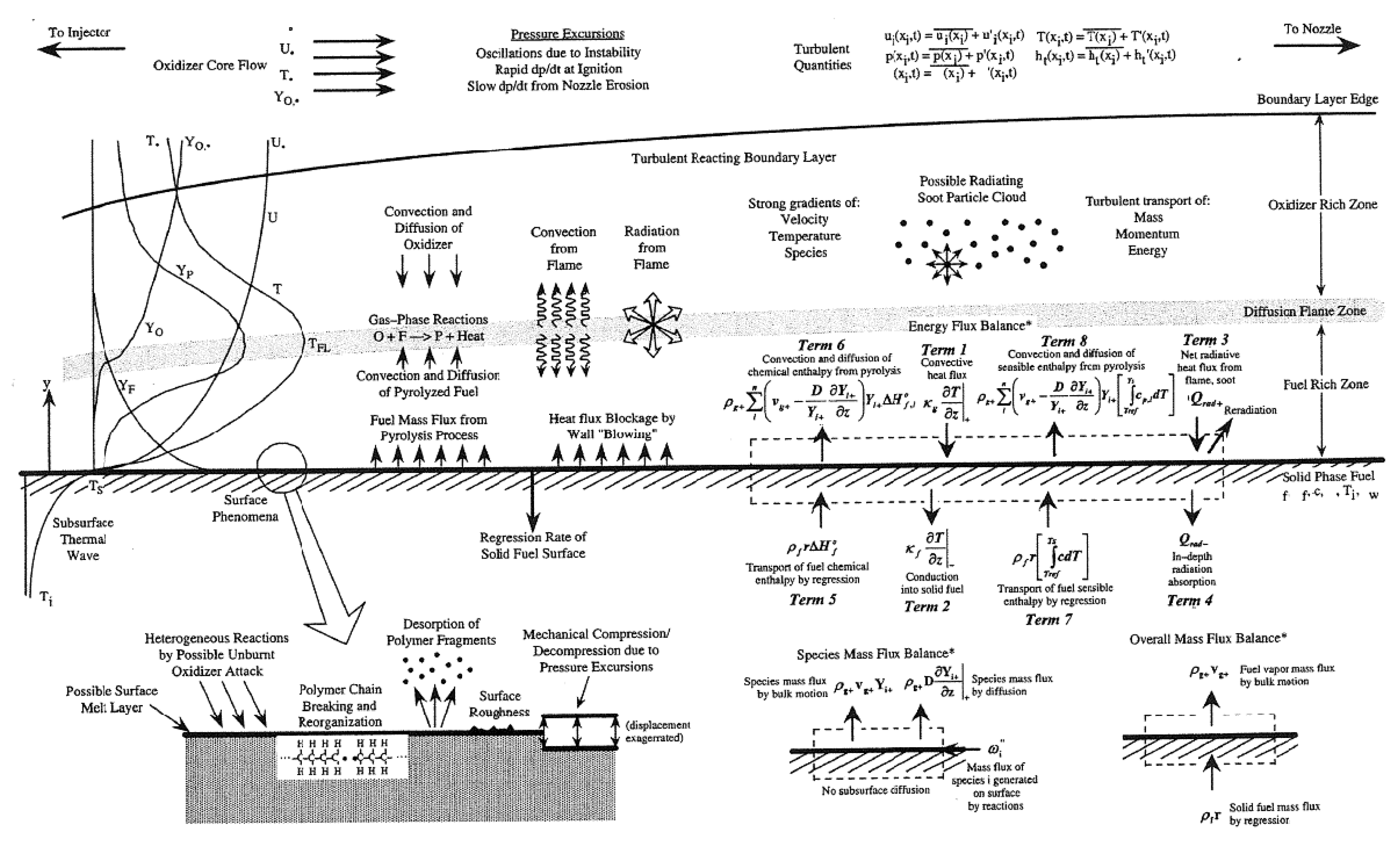
Chiaverini [
60] produced an excellent image representing the contribution of all the known mechanisms that play a role in the determination of the net heat flux that goes into the solid fuel (
Figure 1).
According to the above scheme, the conservation of mass and energy must be met in a control volume located right at the fluid–solid interface following the regressing surface.
The total mass balance + overall species conservation in such volume is therefore:
with
being the density,
v—the velocity,
—the mass flux,
—the regression rate,
,
and
, respectively—the mass diffusion, the concentration and the mass generation at the fuel surface of species
i. The subscript
g or
refers to the properties of the gas over the burning surface, while
f regards the solid fuel itself. The species conservation equation for species
i is instead:
Finally, the energy balance, considering the radiative heat transfer
as well, is:
with
where
and
are the specific enthalpy of formation of the fuel and of the species
i, respectively. Similarly,
c and
are the respective specific heats, which, integrated from the reference temperature
to the surface temperature
, give the sensible enthalpy. Finally,
is the thermal conductivity. As stated in Equation (
3), the first series of terms represents the energy entering the volume through regression, conduction and radiation, while the second series represents the energy released through convection, diffusion of species, conduction and radiation into the solid fuel. Applying the energy equation for the solid phase in the z (normal) direction, it is possible to calculate the thermal energy that is lost from the surface due to conduction through the fuel grain while assuming that there is little variation in the fuel thermal conductivity and specific heat capacity with respect to temperature. Mathematically, it can be written in the following way:
of which the general solution is:
where
and
are integration constants. Imposing the boundary conditions
and
the following exponential law can be derived:
From the above, the following equivalence is obtained by taking the first derivative at the fuel surface (
):
Additionally, the sensible contribution of fuel ablation in Equation (
3) can be rewritten as follows when using an average value of
c, as in Equation (
6):
Moreover, solid fuels are generally opaque (
) and all other radiation-related phenomena have been neglected to simplify the analysis
. Combining everything mentioned so far into Equation (
3), we obtain:
Simplifying some recurring terms, assuming the decomposition products being composed of only one species (now the subscript
i refers to the only decomposition product) and introducing the Equation (
1) into the above expression, the following can be obtained:
where
is the effective enthalpy of vaporization in
. In Equation (
12), a polynomial expression for
can be adopted and integrate numerically the sensible contribution.
The set of equations is completed by the pyrolysis kinetics, which allows to obtain the surface temperature by inverting the following expression:
where
A is the pre-exponential factor,
the activation energy and
the universal gas constant.
3. Reference Experimental Data
The numerical model was validated using experimental data from the University of Naples in Italy. Carmicino and Sorge have tested GOX-HDPE [
61,
62,
63] and GOX-HTPB [
64] hybrid rockets at lab scale. The choice of these particular test cases among the vast array of hybrids lab-scale testing described in literature was influenced by a number of factors:
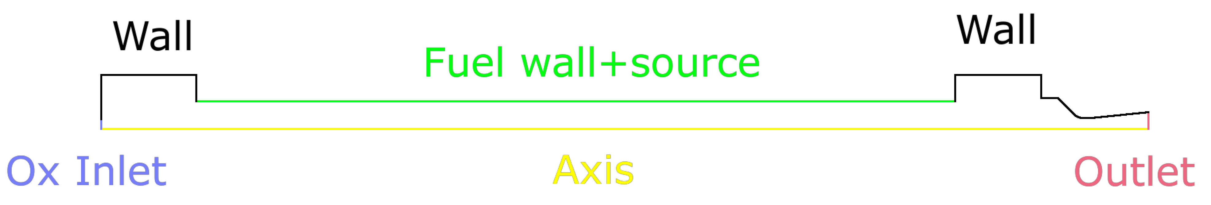
Engine geometrical configuration and general dimensions are fully recorded and it is possible to reconstruct the fluid domain into the CFD software;
Test results are well documented and span different operational conditions;
Motor and injector geometry is simple and straightforward to mesh. Moreover, the axis-symmetry of the problem has been exploited to build a 2D computational grid and save computational resources;
Oxidizer is injected into the combustion chamber in gaseous phase, so there is no need for a multi-phase simulation;
Fuels are classic hyrbid fuels and quite common in the literature, thus, their properties are well documented and reliable. Furthermore, HTPB and HDPE are not “liquefying fuels” (whose physics is more complex [
65,
66,
67,
68,
69]) and the mechanism of their pyrolysis can be modeled as a direct sublimation.
Table 1 and
Table 2 include all the average data used to perform the numerical validation. For more information on motor configuration, experimental findings and data processing, the reader is referred to the original papers. A useful discussion on regression rate averaging is provided in [
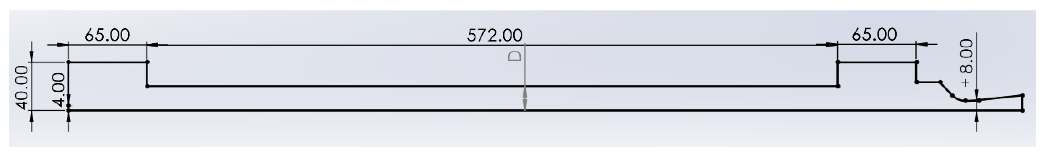
70]. Geometrical dimensions are highlighted in
Figure 2.
In relation to the experimental results just reported, it should be noted that, due to the unusual coupling between the oxidizer flow pattern at injection and the motor-internal geometry, the resulting average regression rate is strongly correlated with the port diameter history [
62]. Thus, in order to draw a proper comparison between experimental and numerical results, not only the correspondence of oxidizer mass flux but also that of the average regression rate must be considered.
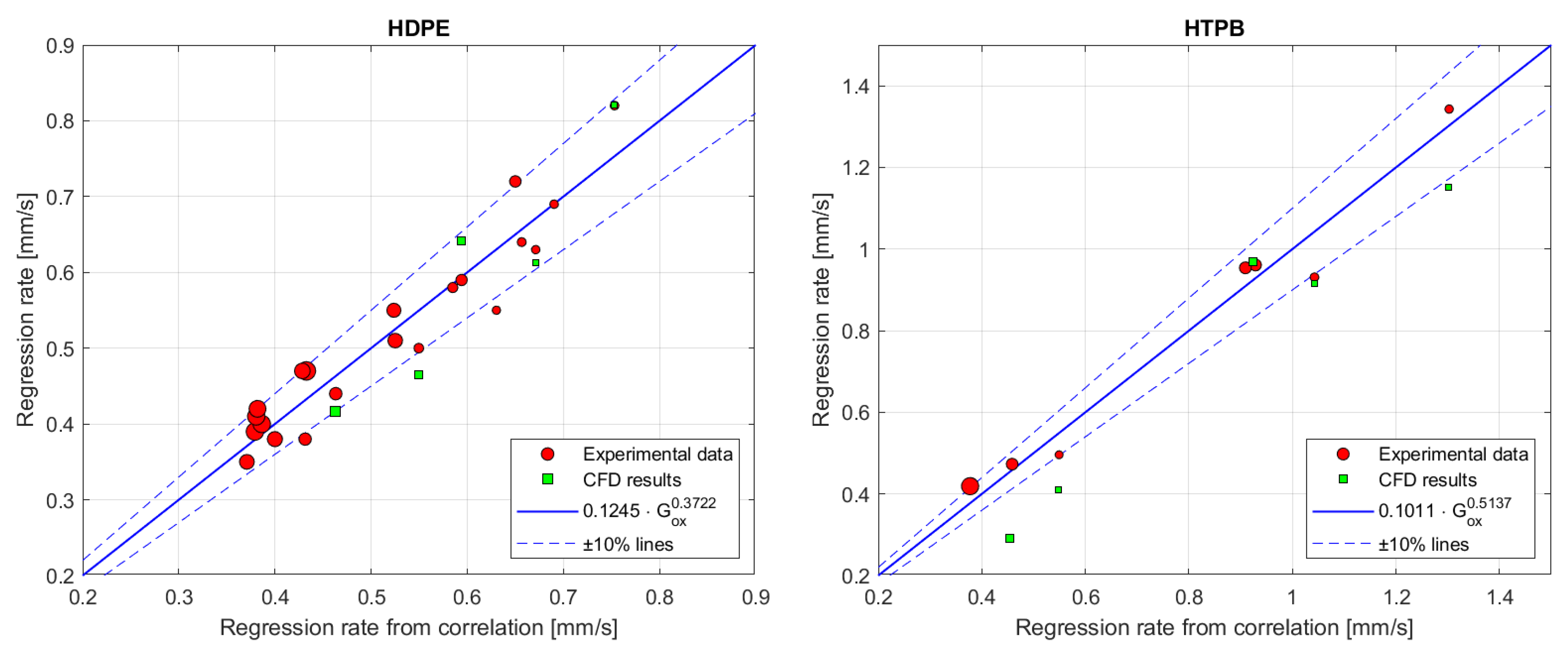
Figure 3 shows the data just presented and the corresponding extrapolated regression rate laws for both fuels.
4. Fuel Characteristics
Several physical factors about the solid fuel and its constituent monomer are required to solve the system of equations comprising Equations (
12) and (
13). Based on the expected heat flow and fuel surface temperature in a hybrid motor, C
H
(ethylene) and C
H
(1,3-butadiene) are regarded as the principal constituent monomers for HDPE and HTPB, respectively [
60,
71].
The physical characteristics needed to implement the model are then:
Solid fuel density: ;
Specific enthalpy of formation of fuel monomer: ;
Specific enthalpy of formation of solid fuel: ;
Specific heat capacity of fuel monomer ;
Arrhenius pre-exponential factor: A;
Energy of activation: .
Several sources in the literature provide these data. In general, all of the listed data for HDPE show satisfactory coherence, whereas data for HTPB show a significant variance and disagreement across the sources, particularly when it comes to the parameters of the Arrhenius equation and the specific enthalpy of formation of solid fuel [
71,
72,
73,
74,
75,
76]. This disparity can be explained by both the wide range of methodologies used to estimate the parameters [
60,
71] and the huge range of slightly different compositions that fall under the same category of HTPB.
NASA-Glenn and NIST databases [
76,
77] were used as references for HTPB thermochemical properties since they are comprehensive and reliable, whereas data provided by Chiaverini [
60] were used for the Arrhenius equation parameters.
Regarding Arrhenius equation parameters for HDPE, the activation energy was derived from the literature [
71], while a mean pre-exponential factor (generally A depends upon
, however, this dependence is negligible in most of the cases) has been obtained using the Lengellé approach [
71]:
where
is the Arrhenius pre-exponential factor in [1/s],
,
and
are, respectively, the average thermal diffusivity and the specific heat capacity of the fuel monomer in the temperature range of interest and
is heat of degradation (or pyrolysis) of the fuel, or, in other words, the heat necessary to transform the solid fuel into its associated gaseous monomer at
. Lastly,
is the remaining mass fraction of the polymer after the degradation, and it can be taken to be a small quantity (0.01).
Table 3,
Table 4 and
Table 5 contains all the numerical values of these parameters.
The density of the solid HTPB is taken as 930 kg/m
. The specific heat capacity for the gaseous monomer,
, is calculated as a fourth-order polynomial function of temperature for both HTPB and HDPE using the coefficients provided by NASA (NASA 9-Coefficient Polynomial Parametrization [
77]), which are also integrated in the CFD software database.
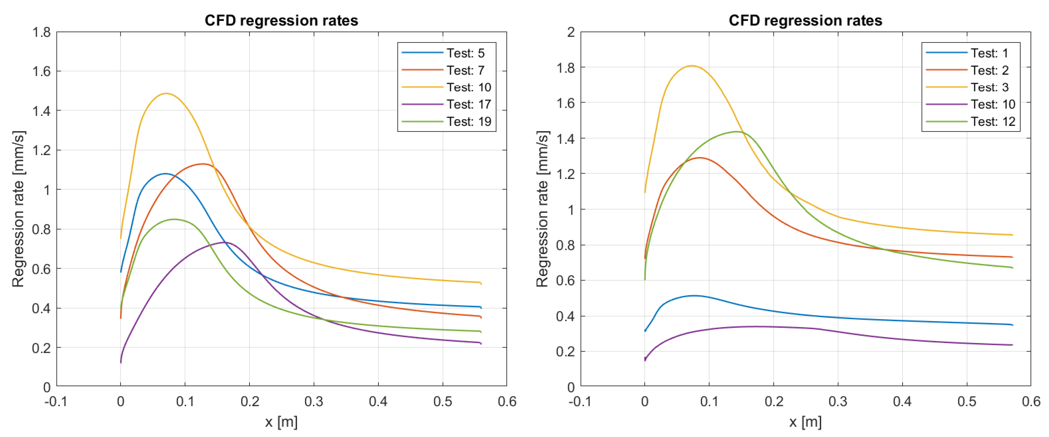
7. Regression Rate Comparison Analysis
It is worth noting that these two fuels seem to display quite different regression rates despite being somewhat similar in properties. Several attempts to improve the original Marxman model have been made [
75,
93,
94,
95], but a satisfactory explanation is still lacking. As shown in
Figure 15, the ratio
varies from 1.1 to 1.7, with potentially greater values for higher oxidizer mass fluxes. Moreover, taking as samples the simulation results of Test 5 and 2, which are comparable in terms of geometric features and oxidizer mass flux, it is possible to obtain
Figure 16,
Figure 17 and
Figure 18 as ratios of regression rates, effective vaporization enthalpy and fuel wall heat flux, respectively. The vaporization enthalpy
at the corresponding working point is about 20% lower for HTPB. This difference, as explained below, however, is not enough to account for the observed regression rate ratio according to Marxman’s classic hybrid rocket theory [
52,
53,
54].
Marxman’s theory states, indeed, that [
52]:
The ratio between HTPB and HDPE heat flux would be:
Given the similarity of the combustion chemistry of the two fuels,
can be assumed to be nearly equal, while the ratio between the blowing coefficient
B is proportional to the ratio of regression rates, producing the following expression:
Using the mean ratio obtained by the CFD simulation (
Figure 16), the results is completely off with respect to the observed one in
Figure 18, being even on the opposite direction. As noted before,
could not explain this discrepancy, as demonstrated by the expression below [
60], where again, the mean
ratio obtained though the CFD simulation of Test 5 and 2 (
Figure 17) is taken again:
Moreover, it is unlikely that radiation could account for a substantial portion of the difference, especially when considering that it is far more significant for low values of
G, while the regression rate ratio is diverging (
Figure 15). This discrepancy could also be the effect of other physical properties such as density of the solid fuel and Arrhenius constants. However, it seems very unlikely that they would result in such a strong difference, especially when accounting for all the negative feedback-loops that make hybrid rocket motors safe, but at the same time, cap the
of classic fuels to low values. The source of this effect should be researched further, and the density of the decomposition products in particular is suggested [
60]: lighter pyrolysis products may result in stronger blowing and blocking effects, resulting in the observed relationship between HDPE and HTPB. The primary breakdown species of a polymer is often its fundamental monomer. For the former, it is C
H
(ethylene), with a molecular mass of 28 g/mol. When compared to 54 g/mol of C
H
(1,3-butadiene) from HTPB, it is about twice as low. Furthermore, even if the decomposition gases are an heterogeneous mixture of very different species, the conservation of mass and atoms will produce a mean molecular mass that is around the fundamental monomer’s one (
Figure 19). An investigation of this effect through a rigorous analysis will be presented in future works.
8. Conclusions and Further Developments
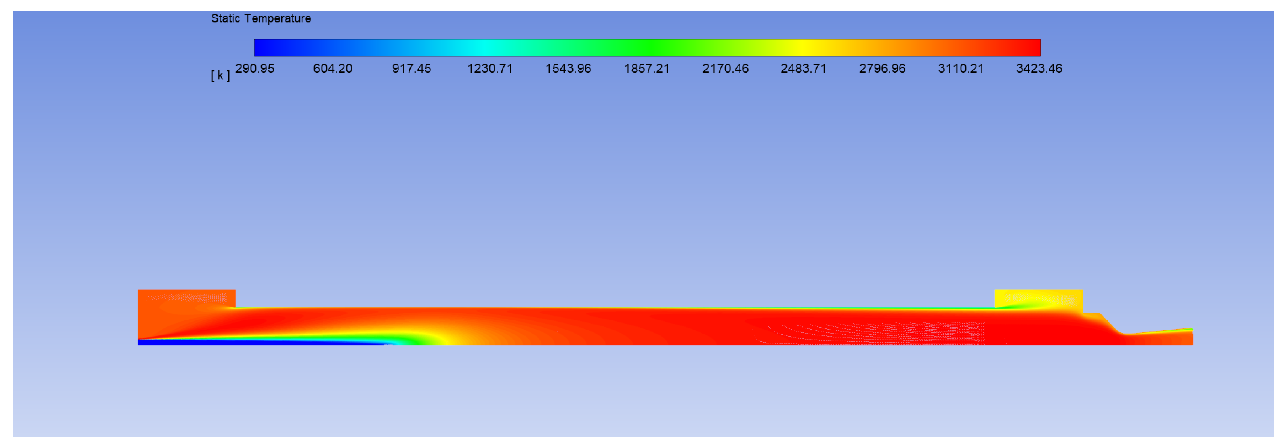
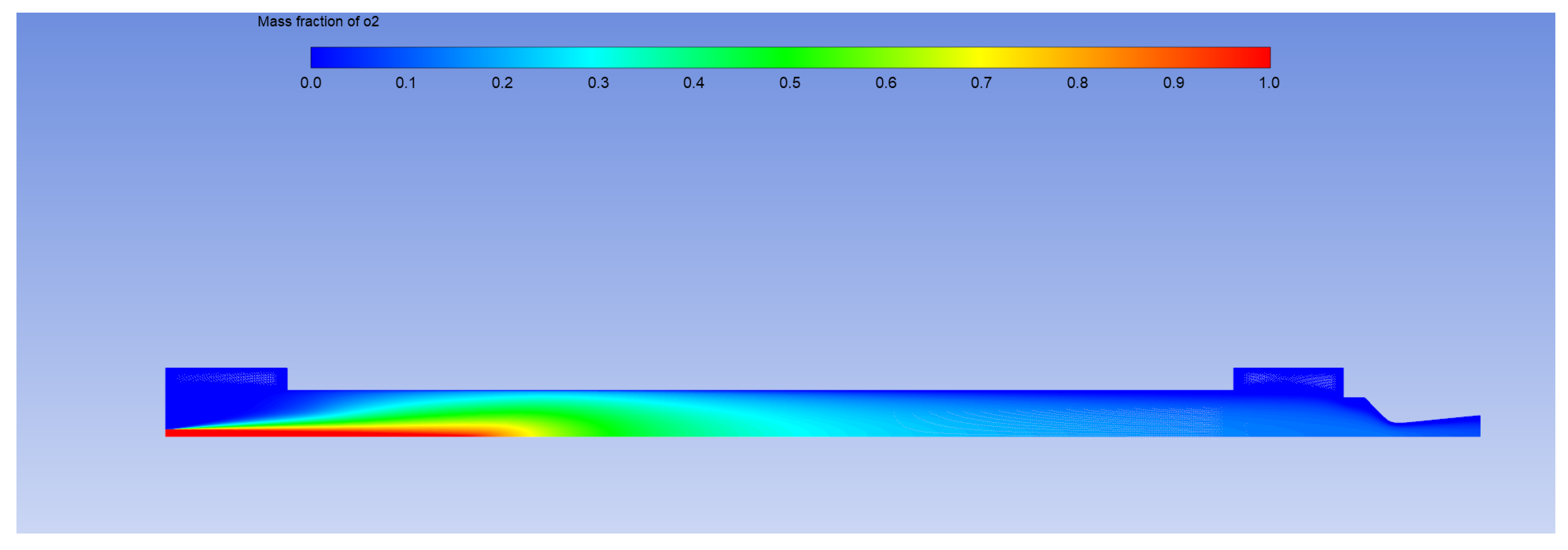
A numerical model of the ablation of classical polymeric fuels in hybrid rocket motors was implemented on a commercial CFD package using a special user-defined function that determines regression rate as a function of heat flux at the fuel surface, cell by cell. The regression rate was calculated by computing the surface energy balance in combination with the Arrhenius equation for fuel pyrolysis. A validation campaign using literature data from a cylindrical port-axial injection lab-scale motor was successfully completed. The propellant combinations GOX-HTPB and GOX-HDPE were utilized in the reference experiments, and gaseous oxygen was fed by a single hole injector. The numerically determined regression rate generally agrees within 10% of the experimental results for HDPE and 20% for HTPB, demonstrating the feasibility of tailoring a commercial software for the purpose, as well as the effectiveness, of a relatively simplified model in providing useful insight into the hybrid combustion process. CFD simulations enable the exploration of local processes inside the hybrid motor, which are frequently difficult to analyze in depth. Indeed, it has been demonstrated that a considerable local effect exists when the oxidizer flow impinges on the fuel surface, boosting the regression rate. The proposed CFD tool can be used to examine hybrid rocket regression rate behavior using parametric analysis, thus improving understanding of the ablation process and defining improved regression rate correlations. The addition of a suitable radiation model to the present UDF should improve the accuracy of the regression rate prediction, particularly for fuels that create considerable soot and/or at low oxidizer fluxes. Furthermore, it will be beneficial to adapt the model to non-classical fuels such as liquefying fuels (with the addition of an entrainment model) or fuels including energetic additions (e.g., metal particles). Finally, a discrepancy in the classic hybrid rocket theory was exposed regarding HDPE and HTPB regression rates. The proposed explanation is the difference in decomposition product density which lowers or increases the blowing effect. A detailed analysis will be conducted in future works to determine whether this effect could affect the boundary layer behavior and alter the convective heat transfer to the surface.


