Transport Barrier Triggered by Resonant Three-Wave Processes Between Trapped-Particle-Modes and Zonal Flow

Abstract

We address the mechanisms underlying low-frequency zonal flow generation in a turbulent system through the parametric decay of collisionless trapped particle modes and its feedback on the stabilization of the system. This model is in connection with the observation of barrier transport in reduced gyrokinetic simulations (A. Ghizzo et al., Euro. Phys. Lett. 119(1), 15003 (2017)). Here the analysis is extended with a detailed description of the resonant mechanism. A key role is also played by an initial polarisation source that allows the emergence of strong initial shear flow. The parametric decay leads to the growth of a zonal flow which differs from the standard zero frequency zonal flow usually triggered by the Reynolds stress in fluid drift-wave turbulence. The resulting zonal flow can oscillate at low frequency close to the ion precession frequency, making it sensitive to strong amplification by resonant kinetic processes. The system becomes then intermittent. These new findings, obtained from numerical experiments based on reduced semi-Lagrangian gyrokinetic simulations, shed light on the underlying physics coming from resonant wave-particle interactions for the formation of transport barriers. Numerical simulations are based on a Hamiltonian reduction technique, including magnetic curvature and interchange turbulence, where both fastest scales (cyclotron and bounce motions) are gyro-averaged.

1. Introduction

An important role of zonal flows (ZFs) in regulating turbulence and transport in tokamaks is now broadly accepted. The regime of near marginality [1] is not merely academically appealing as a paradigmatic model but it is of practical interest for its rich dynamics and for it allows the appearance of self-organization. Plasma turbulence differs in many ways from fluid turbulence and in tokamaks it is mostly driven by the free energy source of many micro-instabilities, essentially the gradients of density and temperature. In the core of the tokamak plasma, these micro-instabilities are driven by the ion temperature gradient (ITG) which concerns circulating ions. However when the frequency of the ITG mode falls below the ion bounce frequency, the dynamics of the ion trapped particles become important and one then speak of trapped ion modes (TIM). Another classes of instabilities driven by electrons are the electron temperature gradient (ETG) modes for circulating electrons but also the trapped electron modes (TEMs).

It is presently well known that turbulent transport in tokamaks is dominated by the ITG and TEM modes (see [2,3,4]). Early studies of plasma turbulence concerned drift-wave turbulence models, a reduced approach which clearly shows the generation of mesoscales structures such as zonal flows (ZFs), sheared flows. Motivated by the experimental discovery of a low-to-high (LH) transition in the plasma confinement, experimental and theoretical works in the two last decades have focused on whether the turbulence associated with the H-mode might be regulated by interactions with ZFs or shear flows. In particular the generation of zonal flow by finite beta drift waves or kinetic drift wave was investigated by Guzdar et al. in [5,6] showing the importance of parametric-type processes in the LH transition.

ZF dynamics are mesoscopic phenomena occurring at spatial scales in between the turbulence correlation length and the inverse characteristic gradient scale of the density profiles. ZFs may regulate and partially suppress drift-wave turbulence and associated transport. A simplified picture of such a phenomena was provided by the “predator-prey” model by Kim and Diamond [7] or Malkov et al. (2001) [8,9]. Based on a description of the coupled drift-wave turbulence ZF interaction, the model takes into account a population of drift-wave “quanta” (acting as prey), which grows through the linear ITG instability and feeds ZF (the predator) through the Reynolds tensor. Thanks to its relative simplicity, this model provide useful insight in the complex dynamics under investigation and in the dynamics of ZF. While considerable progress has been achieved in the understanding of the ZF physics (a review of physics ZF can be found in [10]), many aspects of the ZF dynamics remain nevertheless poorly understood.

When toroidal effects, such as magnetic curvature and $\nabla B$ drifts, are incorporated in the model and when a proper (reduced) kinetic treatment of trapped particles is used, the most prominent type of long wavelength micro-instabilities is collisionless TIMs (CTIMs) in the presence of a significant ion temperature gradient. CTIMs are a simple prototype of kinetic modes induced by the resonance of trapped ions with fluctuations through their precession motion. A major role in the complex interaction of ZFs and CTIM turbulence is expected to be played by mesoscopic non linear structures, which are called streamers, that result from the non linear dynamics of CTIM instabilities. Thus CTIMs introduce an alternate state dominated by oscillating low-frequency zonal flows (LFZFs) [11,12,13,14] near the critical temperature gradient threshold which can lead to a new type of intermittent dynamics where resonant kinetic processes may take place. Streamers are observed in numerical simulations studied in [15] and appear to be closely associated with avalanche type transport events [4]. While TIM turbulence contribute to enhance the transport owing to their radial elongation structures (non linear streamers) and thus to amplify the growth of ZF by resonance, the resulting LFZF is believed to be responsible for suppression fluctuations and stabilisation of turbulence. It has been shown in [16] that such LFZFs are key ingredients to trigger a bifurcation toward the generation of transport barriers.

A clear indication of the key role played by such LFZFs was the observation at the experimental advanced super-conducting tokamak (EAST) [17] of a low-frequency signal at a few kilohertz attributed to such LFZF, a signal which has been observed at a much lower frequency than the standard geodesic acoustic modes (GAMs) [18,19]. This brings us to an important question about the physical origin of these low-frequency oscillations while the usual ZF frequency is usually considered to be zero in the hydrodynamical approach, i.e., when excited by the standard Reynolds stress. Such LFZFs differ from the high-frequency GAMs. GAMs are not typically observed in the H mode plasma. From a physical point of view, GAM can be considered as an ion acoustic wave (IAW) in the geodesic version due to the magnetic geometry of the tokamak. On the experimental side, some of the defining GAM characteristics have been observed, including the occurring of a low frequency ZF counterpart [14,20,21,22]. The amplitude of such low frequency ZF was seen to increase with decreasing $r/a$, while the GAM intensity appears to decrease. Oscillations of electrostatic nature have been observed in the plasma edge at much lower frequency than the GAM in the EAST tokamak experiment [17]. The fluctuating potential power spectra exhibit a peak close to 2 kHz with two harmonics and with background peaking of 80kHz, while GAM does not appear to be active in the low-high transition under these experimental conditions. It was also reported that the frequency spectrum may exhibit more intermittent features. The existence of three-wave coupling between the turbulence in 80kHz and the low-frequency 2 kHz oscillations was also reported in this experiment. Similar behaviour was also reported in the ASDEX -Upgrade tokamak [20].

Moreover, more recently in [11], the authors have derived an analytical fluid model based on the use of a multiple spatio-temporal technique and ballooning modelling to study the growth of LFZF driven by direct phase modulation. This model allows recovering the concept of Blob-hole temporal structure [23] and the formation of two distinct mesoscopic structures referred, by the authors, as Caviton [24] (a region of strong reduced wave energy) and instanton [11,25] (a local temporal burst in the propagation of the energy).

In this article, by using a Hamilton-Jacobi formalism using action-angle variables, we focus on the physical mechanism which leads to the formation and the amplification of self-organised transport barriers (TBs) induced by the resonance with oscillating LFZF. While zero-frequency ZFs are quite non resonant, being relatively easy to drive up by the Reynolds stress, this new LFZF which results from toroidal geometry and kinetic effects, becomes then sensitive to a strong amplification driven by the resonant interaction between CTIM and CTEM provided that a polarisation source is high enough to generate an initial shear flow. In particular, we present numerical results obtained from the numerical integration of a reduced hamiltonian (Vlasov) gyrokinetic model for the trapped particle modes, and based on the action-angle model discussed in [12,13,26] and in Refs. [27,28,29] for two species. We address here the physical mechanisms responsible to strong amplification of ZF and the resulting TB’s formation. This paper is organized as follows. Basic equations of the trapped-particle model are presented in Section 2 while physical properties are recalled in Section 3. Issues related to the three-mode parametric decay are then addressed in Section 4. Numerical results relevant to the resonant growth of ZF are then presented in Section 5. Finally conclusion and future works are offered in Section 6.

2. Hamilton-Jacobi Model for Ion Temperature Gradient (Itg) Turbulence

The model, we consider here, describes the dynamics of trapped particle modes (TPMs) in which the gradients of temperature provide the source of free energy (the density gradient being zero initially without polarization source). TPMs have been obtained by gyro-averaging the particle dynamics over fast scales i.e., over the cyclotron frequency ${\omega }_{cs}$ and bounce ${\omega }_{bs}$ motions in the toroidal geometry, where the index s refers to the considered species $s=e,i$ for electrons or ions respectively. This task is made easier in the framework of the Hamiltonian- Jacobi formalism using action- angle variables (see the works of [26,30] or more generally of [31,32]). Due to their curvature drift, the orbits of trapped ions exhibit “banana” shape centred on the low magnetic field side. The low-frequency response for TPM is obtained by making a phase-angle average over the cyclotron phase and the bounce motion leading to invariance of the total energy $E_s=\frac{1}{2}{m}_s{v}_{G\Vert s}^2+{\mu }_{s}B\left({\mathit{x}}_{Gs}\right)$ and of the so-called adiabatic invariant ${\mu }_s=m_s{v}_{G\perp s}^2/2B\left({\mathit{x}}_G\right)$, where $v_{G\perp s}$ is the perpendicular velocity.

Here the label G is a conventional notation which refers to the guiding centre and ${\mathit{x}}_G$ refers to $\left(r,\theta \right)$ polar coordinates. In agreement with the experimental conditions, we consider low beta values and a poloidal field $B_{\theta }$ lower than the toroidal magnetic field $B_{\phi }$. Here the modulus of the magnetic field is given by $B\left(r,\theta \right)=B_{0}b\left(\theta \right)=B_0\left(1+\epsilon si{n}^2\frac{\theta }{2}\right)$ where $B_0$ is the minimal value of the magnetic field amplitude B at $\theta =0$ ($R=R_0$ being then the major radius and $r=r_0$ the minor radius). In this configuration the poloidal flux is linked to the poloidal field by $d\psi =-B_{\theta }{R}_{0}dr$ and $B_{\theta }/B=\epsilon /q\left(r\right)$ where q is the safety factor. Here $\epsilon =r/R_0$ is the inverse aspect ratio.

Rather than working with the adiabatic invariant ${\mu }_s$, it was interesting to introduce the pitch angle parameter ${\kappa }_s$ defined by the relation ${\kappa }_s^2=\left(1-{\lambda }_s\left(1-\epsilon \right)\right)/2\epsilon {\lambda }_s$ where ${\lambda }_s={\mu }_s{B}_0/E_s$. Particle trapping occurs when ${\lambda }_{s,min}\le {\lambda }_s\le {\lambda }_{s,max}$ while particles are passing if $0\le {\lambda }_s\le {\lambda }_{s,min}$ where ${\lambda }_{s,min}=1/\left(1+\epsilon \right)$ and ${\lambda }_{s,max}=1/\left(1-\epsilon \right)$. Thus particles are passing if $1\le {\kappa }_s<+\infty$ and trapped if $0\le {\kappa }_s<1$. The parallel velocity takes then the following form:

$$v_{G\Vert s}={\epsilon }_{\Vert }{v}_s{\left(\frac{2\epsilon }{2\epsilon +\left(1-\epsilon \right){\kappa }_s^{-2}}\right)}^{\frac{1}{2}}{\left(1-{\kappa }_s^{-2}si{n}^2\frac{\theta }{2}\right)}^{\frac{1}{2}}$$

where $v_s=\sqrt{2E_s/m_s}$ and ${\epsilon }_{\Vert }$ is the sign of the parallel velocity. For passing particles, the integrals over $\theta$ run over the interval $\left[0,\pi \right]$ using up-down symmetry. It is then convenient to introduce the change $\vartheta =\frac{\theta }{2}$, which spans $\left[0,\frac{\pi }{2}\right]$ to obtain the Elliptic functions. For trapped particles, where ${\kappa }_s=sin\frac{{\theta }_0}{2}$, it is better to introduce the change of variable $sin\vartheta ={\kappa }_s^{-1}sin\frac{\theta }{2}$ where the new variable $\vartheta$ spans $\left[0,\frac{\pi }{2}\right]$.

We restrict our approach to identical classes of solutions of trapped particles keeping the same parameter $\kappa$ for both electron and ion populations. We have assumed here that this dependency is realised in the amplitude term of the bounce frequency, thus the quantity ${\overline{\omega }}_b\left(\kappa \right)$ is taken identical for both species of particles. Following the work of Kadomtsev and Pogutse in [33,34], the bounce and precession frequencies are given respectively by the following relations:

$${\omega }_{bs}=\sqrt{\frac{2E_s}{m_s}}\frac{1}{q_0{R}_0}{\overline{\omega }}_b\left(\kappa \right)\mathrm{with}{\overline{\omega }}_b\left(\kappa \right)\simeq \frac{\pi \sqrt{\epsilon }}{2\sqrt{2}K\left(\kappa \right)}$$

(1)

$${\omega }_{ds}{E}_s=\frac{q_0{E}_s}{e_s{r}_0{R}_0{B}_0}{\overline{\omega }}_d\left(\kappa ;S\right)$$

(2)

$${\overline{\omega }}_d\left(\kappa ;S\right)=\frac{2E\left(\kappa \right)}{K\left(\kappa \right)}-1+4S\left(\frac{E\left(\kappa \right)}{K\left(\kappa \right)}+{\kappa }^2-1\right)$$

(3)

where $S=\frac{r_0}{q_0}{\left(\frac{dq}{dr}\right)}_{r_0}$ is the magnetic shear. $K\left(\kappa \right)$ and $E\left(\kappa \right)$ are the complete elliptic integrals of the first and second kind respectively.

Trapped particles are described by two invariants $E_s$ and $\kappa$ and by the distribution function $f_s=f_{E_s,\kappa }\left(\psi ,\alpha ,t\right)$ where $\alpha =\phi -q_0\theta$ is the precession angle and $\psi$ the poloidal flux. The distribution function $f_s$ for the species s (with $s=e,i$ for electrons and ions respectively) in banana orbits fulfils the Vlasov equation:

$$\frac{\partial f_s}{\partial t}+{\omega }_{ds}\left(\kappa ;S\right)E_s\frac{\partial f_s}{\partial \alpha }+\left[J_{0s}\varphi ,f_s\right]={\partial }_{\psi }\left(D\left(\psi \right){\partial }_{\psi }{f}_s\right)$$

(4)

with the advective-term depending on the gyro-average operator $J_{0s}$. The model consists of solving $N_{E_s}$ times $N_{\kappa }$ Vlasov equations in a parallel way coupled nonlinearly by the quasi-neutrality equation. Here $N_{E_s}$ and $N_{\kappa }$ denote the number of values for “sampling” the parameters $E_s$ and $\kappa$ respectively.

Here $\left[.,.\right]$ denotes the standard Poisson bracket which reads as

$$\left[J_{0s}\varphi ,f_s\right]={\partial }_{\psi }\left(J_{0s}\varphi \right){\partial }_{\alpha }{f}_s-{\partial }_{\alpha }\left(J_{0s}\varphi \right){\partial }_{\psi }{f}_s$$

(5)

This gyro-average operator $J_{0s}$ introduces a “banana” scale ${\delta }_{bs}$ corresponding to the width of the particle’s trajectory in the $\psi$ direction, while the gyro-phase average on the Larmor radius ${\rho }_{cs}$ acts along the direction of the precession angle $\alpha$. Here $J_{0s}$ was approximated by the Pade’s relation giving to:

$$J_0={\left(1-\frac{E_s}{4}{\delta }_{bs}^2{\partial }_{\psi }^2\right)}^{-1}{\left(1-\frac{E_s}{4}\frac{{\rho }_{cs}^2}{a^2}{\partial }_{\alpha }^2\right)}^{-1}$$

(6)

The Vlasov Equation (4) is then coupled, in a self-consistent way, with the quasi-neutrality condition $\delta n_e\simeq \delta n_i$ which becomes here

$$C_e\left(\varphi -{〈\varphi 〉}_{\alpha }\right)-C_i\left(1+\frac{m_e}{m_i}\right)\overline{▵}\varphi =\sum _{s=e,i}sgn\left(e_s\right){\overline{n}}_s$$

(7)

where ${\overline{n}}_s$ is the gyro-averaged density of species s. Here the operator, which indeed describes polarization effects, is given by

$$\overline{▵}\simeq q_0^2{\rho }^{\ast 2}{\partial }_{\alpha }^2+{\delta }_{bi}^2{\partial }_{\psi }^2$$

(8)

which introduces different spatial scales. In (6) we have introduced the normalized quantities $\frac{{\rho }_{cs}}{a}=\sqrt{\frac{T_s{m}_s}{T_i{m}_i}}$ with ${\rho }^{\ast }=\frac{{\rho }_{ci}}{a}$. The polarization effects have been taken into account in the quasi- neutrality equation by the introduction of the polarization density (the Laplacian term). In (7), $C_e$ and $C_i$ are constants accounting for the fraction of trapped particle $f_p$ (here assumed to be identical for both trapped populations) and we have finally

$$C_e=\left(1+{\tau }^{-1}\right)/f_p\mathrm{and}{C}_i=C_e{f}_p\tau$$

(9)

where $\tau =T_e/T_i$ is the ratio of the electron to the ion temperature. The first term in Equation (7), in the left hand side (lhs), comes from the adiabatic condition of circulating electrons while the second term is due to the polarization charge. We define by $n_s$ the density of species s by the relation

$$n_s\left(\psi ,\alpha ,t\right)={\int }_0^{1}d\kappa \kappa K\left(\kappa \right)\frac{2}{\sqrt{\pi }}{\int }_0^{+\infty }d{E}_s\sqrt{E_s}{f}_{s;\kappa ,E_s}\left(\psi ,\alpha ,t\right)$$

(10)

and ${\overline{n}}_i$ is the gyro-averaged density obtained from Equation (10) by replacing the distribution $f_s$ by $J_{0s}{f}_s$. Finally trapped ion turbulence develops on length scale of the order of the banana width ${\delta }_{bi}$ and time scale determined by ${\omega }_{d0}^{-1}$ where ${\omega }_{d0}=q_0{T}_0/e_i{r}_0{R}_0{B}_0$. Here ${\delta }_{bs}$ is constant since we have neglected the dependence in $\kappa$ and is found close to ${\rho }_{cs}{q}_0/\sqrt{\epsilon }$. Notice that for electrons the sign of ${\omega }_{de}$ is negative. In all simulations presented here, the diffusion coefficient $D\left(\psi \right)$ is zero everywhere excepted in a small region (5% of the total space) on the boundary limit in the poloidal flux to maintain the stability of your numerical scheme when strong turbulence emerges. Such approach is kinetic in nature and can be reduced to the Hasegawa- Wakatani in a two-field model (see [35] for more details).

3. Physical Properties of the Tpm Model

3.1. Lfzf Driven by the Interchange Turbulence

The LFZF can play a key role in the dynamical interaction among ZFs, streamers and shear flows generated by the interchange turbulence. In [16] we have studied the role of this component which can trigger a transition by regulating the turbulence provided that the LFZF is sufficiently amplified. While the emergence of the LH transition requires the gyrokinetic simulation of flux-driven forcing, we adopt here an initial value problem without source term in the Vlasov equations. Within the framework of a simplified picture of the turbulence involving ITG instabilities (restricted here to the study of trapped particle modes), many actors are implicated such as collisionless TIMs, streamers and of course zonal flows. Notice that near the instability threshold the system may also evolve onto a globally organised state dubbed the $E\times B$ staircase [36,37]. This is a self-organised state characterized by the containment of avalanche activity, which is detrimental to confinement, by a series of micro-barriers for transport, i.e., the staircase picture, which is beneficial for confinement. Such a marginal equilibrium state provides (while segregating regions where avalanching is dominant from regions where zonal flow concentrates in micro-barrier) a natural and dynamic means for both antagonistic trends to simultaneously exist. It is in fact a spatio-temporal version of the phenomenon met in the simplified time-varying predator-prey model. We start by summarising here below some of the results of calculations published in [12,13,30] concerning the physical properties of LFZF.

In the framework of CTIM, a new trapped-particle-induced ZF mode is shown to appear at very low frequency close to the ion precession frequency ${\omega }_{d0}$ (here referred as the LFZF). The nature of the zonal flow is indeed modified due first to the toroidal geometry and secondly to kinetic trapping effects driven by the TIM turbulence. It is then possible to connect the temporal oscillations of the zonal flow component to the evolution of the mean electric potential ${〈\varphi 〉}_{\alpha }$ which is now described by the following equation:

$$\frac{\partial {〈\varphi 〉}_{\alpha }}{\partial t}={〈\frac{\partial \delta \varphi }{\partial \psi }\frac{\partial \delta \varphi }{\partial \alpha }〉}_{\alpha }-\frac{3T_i}{8T_0{C}_i}{〈\frac{\partial \delta P_i}{\partial \psi }\frac{\partial \delta \varphi }{\partial \alpha }+\frac{\partial \delta P_i}{\partial \alpha }\frac{\partial \delta \varphi }{\partial \psi }〉}_{\alpha }+\frac{T_i}{4T_0{C}_i}\frac{\partial {〈\delta Q〉}_{\alpha }}{\partial \psi }$$

(11)

assuming that there is no dissipation (i.e. $D\to 0$) and where

$${〈\delta Q〉}_{\alpha }={\int }_0^{2\pi }\frac{d\alpha }{2\pi }\frac{3}{2}\delta P_i\left(-\frac{\partial \delta \varphi }{\partial \alpha }\right)$$

(12)

In Equation (11) the first term in the second member denotes the Reynolds tensor, while the two following terms are a straightforward consequence of the interchange turbulence induced and polarization effects. The third term on the rhs of Equation (11) is linked to the heat flux ${〈\delta Q〉}_{\alpha }$ defined by Equation (12) and where $\delta A$ denotes the fluctuating perturbations of the quantity A.

It must be pointed out that the effect of the Reynolds tensor has been recently reproduced in the recent work of Y.Z. Zhang et al. in [11] based on a multiple scale technique applied to the Braginskii’s fluid model when the toroidal geometry is included. This approach reveals that ZF becomes a local travelling wave, associated with the emergence of mesoscopic structures as two cavitons followed by instantons. These terms have a somewhat different meaning from the original use in quantum electrodynamical (QED) theory. Cavitons are associated with local spatial region of energy depression while instantons refer to local peaks (see Refs. [24,25] for more details).

Since TIMs are unstable when ${\omega }_{\ast i}/{\omega }_{d0}\sim \nabla P_i.\nabla n_i>0$ (where ${\omega }_{\ast i}$ is the ion diamagnetic frequency), these modes are analogous to interchange modes. They can lead to a modification of the pressure profile and in particular of the mean ion pressure. Thus the temporal evolution of ${〈\varphi 〉}_{\alpha }$ is associated with the following equation:

$$\frac{\partial {〈P_i〉}_{\alpha }}{\partial t}=-{〈\left[\delta \varphi ,\delta P_i\right]〉}_{\alpha }-\frac{2}{3}{\partial }_{\psi }{〈\left[\overline{▵}\delta \varphi ,{\partial }_{\alpha }\delta M_{2i}\right]〉}_{\alpha }+{\partial }_{\psi }\left(D\left(\psi \right){\partial }_{\psi }{〈P_i〉}_{\alpha }\right)$$

(13)

indicating that it is the non-adiabacity between $\delta P_i$ and $\delta \varphi$ which drives non-linearly a modification of the mean pressure ${〈P_i〉}_{\alpha }$. Thus for $J_0\to 1$ and considering ${\delta }_{bi}\ll 1$, Equation (13) reduces to:

$$\frac{\partial {〈P_i〉}_{\alpha }}{\partial t}\simeq -{〈\left[\delta \varphi ,\delta P_i\right]〉}_{\alpha }+{\partial }_{\psi }\left(D\left(\psi \right){\partial }_{\psi }{〈P_i〉}_{\alpha }\right)$$

(14)

In Equation (14) we have introduced the moment $M_{ni}$ of $n-$order defined by:

$$M_{ni}=\psi {\omega }_{d0}{\int }_0^{1}d\kappa \kappa K\left(\kappa \right){\overline{\omega }}_d\left(k;s\right)\frac{2}{\sqrt{\pi }}{\int }_0^{+\infty }d{E}_i{\sqrt{E}}_i{E}_i^n{f}_{\kappa ,E_i,i}$$

(15)

3.2. Shear Flow Generation by Polarisation Effects

Polarization effects are intimately associated with the process of Hamiltonian reduction technique used in the gyrokinetic modelling as shown in Ref. [38]. In the guiding centre model the drifting motion of a gyrating charged particle in crossed electric and magnetic fields leads to a “polarization shift” from the guiding-center position in comparison with the particle location of the real particle. Thus the gyrokinetic theory retains the polarization correction in its quasi-neutrality Equation (7) through the introduction of a Laplacian term $\overline{▵}\varphi$. For illustrative purposes we have recently analysed in detail the dynamical evolution of the mean electric potential, which characterizes the zonal flow. Such analysis yields to Equation (11), where the polarization effects have been taken into account. From Equation (11) we can obtain some indication concerning these polarization effects on the modification of the zonal flow since only the first term in (11) represents the Reynolds tensor while the two other terms (the anticommutator and the heat flux derivative ${\partial }_{\psi }{〈\delta Q〉}_{\alpha }$) are driven by the polarization term. Basically the introduction of polarization effects can modify the nature of the zonal flow. Here we have adopted to modify the initial condition of the distribution function (by introducing a perturbed equilibrium allowing injection of heat into the system) while keeping identical the parameter $C_i$ in time.

Shear flows are likely key ingredients for triggering bifurcations which lead to the formation of transport barriers. Indeed a recent work [39] using vorticity injection in flux-driven gyrokinetic simulations has shown the formation of a TB in a self-consistent way. This work has shown that for sufficiently large shearing rates, turbulent transport can be suppressed and a TB builds up. However the plasma polarisation may imply the development of a temperature anisotropy which leads to the excitation of ITG modes. The resulting modes contribute to the Reynolds stress that screens the induced sheared electric field. Thus turbulence and its associated zonal flows are generated in the vinicity of the barrier destabilizing the latter due to the screening of the polarisation source by ZFs. These gyrokinetic simulations were performed in a low collisionality regime, which is in the so-called banana regime relevant to the ITER device. This assumption ensures first that collisions do not play a critical role here, and second, that CTIMs may play a key role in the mechanism of TB formation. Moreover, resonant modes can also significantly grow and modify the transport properties. We have modified the equilibrium condition to take into account the injection of polarisation. Let us consider for instance the following equilibrium

$$F_{0s}\left(\psi \right)=\left(1-n_{0s}\right)F_{eq,s}\left(E_s\right)+n_{0s}{g}_{0s}\left(E_s,\psi \right)$$

(16)

where $F_{eq,s}\left(E_s\right)=T_s^{-3/2}{e}^{-E_s/T_s}$ and

$$g_{0s}\left(E_s,\psi \right)=T_{es}^{-3/2}{e}^{-\frac{E_s}{T_s}}\left[1+\Delta \tau {\omega }_d\left(\kappa ;S\right)\left(\frac{E_s}{T_s}-\frac{3}{2}+\beta \right)\psi \right]$$

(17)

From (4) we see that the distribution $F_{eq,s}$ is a global (Maxwellian) equilibrium which satisfies the Vlasov equation for $J_0\varphi =0$. Thus the perturbation term $g_{0s}\left(E_s,\psi \right)$ in (16) can also be interpreted as a (secondary) marginal equilibrium which also satisfies the Vlasov Equation (4) provided that the diffusion coefficient $D\left(\psi \right)$ is zero.

For instance, in the case of one species only (the so-called trapped-ion modes) the non linear counterpart of the perturbation, $g=g_{E_i,\kappa }\left(\psi ,\alpha ,t\right)$, must also satisfy the non linear system formed of $N_{E_i}{N}_{\kappa }$ Vlasov-type equations, parametrized by the two adiabatic invariants $E_i$ and $\kappa$ in the following form:

$$\frac{\partial g}{\partial t}+{\omega }_{di}\left(\kappa ;S\right)E_i\frac{\partial g}{\partial \alpha }+\left[J_{0i}\varphi ,g\right]={\partial }_{\psi }\left(D\left(\psi \right){\partial }_{\psi }g\right)$$

(18)

coupled with the quasi-neutrality condition:

$$C_e\left(\varphi -{〈\varphi 〉}_{\alpha }\right)-C_i\overline{▵}\varphi ={\overline{n}}_i\left[g\right]-n_0$$

(19)

We can also define a pseudo-density of the particle species $s=i$ by using Equation (10). By renormalizing g such that its mean density $n_0$ is equal to one, we see that g satisfies the initial system given by Equations (4) and (7). Thus the distribution g can be viewed as a second equilibrium attainable from $F_{eq}\left(E_i\right)$ from a transition or bifurcation process. Here the parameter $\beta$ corresponds to the injection of polarisation and is connected to the quasi-neutrality condition by

$$C_e\left(\varphi -{〈\varphi 〉}_{\alpha }\right)-C_i{\delta }_{bi}^2\frac{d^2\varphi }{d{\psi }^2}={\overline{n}}_i\left[g\right]-n_0$$

(20)

or equivalently, when applying the gyro-average operator ${〈.〉}_{\alpha }$ on (20) we obtain

$$C_i{\delta }_{bi}^2\frac{d^2{〈\varphi 〉}_{\alpha }}{d{\psi }^2}=\chi \left(1+\beta {〈{\omega }_d〉}_{\kappa }\Delta \tau \psi \right)-1$$

(21)

where $\chi$ is a renormalisation constant defined by

$$\chi =\frac{1}{1+\frac{\beta \Delta \tau }{2}{〈{\omega }_d\left(\kappa ,S\right)〉}_{\kappa }}$$

(22)

Integrating (21) over the variable $\psi$ leads to the following expression

$$C_i{\delta }_{bi}^2\frac{d{〈\varphi 〉}_{\alpha }}{d\psi }=\psi \left(1-\chi -\chi \beta {〈{\omega }_d〉}_{\kappa }\Delta \tau \frac{\psi }{2}\right)$$

(23)

and finally to

$$C_i{\delta }_{bi}^2{〈\varphi 〉}_{\alpha }=\left(1-\chi \right)\frac{{\psi }^2}{2}-\chi \beta {〈{\omega }_d〉}_{\kappa }\Delta \tau \frac{{\psi }^3}{3}$$

(24)

Here we have $\frac{d{〈\varphi 〉}_{\alpha }}{d\psi }=0$ for $\psi =0$ or 1,

$$\begin{array}{c}{C}_i{\delta }_{bi}^2{〈\varphi 〉}_{\alpha }=0\mathrm{for}\psi =0\\ C_i{\delta }_{bi}^2{〈\varphi 〉}_{\alpha }=\frac{\beta {〈{\omega }_d\left(\kappa ;S\right)〉}_{\kappa }\Delta \tau }{12\left(1+\beta {〈{\omega }_d\left(\kappa ;S\right)〉}_{\kappa }\frac{\Delta \tau }{2}\right)}\mathrm{for}\psi =1\end{array}$$

(25)

To help as understand how the self-organized structures are formed, we will display the expression of ${〈\varphi 〉}_{\alpha }$ (shown in solid line in Figure 1) and its first derivative $\frac{d{〈\varphi 〉}_{\alpha }}{d\psi }$ (in dotted line in Figure 1). Alternatively, we have also plotted the quantity $g_0\left(E_i,\psi =0.5\right)-T_i^{-\frac{3}{2}}exp\left(-\frac{E_i}{T_i}\right)$ as a function of the energy $E_i$ in Figure 2, for different values of the parameter $\beta$, here the energy $E_i$ being normalized to a ion reference temperature $T_0$. One cannot fail to notice the correlation between the caviton-type solution of [11] and possible zonal flow associated with energy depression.

3.3. Propagating Blob-Hole Solution

In order to explore whether self-organized structures -and in particular the Blob-hole pattern, that is a simplified version of the staircase phenomenon observed in refs. [36,37]—can emerge in such system, a numerical simulation has been performed using the initial condition $g_{0s}\left(E_s,\psi \right)$ given in (17) with a perturbation given by

$$\delta f_s=T_s^{-\frac{3}{2}}{e}^{-\frac{E_s}{T_s}}\delta {\varphi }_{max}▵\tau sin\left(\pi \psi \right)cos\left(n\alpha \right)$$

(26)

The perturbation is made on mode $n=5$ with an amplitude of $\delta {\varphi }_{max}={10}^{-4}$ to start the instability. We have used a phase space sampling of $N_{\alpha }{N}_{\psi }=513\times 257$ for $N_{\kappa }{N}_E=16\times 128$ different Vlasov equations coupled together from the quasi-neutrality condition. We haven taken here $▵\tau =0.15$, $C_e=0.10$, $C_i=1$, an ion banana width of ${\delta }_{bi}=0.0936$ and a ion Larmor radius of ${\rho }_{ci}=0.01$ (to simplify the presentation of results, identical values for the electron species have been considered here, however we have checked that considering smaller values of these quantities does not modify the results in a fundamental way). The magnetic shear is $S=2$.

Figure 3 and Figure 4 show the emergence of the blob-hole pattern in both potential $\varphi$ and the first moment of the distribution $g_s$ using (15), at two different times $t{\omega }_{d0}=4.6$ and $t{\omega }_{d0}=9.6$. On the one hand, suppression of turbulence is only observed in hole region (due to the presence of a strong zonal flow) while strong peaks have been also observed in turbulent region, as the result of emergence of a non linear activity. The first plot, at time $t{\omega }_{d0}=4.6$, displays the appearance of a strongly non linear mesoscale structure which illustrates a feature of the shear flow generation driven by the Reynolds stress. Suppression of turbulence and transport by sheared flow takes place progressively by reducing the size of the turbulent region (located in the blob region). The phase space pattern is linked to the excitation of the shear flow driven by the polarisation. It can also be noted that the stabilization of the system is accompanied by a gradual decrease in the size of turbulent mesoscopic structures and ultimately results in the emergence of a global ZF.

The results of the previous simulation show that propagating solutions may play a major role in the system as already mentioned in [11]. Let us consider a system composed of only one mobile species, say ions with a population of adiabatic electrons to simplify the presentation. In this case it is possible to find a marginal solution of the Vlasov quasi-neutrality system for which the Hamiltonian H writes $H={\omega }_k\left(\kappa ;S\right)E_i\psi +J_0\varphi$. Looking for stationary solutions of the form $g=g_{E,\kappa }\left(\psi ,\alpha -\omega t\right)$ and $\varphi =\varphi \left(\psi ,\alpha -\omega t\right)$, the Vlasov Equation (18) reads also

$$\left[\left({\omega }_k\left(\kappa ;S\right)E_i-\omega \right)\psi +J_0\varphi ,g\right]=0$$

(27)

and ${\omega }_{CTIM}=\frac{3}{2}n{\omega }_d\left(\kappa ;S\right)$ at the threshold of the ITG instability. Thus using the boundary conditions

$$\begin{array}{c}{g}_{E,\kappa }=T_i^{-\frac{3}{2}}{e}^{-\frac{E_i}{T_i}}\mathrm{for}\psi =0\\ g_{E,\kappa }=T_i^{-\frac{3}{2}}{e}^{-\frac{E_i}{T_i}}\left[1+\Delta \tau {\omega }_d\left(\kappa ;S\right)\left(\frac{E_i}{T_i}-\frac{3}{2}\right)\right]\mathrm{for}\psi =1\end{array}$$

(28)

a solution satisfying the Vlasov equation is then obtained and finally we recover the solution given in (17) by taking $\beta =0$.

Moreover by applying the standard linear analysis of Landau on the Vlasov Equation (18) and by considering perturbation in the form $\delta g_n\left(\psi \right)e^{i\left(n\alpha -\omega t\right)}$ and $\delta {\varphi }_n\left(\psi \right)e^{i\left(n\alpha -\omega t\right)}$ on the distribution function and the electric potential respectively, one obtains the following condition (assuming the polarization term negligible in first approximation):

$$C_e\delta {\varphi }_n=\frac{2}{\sqrt{\pi }}{\int }_0^{+\infty }dE\sqrt{E}{\int }_0^{1}d\kappa \kappa K\left(\kappa \right)\frac{n▵\tau e^{-\frac{E}{T_0}}\left(E-\frac{3}{2}\right)}{E-\frac{\omega }{n{\overline{\omega }}_d\left(\kappa \right)}}{J}_0\delta {\varphi }_n$$

(29)

with the usual Landau prescription on the imaginary part of $\omega$ (and where E is the ion energy normalized to $T_i)$. In the linear regime the imaginary part of Equation (29) must cancel exactly for the marginal solution, which implies that the dispersion relation for TIMs is approximated by ${\omega }_{CTIM}=\frac{3}{2}n{\omega }_d\left(\kappa \right)$ as introduced previously. However these trapped-ion modes differ from those discovered by Kadomtsev and Pogutse in [33,34], the so-called dissipative (or collisional) trapped-ion modes which are driven by the dissipative electron collisions in a system where particles are also trapped in a local magnetic field. These unstable modes have been found to propagate in the electron diamagnetic direction. Improved stability from reversed-gradient profiles was found for TIM in [40]. The mechanism of their non linear saturation was studied in [41,42,43] which takes place when the energy is transferred from long-wavelength modes to short wavelength modes which are then Landau damped by ion-bounce resonances.

It must be pointed out that toroidal gradient effects, when taken into account in the description of these dissipative modes, contribute significantly to the stabilization of the modes. This effect arises when ions, trapped in region of good gradient, generate drift resonances leading to favourable Landau damping to the unstable modes. In the fluid limit these modes become interchange mode propagating in the ion direction.

In the case of trapped electron modes, the inverted profiles in temperature and density ($\nabla T\nabla n<0$) do not eliminate the instability but do have the effect to significantly reducing the growth rates by rendering ineffective the destabilizing electron $\nabla B$—drift resonances. Under such conditions a stabilization by shear flow of the mode appears possible provided the temperature gradients are not to severe, i.e., at the marginal stability near the instability threshold.

It is then found that for sufficiently large ion temperature gradients ($▵\tau \ge ▵{\tau }_s$), the usual picture of the dissipative TIM changes: a transition takes place from the DTIM regime into collisionless (interchange) mode regime where the curvature drift effects are now dominant. The resulting mode referred as collisionless TIM (CTIM) propagates now in the ion diamagnetic direction and can be destabilised by the resonant interaction with precessing ions. This is in contrast with the standard picture of the usual trapped-ion modes which propagate in the opposite direction and are then unable to resonate with ions. This aspect of the problem enables us to properly account for the important three-wave parametric resonance. Thus interchange can also be generated by CTIM as previously mentioned in refs. [12,13,44].

As previously indicated in [40], in deriving the basic form of the dispersion relation (29) for trapped ion modes (electrons plus ions) Tang et al. invoked to keep the ${\omega }^{-3}$ terms in the asymptotic development leading to (with $\omega =\tilde{\omega }+\frac{5}{2}n{\omega }_d\left(\kappa \right)$) so that (29) gives rise to an interchange mode with frequency ${\omega }_I\simeq \frac{5}{2}n{\omega }_d\left(\kappa \right)$. To deal with a kinetic version of the interchange mode, the integral of (29) must be analytically continued, thus generating additional terms leading to

$${\omega }_{CTIM}={\omega }_I+\delta \omega =\frac{5}{2}n{\omega }_d\left(\kappa \right)+\frac{2\epsilon {\omega }_{e\ast }}{2\left(1+\tau \right)}\simeq \frac{3}{2}n{\omega }_d\left(\kappa \right)$$

(30)

Here the correction in frequency $\delta \omega$ is negative. However the history is not finished and another key mechanism is played by resonant effects, of kinetic nature, which may modify the nature of the LFZF leading to a parametric type amplification as we will see in the future section.

4. Parametric Resonant Growth Involving Lfzf And Tpms

Possible scenarii of three-wave processes concerning both CTEM and ZF have been discussed in the review of Qiu, Chen and Zonca in [45]. It is the combined action of polarisation injection and resonant amplification of the LFZF will determine the formation of TB. Indeed we see from (30) that it becomes possible in that case to excite a low-frequency ZF at the frequency ${\omega }_0\sim n{\omega }_d\left(0\right)$ for a population of deeply trapped particles.

We now discuss how a three-wave coupling mechanism has been observed in simulation involving the decay of an interchange mode (a fluid version of TIM) of frequency and toroidal number $\left({\omega }_I,n_I\right)$ (referred here as the pump wave) into a resonant CTIM mode $\left({\omega }_R,n_R\right)$ and a low-frequency oscillatory zonal flow $\left({\omega }_0,n_0=0\right)$. Here since the zonal flow is characterised by the index 0 with a zero value of the toroidal number and has no dependence in $\alpha$, we impose the condition $n_I=n_R=n$.

Matching conditions are then given by

$${\omega }_I={\omega }_R+{\omega }_0\mathrm{and}{n}_I=n_R+n_0$$

(31)

It must be pointed out that in the standard picture of the turbulence, a lot of triads are possible, however it is here the resonant character of the CTIMs which imposes such a resonant wave-wave interaction. We analyse here the possibility of such a coupling starting from the set of Vlasov equations parametrized by the adiabatic invariants $\kappa$ and E. We have dropped the index i, but the analysis can be extended to CTEMs. Denoting the distribution $f_{\kappa ,E}\left(\psi ,\alpha ,t\right)$ by f and assuming that the dissipation is zero ($D\left(\psi \right)=0$) and $J_0\varphi \simeq \varphi$, the Vlasov equation for the trapped ion population reads as

$$\frac{\partial f}{\partial t}+{\omega }_d\left(\kappa \right)E\frac{\partial f}{\partial \alpha }+\left[\varphi ,f\right]=0$$

(32)

where the parameters $\kappa$ and E have been dropped in notations for simplifying notations and we have used the standard notation ${\omega }_d\left(\kappa \right)={\omega }_{d0}{\overline{\omega }}_d\left(\kappa \right)$ where ${\overline{\omega }}_d$ is the standard dimensionless frequency given by the Elliptic functions. We introduce different time and spatial scales in the form

$$f\left(\psi ,\alpha ,t\right)=\frac{1}{2}{F}_0\left(\psi ,t\right)e^{-i{\omega }_{0}t}+$$

$$\frac{1}{2}\delta f_R\left(\psi ,\alpha ,t\right)e^{i\left(n\alpha -{\omega }_{R}t\right)}+\frac{1}{2}\delta f_I\left(\psi ,\alpha ,t\right)e^{i\left(n\alpha -{\omega }_{I}t\right)}+c.c.$$

(33)

$$\varphi \left(\psi ,\alpha ,t\right)=\frac{1}{2}{\varphi }_0\left(\psi ,t\right)e^{-i{\omega }_{0}t}+$$

$$\frac{1}{2}\delta {\varphi }_R\left(\psi ,\alpha ,t\right)e^{i\left(n\alpha -{\omega }_{R}t\right)}+\frac{1}{2}\delta {\varphi }_I\left(\psi ,\alpha ,t\right)e^{i\left(n\alpha -{\omega }_{I}t\right)}+c.c.$$

(34)

where $\delta f_k=\delta f_k\left(\psi ,\alpha ,t\right)$ and $\delta {\varphi }_k=\delta {\varphi }_k\left(\psi ,\alpha ,t\right)$ (for $k=I,R$) represent respectively the complex envelopes of the fluctuations of the particle distribution function and of the electric potential, which depend of the slow-varying variables both in space and time. By substituting Equations (33) and (34) into the Vlasov Equation (32) and by separating the different scales and following the standard method of research of secular terms, leads after a little algebra to a set of non linear coupled equations. Thus for the ZF component we obtain the following expression:

$$\frac{\partial F_0}{\partial t}-i{\omega }_0{F}_0=-\frac{1}{2}\left[\delta {\varphi }_T,\delta f_R^{\ast }\right]-\frac{1}{2}\left[\delta {\varphi }_R^{\ast },\delta f_I\right]+\frac{in}{2}{\partial }_{\psi }\left(\delta {\varphi }_I\delta f_R^{\ast }-\delta f_I\delta {\varphi }_R^{\ast }\right)$$

(35)

Similar treatment for the pump (interchange) mode leads to

$$\frac{\partial \delta f_I}{\partial t}+{\omega }_d\left(\kappa \right)E\frac{\partial \delta f_I}{\partial \alpha }+i\left({\omega }_I-n{\omega }_d\left(\kappa \right)E\right)\delta f_I=$$

$$\frac{1}{2}\left(\frac{\partial F_0}{\partial \psi }\frac{\partial \delta {\varphi }_R}{\partial \alpha }-\frac{\partial {\varphi }_0}{\partial \psi }\frac{\partial \delta f_R}{\partial \alpha }\right)+\frac{in}{2}\left(\delta {\varphi }_R\frac{\partial F_0}{\partial \psi }-\delta f_R\frac{\partial {\varphi }_0}{\partial \psi }\right)$$

(36)

Finally for the scattered (and resonant CTPM) we obtain

$$\frac{\partial \delta f_R}{\partial t}+{\omega }_d\left(\kappa \right)E_{res}\frac{\partial \delta f_R}{\partial \alpha }+i\left({\omega }_R-n{\omega }_d\left(\kappa \right)E_{res}\right)\delta f_R=$$

$$\frac{1}{2}\left(\frac{\partial F_0^{\ast }}{\partial \psi }\frac{\partial \delta {\varphi }_I}{\partial \alpha }-\frac{\partial {\varphi }_0^{\ast }}{\partial \psi }\frac{\partial \delta f_I}{\partial \alpha }\right)+\frac{in}{2}\left(\delta {\varphi }_I\frac{\partial F_0^{\ast }}{\partial \psi }-\delta f_I\frac{\partial {\varphi }_0^{\ast }}{\partial \psi }\right)$$

(37)

At this step of the analysis, several remarks must be pointed out:

(i) First the set of Equations (35)–(37) allows us to recover the linear dispersion relation for the trapped-ion modes in the (expected) form, i.e., ${\omega }_I=n{\omega }_d\left(\kappa \right)E$ and ${\omega }_R=n{\omega }_d\left(\kappa \right)E_{res}$ while there is no linear counterpart of a dispersion relation for the zonal flow.

(ii) Secondly perturbations of the distribution function $\delta f$ can be splitted into parts, a linear contribution $\delta f^{lin}$ plus a non linear (second-order) contribution $\delta f^{nl}$ (similar analysis can be made on the electric potential). Thus by considering a solution of the simplified Vlasov Equation (32) in a Fourier representation (where now $\delta f_n\left(\psi ,t\right)$, $\delta {\varphi }_n\left(\psi ,t\right)$, $F_0$ and ${\varphi }_0$ are real quantities), i.e.,

$$f=F_0\left(\psi \right)+\sum _n\delta f_n{e}^{i\left(n\alpha -\omega t\right)}\mathrm{and}\varphi ={\varphi }_0\left(\psi \right)+\sum _n\delta {\varphi }_n{e}^{i\left(n\alpha -\omega t\right)}$$

(38)

we obtain

$$\delta f_n=\frac{n\delta {\varphi }_n\left(\psi \right)F_0^{\prime }\left(\psi \right)}{\omega -n{\omega }_d\left(\kappa \right)E-n{\varphi }_0^{\prime }\left(\psi \right)}$$

(39)

or equivalently

$$-i\left(\omega -n{\omega }_d\left(\kappa \right)E\right)\delta f_n=in\left(-\delta {\varphi }_n\left(\psi \right)F_0^{\prime }\left(\psi \right)+{\varphi }_0^{\prime }\left(\psi \right)\delta f_n\right)$$

(40)

Thus by separating the contribution to the first order to those at the second order, it is possible to recover a slow-varying envelope model corresponding to the parametric decay of interchange mode in a resonant process in which the interchange mode gives rise to a collisionless trapped particle mode and low frequency zonal flow.

Coming back to the complex envelope model, the equation describing the evolution of the complex zonal flow envelope in the resonant parametric instability is then given by the following equation (we have dropped the label $nl$ to simplify the presentation).

$$\frac{\partial F_0}{\partial t}-i{\omega }_0{F}_0=-\frac{1}{2}{〈\left[\delta {\varphi }_I,\delta f_R^{\ast }\right]〉}_{\alpha }-\frac{1}{2}{〈\left[\delta {\varphi }_R^{\ast },\delta f_I\right]〉}_{\alpha }$$

$$+\frac{in}{2}{\partial }_{\psi }{〈\delta {\varphi }_I\delta f_R^{\ast }-\delta f_I\delta {\varphi }_R^{\ast }〉}_{\alpha }$$

(41)

To obtain the contribution of the zonal flow in terms of slow-varying envelope, we have also introduced an integration over the variable $\alpha$. The energy source is here provided by the ion gradient temperature via the (fluid) interchange mode which acts as a pump wave since it is excited directly in an independent way by the polarisation source that drives a shear flow into the system. Its envelope equation is given by

$$\frac{\partial \delta f_I}{\partial t}+{\omega }_d\left(\kappa \right)E\frac{\partial \delta f_I}{\partial \alpha }=\frac{1}{2}\left(\frac{\partial F_0}{\partial \psi }\frac{\partial \delta {\varphi }_R}{\partial \alpha }-\frac{\partial {\varphi }_0}{\partial \psi }\frac{\partial \delta f_R}{\partial \alpha }\right)$$

(42)

The resonant contribution in term on slow varying (complex) envelope reads as

$$\frac{\partial \delta f_R}{\partial t}+{\omega }_d\left(\kappa \right)E_{res}\frac{\partial \delta f_R}{\partial \alpha }=\frac{1}{2}\left(\frac{\partial F_0^{\ast }}{\partial \psi }\frac{\partial \delta {\varphi }_I}{\partial \alpha }-\frac{\partial {\varphi }_0^{\ast }}{\partial \psi }\frac{\partial \delta f_I}{\partial \alpha }\right)$$

(43)

Thus in Equations (41)–(43) the labels I, R and 0 refer respectively to the (fluid counterpart of TIM) interchange mode, the resonant CTIM mode and the oscillating ZF.

Notice that in Equation (41) we recover, when the interaction is non resonant, the following condition

$${\omega }_0{F}_0\left(\psi ,t\right)=\frac{-n}{2}{\partial }_{\psi }\left(\delta {\varphi }_I\delta f_R^{\ast }-\delta {\varphi }_R^{\ast }\delta f_I\right)$$

(44)

which indicates that, when there is no resonance, then the resonant mode is not amplified and $\delta f_R\to \delta f_I$ and $\delta {\varphi }_R\to \delta {\varphi }_I$ and thus ${\omega }_0\to 0$ according to (39), since in that situation there is no polarisation injection and the system is adiabatic. However when the resonance takes place a modification in the phase may occur and the frequency ${\omega }_0$ cannot be maintained to zero (as in the usual ZF model driven by the Reynolds stress).

It becomes possible to excite the zonal flow in a resonant way by using a two-step process. First by injecting a polarisation source, drift wave turbulence can be generated (although the terminology of interchange turbulence seems to be more appropriate) leading to the emergence of an internal shear flow. In presence of a temperature gradient an interchange ITG type mode is growing which constitutes the source of free energy and which acts as a pump wave. Finally a three-wave parametric process between the toroidal version of the drift-wave (interchange mode) takes place and the pump mode decays into a scattered mode (the resonant CTIM mode) and the low-frequency zonal flow.

The model just derived contains some interesting features, and it is appropriate, at tis point, to make the following comments:

(i) Non linear coupling between CTEM and CTIM is also possible which reinforces the growth of the ZF according to the matching conditions in toroidal numbers $n-n=n_0=0$ and frequencies ${\omega }_{CTIM}+{\omega }_{CTEM}={\omega }_0$ (in normalized quantities we have $\frac{3}{2}n{\omega }_d\left(\kappa \right)\frac{T_i}{T_0}-\frac{3}{2}n{\omega }_d\left(\kappa \right)\frac{T_e}{T_0}=\frac{3}{4}n{\omega }_d\left(\kappa \right)\simeq {\omega }_0$ for a choice of a temperature ratio of $T_e=0.5T_i$.

(ii) In principle low-frequency GAM can be relevant to the description of the toroidal mode $n=0$ as indicated in [14]. The low frequency and continuum GAM mode was predicted by Winsor et al. [18] to arise in a tokamak. It is an electrostatic mode with a dispersion relation given by

$${\omega }_0^2={\omega }_{GAM}^2=\frac{\gamma P_0}{m{n}_0{R}_0^2}\left(2+\frac{1}{q_0^2}\right)$$

(45)

where $\gamma$ is the adiabatic constant, $P_0$ the plasma pressure and $R_0$ the major radius. Its normalized value reads

$$\frac{{\omega }_{GAM}^2}{{\omega }_{d0}^2}=\frac{{\omega }_{ci}^2}{{\omega }_{bi}^2}\frac{{\epsilon }^2\gamma }{q_0^4}\left(2+\frac{1}{q_0^2}\right)\simeq 4$$

for a satefy factor of $q_0=3,$ a ratio of the ion cyclotron frequency to the ion bounce frequency of $\frac{{\omega }_{ci}}{{\omega }_{bi}}\sim 100$ and for $\epsilon =0.10$ and $\gamma =\frac{5}{3}$. Notice that it has been noted in [11] that the geodesic version of ZF also arises in a Braginskii’s fluid model when including the toroidal geometry. This approach reveals that the ZF is indeed a travelling wave and was found to grow with pure phase modulation driven by the Reynolds stress.

(iii) Finally we have observed in simulations that the ZF mode grows till -quadratic nonlinearities effectively couple it to the CTIM mode when $2\left|{\omega }_{CTEM}\right|={\omega }_{CTIM}$ (a condition recovered when the electron temperature is chosen exactly to half the ion temperature). The reason is similar to that given in earlier work when interaction with TIM become resonant: in the first phase of the interaction when the polarisation- driven shear flow is strong, it is the Reynolds stress which is dominant in Equation (11) while the two last terms (anti-commutator and heat flux) become now the dominant terms when the transition takes place.

5. Numerical Simulations of the Resonant Three-Wave Process

In this section we report further numerical simulations which have been performed in order to elucidate some of the key features of the resonant mechanism. The gyrokinetic model is based on the numerical integration of the Vlasov Equations (4) for both species coupled in a self-consistent way with the quasi-neutrality Equation (7). Using a semi-Lagrangian technique, the integration of the Vlasov equations is made along their characteristics for initial conditions given by (17) which allows us to follow perturbations of $f_s$.

In numerical simulations, normalized quantities were used: the time is normalized to the inverse drift frequency ${\omega }_{d0}^{-1}$, the poloidal flux $\psi$ is given in $▵\psi$ units (with ${\omega }_{d0}=\frac{q_0{T}_0}{e{B}_0{r}_0{R}_0}$). The electric potential is expressed in ${\omega }_{d0}▵\psi$ units and the constants $C_e$ and $C_i$ introduced in the quasi-neutrality Equation (7) are given by Equation (9). Here in simulations these parameters are normalized to $e{\omega }_{d0}▵\psi /T_0$.

The bounce and drift frequencies ${\omega }_b$ and ${\omega }_d{E}_s$ depend explicitly of the pitch angle parameter $\kappa$ (and of course of the energy $E_s$) and are given by Equations (1) and (2). The energy $E_s$ for the species s is normalized to the thermal temperature $T_s$. Our kinetic trapped particle model is given by $N_{\kappa }{N}_E=16\times 128$ reduced Vlasov equations coupled together through the quasi-neutrality condition. Several simulations, using an increasing number of parameters in energy till 1024 values have been performed but differences in numerical results remain weak for this set of physical parameters. Each particle bunch, defined by the set of $\left(\kappa ,E_s\right)$ parameters with a trapping parameter (connected to the pitch angle) $\kappa <1$ is self-consistently coupled to the electric potential $J_{0s}\left(E_s\right)\varphi$ where $J_{0s}$ is the gyro-average operator defined by (6).

5.1. Temporal Intermittent Behaviour in the Strong Regime Of Interaction

Figure 5, Figure 6, Figure 7 and Figure 8 show the results obtained from a first simulation using an electron (or ion) temperature gradient of $\Delta {\tau }_e=▵{\tau }_i=0.90$ chosen well above the threshold of the ITG instability given by $▵{\tau }_s=\frac{C_e}{1-\frac{3}{4}{\delta }_{bi}^2+\frac{15}{64}{\delta }_{bi}^4}\simeq 0.50331$ for $C_e=0.50$ and a banana width of $\frac{{\delta }_{bi}}{▵\psi }=0.0936$. The magnetic shear is $S=0.80$. The phase space sampling is $N_{\psi }=128$ by $N_{\alpha }=256$ and the time step is $▵t{\omega }_{d0}=0.0075$ and we have chosen $C_i\simeq 0.61$ for the polarization term. Strong polarisation injection is realized here with a parameter $\beta \sim 10$. Without dissipation (i.e., by considering zero diffusion coefficient $D\left(\psi \right)$), three energetic actors interact to produce the complexity observed in the interaction: the ion (or electron) kinetic energy noted $E_{kin,i}$ (or $E_{kin,e}$), the energy of the zonal flow $E_{ZF}$ and finally the turbulent energy $E_{turb}$. These quantities have been defined in previous work in [12] as follows:

$$E_{kin,s}=\int \int \frac{d\alpha }{2\pi }d\psi \psi {\omega }_{d0}{〈{\overline{\omega }}_d\left(\kappa ;S\right)E_s{f}_{\kappa ,E_s}〉}_{\kappa ,E_s}$$

(46)

$$E_{ZF}=\frac{1}{2}{C}_i{\delta }_{bs}^2\int \int \frac{d\alpha }{2\pi }d\psi {\left(\frac{\partial {〈\varphi 〉}_{\alpha }}{\partial \psi }\right)}^2$$

(47)

$$E_{turb}=\int \int \frac{d\alpha }{2\pi }d\psi \left(\frac{1}{2}{C}_e\delta {\varphi }^2+\frac{1}{2}{C}_i{\left|\overline{\nabla }\delta \varphi \right|}^2\right)$$

(48)

where

$${〈.〉}_{\kappa ,E_s}={\int }_0^{1}d\kappa \kappa K\left(\kappa \right)\frac{2}{\sqrt{\pi }}{\int }_0^{+\infty }d{E}_s\sqrt{E_s}.$$

(49)

and $\overline{\mathbf{\nabla }}={\rho }_{cs}{\partial }_{\alpha }{\mathit{e}}_{\alpha }+{\delta }_{bs}{\partial }_{\psi }{\mathit{e}}_{\psi }$. Figure 5 shows the time evolution of the zonal flow energy (on top panel) together with the associated turbulent energy (shown in middle panel). It must be pointed out that the burst observed in the turbulent activity for $t{\omega }_{d0}\le 80$, precedes that of the zonal flow energy. Such a behaviour points out the ZF is driven by the drift-wave turbulence (through the Reynold tensor, as expected in this type of scenario). The whole picture of the generation of the ZF is completed by analysing the beginning of evolution on the bottom panel, where both contributions have been superimposed on the same plot. As sketched in the bottom panel, the nature of the interaction has changed and now intermittent behaviour is observed with the emergence of strong narrow peaks produced at the same time for all the actors (similar behaviour was also observed in kinetic energies) with any temporal shift. While the non linear drive of ZF is governed by the Reynolds tensor in the beginning of the simulation, it is now dominated by (interchange) turbulence transfer described by Equations (11)–(14) which give rise to a resonant interaction.

An important question that then arises from numerical results is how the nature of ZF was modified. While in the usual picture of drift-wave—ZF interaction, the generation of ZF and its feedback to drift-wave turbulence are essentially non linear processes: ZF is generated by the Reynolds stress and back reacts on turbulence via vortex stretching, the mechanism here is somewhat different. In the standard approach the frequency of ZF is zero and is quite non resonant. Thus the transition of drift-wave turbulence to (interchange) trapped-ion modes (CTIM) leads to a modification of the nature of ZF, which presents now an oscillating behaviour, which can be subject to resonant amplification.

In Equations (41)–(43) we have assumed perfect matching in toroidal numbers (since the simulation box is periodic) but also in frequencies. Indeed any mismatch in frequency imposed by non linear effects results in some growth reduction (called the de-tuning). The resonance of CTIM (or CTEM) is expected to be produced for a given value of the particle energy at $E_{res}\sim \frac{{\omega }_R}{n{\omega }_d\left({\kappa }_{res}\right)}=\frac{3}{2}{T}_e$ and for a given population with a trapping parameter ${\kappa }_{res}$.

We now describe some aspects of the phenomenology of the transition in order to illustrate the rich non linear dynamics that underlies the transition scenario and the resonant amplification of ZF. In the ITG instability, the free energy for CTIMs is provided by the ion temperature gradient. At the instability threshold, where the temperature gradient scale length just exceeds the critical value $\Delta {\tau }_{i,th}$, the gradient free energy is accessed through a resonance of the mode with banana orbits under the drifts produced by the gradient and the curvature of the magnetic field. A simple illustration of this process can be observed in Figure 6 where we have plotted the electric potential $\varphi \left(\psi ,\alpha \right)$ at the start-up of the instability. Because we have introduced a small perturbation initially in the distribution function in the form

$$f_{\kappa ,E_s}=F_0\left(1+{\varphi }_{max}{T}_s^{-\frac{3}{2}}{e}^{-\frac{E_s}{T_s}}▵{\tau }_s\left(1-\frac{{\pi }^2{\delta }_{bs}^2{E}_s}{4T_s}\right)sin\left(\pi \psi \right)cos10\alpha \right)$$

(50)

we observe clearly the start-up of the ITG instability (with an amplitude of perturbation of ${\varphi }_{max}\simeq {10}^{-5}$ for ions and ${\varphi }_{max}\simeq {10}^{-3}$ for electrons) and the formation of ten linear “streamers” together with the vortex stretching at time $t{\omega }_{d0}=13.5$, followed by the emergence of small-scale streamers at $t{\omega }_{d0}=22.5$ on the bottom plot in Figure 6.

In Figure 7, on top and middle panels the electric potential exhibits now a soliton-type structure characterized by the emergence of a strong narrow peak located in the mean potential ${〈\varphi 〉}_{\psi }$ at $\alpha \sim 3.5$. Notice that at the time $t{\omega }_{d0}=82.5$ the ZF energy, on middle panel in Figure 5, increases slowly while the turbulent energy reaches its second narrow peak in time. Here the ZF is typically generated by the Reynolds tensor. However toroidal effects and phase modulation become important. A forward propagating soliton- type structure has emerged and such a structure resembles the “instanton” solution i.e., a temporal localization in propagation of the wave energy as proposed in [11]. The propagating nature of the solution is shown on the bottom panel in Figure 7.

It seems that the structure emerges due to the driver originating in the initial polarisation source (leading to the excitation and growth of a shear flow as a result of the Reynolds stress). However at this step of the simulation the resonant amplification is not observed in the dynamics of ZF. As the resonant CTEM and CTIM are excited at high level (now sufficient to generate strong resonant peaks both in the behaviours of ZF and interchange turbulence as can be seen in Figure 5), these modes participate to the turbulent transport: they couple together in a resonant parametric beating leading to the growth of the ZF, which suppresses the turbulence. Thus a transient barrier can be formed. Figure 8 shows the behaviour of the corresponding electric potential, taken at two different instants, at time $t{\omega }_{d0}=117$ (on top panel) when the peak is reached in amplitude, and finally at time $t{\omega }_{d0}=120$ (on bottom panel) when the turbulence level is weak. We see clearly that the width in $\psi$ of the streamers is strongly reduced (which indeed corresponding to the excitation of a large number of modes in the toroidal numbers).

5.2. A Two-Step Process: Induced Effects by of the Polarisation Source

It is illuminating to consider the dynamical behaviour of the system as the polarisation injection rate varies. The instability disappears completely without polarisation source (when $\beta =0$) as can be seen in Figure 9 which displays the time evolution of the different energies: the ion kinetic energy $E_{kin,i}$ on top panel, the zonal flow energy $E_{ZF}$ on middle panel and finally the fluctuating turbulent energy $E_{turb}$ on bottom panel. Excepted the value of the polarisation injection rate, the simulation was performed using identical parameters in comparison to the previous simulation shown in Figure 5, Figure 6, Figure 7 and Figure 8.

These results indicate the importance of the polarisation source and reveal that large fraction of ion and electron populations can be resonant with trapped particles modes and the second fundamental parameter is played by the temperature ratio $\tau =\frac{T_e}{T_i}$. Even in presence of a small injection rate (for instance for $\beta =0.10$) simulations have shown that choosing an electron temperature different of half the ion temperature gives rise to the stabilization of the ITG instability and the resonant mechanism is not strong enough.

The importance of the role played by the ratio $T_e/T_i$ in the emergence of zonal flows has been already shown in a different kind of study in Ref. [29].

5.3. Details of the Resonant Process Afforded by the Semi-Lagrangian Vlasov Code

A key question which emerges, is what the dominant resonant interactions are expected to be in system able to trigger the formation and the maintain of a transport barrier. One of the major issues in the nonlinear generation of the TB is the modification of the nature of ZF produced by the resonant CTIM. The mechanism of the transport barrier through the resonant parametric decay of the interchange mode is now studied in detail through a new simulation. To study these issues in detail a last numerical simulation is performed with a polarisation source of $\beta =0.05$ keeping the exact resonance condition $\tau =0.5$.

The main difficulty in resolving the emergence of TB from the standard parametric process with the ZF frequency less than the drift precession frequency is that the time scale of the intermittent behaviour is very fast. The situation is more favourable in an initially system where the polarisation source is weaker. The present simulation differs from previous cases in that the dynamical behaviour of system is quasi-adiabatic and consequently only a major peak is obtained in the temporal dynamics of the kinetic energies. Owing to slow behaviour in space and time, we can now follow the dynamics in detail without using a prohibitive number of grid points and a very fine time step. The simulation has been carried out with a phase space sampling of $N_{\psi }=128$ by $N_{\alpha }=512$ and we keep the same time step. The physical parameters are identical.

Results of this simulation are shown in Figure 10 which display the time evolution of the energies of the different actors implicated in the interaction: the ion kinetic energy for CTIM on top panel in Figure 10, together with the turbulence (in blue) and ZF (in red color) plotted on the same curve on bottom panel.

An intermittent dynamics is revealed, which is not restricted to the beginning of the ITG instability where both the excitation of shear flow by polarisation effects and parametric decay start up simultaneously. A first burst of turbulence is linked to the growth of CTIMs and the ZF is impacted by the emergence of streamers, the nonlinear coherent structures resulting from CTIMs and the ITG instability. Two second peaks emerge very rapidly followed by a slow increase of the ZF and the suppression of the turbulence: the system is then dominated by the ZF and the emergence of a TB. This intermittent regime is analyzed in more details through the diagnostics of Figure 11 and Figure 12 showing the behaviour of the electric potential and of the ion pressure respectively, and for three different instants during the simulation. The system allows a dominant role of streamers in the intermittent regime due to the relative weakness of ZFs. The forward energy transfer is carried out to three-wave interactions that couple the initial perturbed mode $n=10$ to its harmonics $n=20$ and $n=30$. At time $t{\omega }_{d0}=69$, on middle panels in Figure 11 and Figure 12, strong nonlinearities yield to the growth of the mode $n=30$.

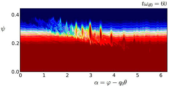
To elucidate the spatial structure of the TB formation, we have plotted in Figure 13 the mean profile of the ion pressure calculated at two different positions in $\alpha$ as a function of the poloidal flux. We see clearly there is a strong increase in the gradient of pressure near the right edge of the simulation box $\psi =1$, revealing a region (located at $\psi \sim 0.8$) where the pressure is almost constant. The observed behaviour in the ion pressure can be interpreted as a clear signature of the formation of a TB in this region where the ZF is dominant. As shown in Figure 11, electric potential fluctuations lead to the formation of a strong ZF in the region of formation of the TB. The importance of ZF lies in its ability to limit the size of interchange turbulence eddies in the poloidal flux direction and hence, effectively, to regulate turbulent transport.

In that regime, ZF has a limited impact on the saturation, implying that the dominant saturation mechanism must be of a different nature. A possible explanation is that the three-wave interaction between CTIM and the interchange turbulence ceases (like by a detuning process). Here the situation is however more complex since the wave-particle resonances lead to a Landau-type dissipation and the density and the electric potential can remain in phase in this process. The generation of ZF and its feedback to turbulence are nonlinear processes in which wave-particle interactions play a key role. In particular we have also observed the formation and propagation of trapping structures (with now particles trapped in the electric potential) as a result of the Landau damping in the nonlinear regime. Figure 14 shows a representation of the ion distribution function (obtained for a population of deeply trapped (banana) orbits for $\kappa =0$, in the bulk of the distribution).

6. Conclusions

We have performed a thorough study of the changes in the nature of the zonal flows induced by parametric three-wave process with trapped particle modes in presence of a polarisation source that allows the generation of a shear flow. We have identified a nonlinear coupling mechanism of zonal flow with trapped particles modes mediated by resonant parametric decay. Such a mechanism was possible due to the modification of the zonal flow which may now oscillates at finite frequency and enters in resonance with trapped modes leading to strong amplification. Applications of the model to the formation of transport barriers have been analized in detail.

Semi-Lagrangian simulations have been carried out, which have led to a progress in understanding the physics of low frequency zonal frequency. However, the investigation of the coupling between CTEM with the interchange turbulence and the associated wave-particle resonances has just start and the result obtained evidence that the dynamics of zonal flow seems somewhat different from that of zero frequency zonal flows induced by the Reynolds stress. Further development is still need in the area of multiscale turbulence and the low-frequency physics associated with circulating particles. Existing models for the flow shear suppression or amplification of the (interchange) turbulence and for the zonal or low-frequency GAM flow paradigm help to an overall understanding. Great effort should now be placed on the development of fast gyrokinetic modelling including both trapped and circulating particle populations, which be able to follow both the dynamics of particles and their low-frequency resonant wave-particle interactions over long times.

References

1. Diamond, P.H.; Hahm, T.S. On the dynamics of turbulent transport near marginal stability. Phys. Plasmas 1995, 2, 3640. [Google Scholar] [CrossRef]
2. Horton, W. Drift wave and transport. Rev. Modern Phys. 1999, 71, 735. [Google Scholar] [CrossRef]
3. Horton, W.; Ichikawa, Y.H. Chaos and Structures in Nonlinear Plasmas; World Scientific Publishing: Singapore; London, UK; New York, NY, USA, 1996. [Google Scholar]
4. Garbet, X. Turbulence in fusion plasmas: Key issues and impact on transport modelling. Plasma Phys. Control. Fusion 2001, 43, 1251. [Google Scholar] [CrossRef]
5. Guzdar, P.N.; Kleva, R.G.; Das, A.; Kaw, P.K. Zonal Flow and zonal magnetic field generation by finite β drift waves: A theory for low to high transitions in tokamaks. Phys. Rev. Lett. 2001, 87, 015001. [Google Scholar] [CrossRef] [PubMed]
6. Guzdar, P.N.; Kleva, R.G.; Das, A.; Kaw, P.K. Zonal Flow and field generation by finite beta drift waves and kinetic drift-Alfven waves. Phys. Plasmas 2001, 8, 3907. [Google Scholar] [CrossRef]
7. Kim, E.; Diamond, P.H. Zonal flows and transient dynamics of the LH transition. Phys. Rev. Lett. 2003, 90, 185006. [Google Scholar] [CrossRef]
8. Malkov, M.A.; Diamond, P.H.; Rosenbluth, M. On the nature of bursting in transport and turbulence in drift wave-zonal flow system. Phys. Plasmas 2001, 8, 5073. [Google Scholar] [CrossRef]
9. Malkov, M.A.; Diamond, P.H. Analytic theory of LH transition, barrier structure and hysteresis for a simple model of coupled particle and heat fluxes. Phys. Plasmas 2008, 15, 122301. [Google Scholar] [CrossRef]
10. Itoh, K.; Itoh, S.I.; Diamond, P.H.; Hahm, T.S.; Fujisawa, A.; Tynan, G.R.; Yagi, M.; Nagashima, Y. Physics of zonal flows. Phys. Plasmas 2006, 13, 055502. [Google Scholar] [CrossRef] [Green Version]
11. Zhang, Y.Z.; Liu, Z.Y.; Xie, T.; Mahajan, S.M.; Liu, J. A theory of self-organized zonal flow with fine radial structure in tokamaks. Phys. Plasmas 2017, 24, 122304. [Google Scholar] [CrossRef]
12. Ghizzo, A.; Palermo, F. Shear-flow trapped-ion-mode interaction revisited I. Influence of low-frequency zonal flow on ion-temperature-gradient driven turbulence. Phys. Plasmas 2015, 22, 082303. [Google Scholar] [CrossRef]
13. Ghizzo, A.; Palermo, F. Shear-flow trapped-ion-mode interaction revisited II. Intermittent transport associated with low-frequency zonal flow dynamics. Phys. Plasmas 2015, 22, 082304. [Google Scholar] [CrossRef]
14. Berk, H.L.; Boswell, C.J.; Borba, D.; Figueiredo, A.C.A.; Johnson, T.; Nave, M.F.F.; Pinches, S.D.; Sharapov, S.E. JET EFDA Contributors, Explanation of the JET n=0 chirping mode. Nucl. Fusion 2006, 46, S888. [Google Scholar] [CrossRef]
15. Ghizzo, A.; del Sarto, D.; Garbet, X.; Sarazin, Y. Streamer-induced transport in the presence of trapped ion modes in tokamak plasmas. Phys. Plasmas 2010, 17, 092501. [Google Scholar] [CrossRef] [Green Version]
16. Ghizzo, A.; del Sarto, D.; Palermo, F.; Biancalani, A. Transport Barriers associated to the resonant interaction between trapped particle modes triggered by plasma polarisation injection. Euro. Phys. Lett. 2017, 119, 15003. [Google Scholar] [CrossRef]
17. Xu, G.S.; Wan, B.N.; Wang, H.Q.; Guo, H.Y.; Zhao, H.L.; Liu, A.D.; Naulin, V.; Diamond, P.H.; Tynan, G.R.; Xu, M.; et al. First evidence of the role of zonal flows for the L.H. transition at marginal imput power in the EAST tokamak. Phys. Rev. Lett. 2011, 107, 125001. [Google Scholar] [CrossRef]
18. Winsor, N.; Johnson, J.L.; Dawson, J.M. Geodesic AcousticWaves in Hydromagnetic systems. Phys. Fluids 1968, 11, 2448. [Google Scholar] [CrossRef]
19. Scott, B. The geodesic transfer effect on zonal flows in tokamak edge turbulence. Phys. Lett. A 2003, 320, 53–62. [Google Scholar] [CrossRef] [Green Version]
20. Conway, G.D.; Angioni, C.; Ryter, F.; Sauter, P.; Vicente, J. ASDEX Upgrade Team, Mean and oscillating plasma flows and turbulence interactions accross the L-H confinement transition. Phys. Rev. Lett. 2011, 106, 065001. [Google Scholar] [CrossRef]
21. Coda, S.; Porkolab, M.; Burrell, K.H. Signature of turbulent zonal flows observed in the DIII-D tokamak. Phys. Rev. Lett. 2001, 86, 4835–4838. [Google Scholar] [CrossRef]
22. Watari, T.; Hamada, Y.; Notake, T.; Takeuchi, N.; Itoh, K. Geodesic acoustic mode oscillation in low frequency range. Phys. Plasmas 2006, 13, 062504. [Google Scholar] [CrossRef]
23. Xu, G.S.; Naulin, V.; Fundamenski, W.; Hidalgo, C.; Alonso, J.A.; Silva, C.; Gonzalves, B.; Nielsen, A.H.; Rasmussen, J.J.; Krasheninnikov, S.I.; et al. Stamp and JET EFDA Contributors, Blob-Hole formation and zonal-flow generation in the edge plasma of the JET tokamak. Nucl. Fusion 2009, 49, 092002. [Google Scholar] [CrossRef]
24. Robinson, P.A. Nonlinear wave collapse and strong turbulence. Rev. Modern Phys. 1997, 69, 507. [Google Scholar] [CrossRef]
25. Rajaraman, R. Solitons and Instantons, An Introduction to Solitons and Instantons in Quantum Field Theory; Elsevier Science, Publishers B.V.: North-Holland, The Amsterdam, 1989. [Google Scholar]
26. Depret, G.; Garbet, X.; Bertrand, P.; Ghizzo, A. Trapped-ion driven turbulence in tokamak plasmas. Plasma Phys. Control. Fusion 2000, 42, 949. [Google Scholar] [CrossRef]
27. Drouot, T.; Gravier, E.; Reveille, T.; Ghizzo, A.; Bertrand, P.; Garbet, X.; Sarazin, Y.; Cartier-Michaud, T. A gyro-kinetic model for trapped electron and ion modes. Eur. Phys. J. D 2014, 68, 280. [Google Scholar] [CrossRef]
28. Drouot, T.; Gravier, E.; Reveille, T.; Sarrat, M.; Collard, M.; Bertrand, P.; Ghendrih, P.; Sarazin, Y.; Garbet, X. Global gyrokinetic simulations of trapped-electron mode and trapped-ion mode microturbulence. Phys. Plasmas 2015, 22, 082302. [Google Scholar] [CrossRef]
29. Gravier, E.; Lesur, M.; Reveille, T.; Drouot, T. Stimulated zonal flow generation in the case of TEM and TIM. Phys. Plasmas 2016, 23, 092507. [Google Scholar] [CrossRef]
30. Palermo, F.; Garbet, X.; Ghizzo, A.; Cartier-Michaud, T.; Ghendrih, P.; Grandgirard, V.; Sarazin, Y. Shear flow instabilities induced by trapped ion modes in collisionless temperature gradient turbulence. Phys. Plasmas 2015, 22, 042304. [Google Scholar] [CrossRef]
31. Fong, B.H.; Hahm, T.S. Bounce-averaged kinetic equations and neoclassical polarization density. Phys. Plasmas 1999, 6, 188. [Google Scholar] [CrossRef]
32. Wang, L.; Hahm, T.S. Nonlinear gyrokinetic theory with polarisation drift. Phys. Plasmas 2010, 17, 082304. [Google Scholar] [CrossRef]
33. Kadomtsev, B.B.; Pogutse, O.P. Trapped particles in toroidal magnetic systems. Nucl. Fusion 1971, 11, 67. [Google Scholar] [CrossRef]
34. Kadomtsev, B.B.; Pogutse, O.P. Review of Plasma Physics; Leontovich, M., Ed.; Consultants Bureau: New York, NY, USA, 1970; Volume 5. [Google Scholar]
35. del Sarto, D.; Ghizzo, A. Hasegawa-Wakatani and modified Hasegawa-Wakatani turbulence induced by ion-temperature-gradient instabilities. Fluids 2017, 2, 65. [Google Scholar] [CrossRef]
36. Dif-Pradalier, G.; Hornung, G.; Ghendrih, P.; Sarazin, Y.; Clairet, F.; Vermare, L.; Diamond, P.H.; Abiteboul, J.; Cartier-Michaud, T.; Ehrlacher, C.; et al. Finding the elusive E × B staircase in magnetized plasmas. Phys. Rev. Lett. 2015, 114, 085004. [Google Scholar] [CrossRef]
37. Dif-Pradalier, G.; Hornung, G.; Garbet, X.; Ghendrih, P.; Grandgirard, V.; Latu, G.; Sarazin, Y. The E × B staircase of magnetized plasmas. Nucl. Fusion 2017, 57, 066026. [Google Scholar] [CrossRef]
38. Brizard, A. Beyond linear gyrocenter polarization in gyrokinetic theory. Plasma Phys. 2013, 20, 092309. [Google Scholar] [CrossRef] [Green Version]
39. Strugarek, A.; Sarazin, Y.; Zarzoso, D.; Abiteboul, J.; Brun, A.S.; Michaud, T.C.; Pradalier, G.D.; Garbet, X.; Ghendrih, P.H.; Grangirard, V.; et al. Unraveling Quasiperiodic relaxations of transport barriers with gyrokinetic simulations of tokamak plasmas. Phys. Rev. Lett. 2013, 111, 145001. [Google Scholar] [CrossRef] [PubMed]
40. Tang, W.M.; Rutherford, P.H.; Furth, H.P.; Adam, J.C. Stabilization of trapped-particle modes by reversed-gradient profiles. Phys. Rev. Lett. 1975, 35, 660. [Google Scholar] [CrossRef]
41. Tang, W.M. Effect of toroidal gradient drifts on the dissipative trapped-ion instability. Phys. Fluids 1974, 17, 1249. [Google Scholar] [CrossRef]
42. Marchand, R.; Tang, W.M.; Rewoldt, G. Two-dimensional analysis of trapped-ion eigenmodes. Phys. Plasmas 1995, 2, 3384. [Google Scholar]
43. LaQuey, R.E.; Mahajan, S.M.; Rutherford, P.H.; Tang, W.M. Nonlinear saturation of the trapped-ion mode. Phys. Rev. Lett. 1975, 34, 391. [Google Scholar] [CrossRef]
44. Nishimura, S. Interchange mode excited by trapped energetic ions. Phys. Plasmas 2015, 22, 072505. [Google Scholar] [CrossRef]
45. Qiu, Z.; Chen, L.; Zonca, F. Kinetic theory of geodesic acoustic modes in toroidal plasmas: A brief review. Plasma Sci. Technol. 2018, 20, 094004. [Google Scholar] [CrossRef]
Figure 1. Plot of the mean electric potential ϕ α (in solid line) and its first derivative d ϕ α d ψ (in dotted line) as a function of the poloidal flux ψ . The curves show the behaviour of these quantities from solutions given by Equations (23) and (24) when polarisation injection is taken into account in the initial data.
Plasma 02 00017 g001
Figure 2. Plot of the quantity g 0 E , ψ = 0.5 e E T 0 as a function of the energy E / T 0 for different values of the parameter β which determines the level of polarisation injection.
Plasma 02 00017 g002
Figure 3. Emergence of a blob-hole pattern in both potential ϕ (on top panel) and the first moment of the distribution g i (shown in middle panel) at time t ω d 0 = 4.6 . We see clearly the formation of a hole in the electric potential in which non linear coherent vortices are formed. Notice that such structure are very similar to quasi-regular patters referred as E × B staircases formed of turbulent regions interspersed with narrow confining micro-barriers. Mean averaged quantities on the poloidal flux are plotted on bottom panels.
Plasma 02 00017 g003
Figure 4. The corresponding representation of the first moment of the distribution g i at time t ω d 0 = 9.6 . We see clearly that the stabilization of the system is directly linked to the decrease in size of the turbulent region.
Plasma 02 00017 g004
Figure 5. Time evolution of the energy of the zonal flow E Z F on the top panel together with and the corresponding turbulent energy E t u r b on the middle panel well inside in the regime of the interchange turbulence. The two first bursts observed in the turbulent activity in the middle panel for t ω d 0 80 , precedes that of the zonal flow energy. Such a behaviour points out the ZF is driven by the drift-wave turbulence through the Reynolds tensor, as expected in this type of scenario. The situation is somewhat different after time t ω d 0 80 when resonant processes take place. An intermittent behaviour is now observed with the emergence of strong narrow peaks produced at the same time for both ZF and turbulence as shown on bottom panel where a zoom is plotted.
Plasma 02 00017 g005
Figure 6. Phase space ψ , α representation of the electric potential at three different times during the plasma evolution. On top panel the formation and growth of linear streamers made the mode n = 10 , followed by the stretching of structures on middle panel. The bottom panel shows the excitation and growth of non linear streamers during the turbulent burst.
Plasma 02 00017 g006
Figure 7. Dynamics behaviour of the E × B shear flow velocity, in the first phase of the interaction. On top and middle panels the electric potential exhibits a soliton-type structure characterized by the emergence of a strong narrow peak which indicates the excitation of a shear flow and the formation of a forward propagating solution. On bottom panels the corresponding representation of the mean potential ϕ ψ . We observe clearly the emergence of a strong peak located at α 3 . at the leftside panel propagating in α during the field amplification.
Plasma 02 00017 g007
Figure 8. Dynamical behaviour of the electric potential in the second phase of the interaction when the resonant three-wave parametric process takes place. On top panel when the peak is reached in amplitude, and on bottom panel when the turbulence level is weak.
Plasma 02 00017 g008
Figure 9. The instability disappears completely without polarisation source (when β = 0 ). We have plotted here the time evolution of the different energies: the ion kinetic energy E k i n , i (on top panel), the zonal flow energy E Z F which remains strictly to zero (on middle panel) and finally the fluctuating turbulent energy E t u r b (on bottom panel) which remains at a very small level.
Plasma 02 00017 g009
Figure 10. Time evolution of the energies of the different actors implicated in the interaction: the ion kinetic energy for CTIM on top panel, together with the turbulence (in blue) and ZF (in red color) plotted on the same curve on bottom panel. A first burst of turbulence can be observed at time t ω d 0 55 which is connected to the growth of the (interchange) turbulence. The ZF is then impacted by the emergence of streamers. Two second peaks are formed very rapidly followed by a slow increase of the ZF and the suppression of the turbulence: the system is then dominated by the ZF and the emergence of a TB.
Plasma 02 00017 g010
Figure 11. Phase space representation of the electric potential at three different times during the formation of the TB. The system allows a key role played by streamers in the intermittent regime with the emergence of n = 30 streamers on the middle panel. The importance of ZF lies in its ability to limit the (radial) size of interchange turbulence eddies and hence, effectively, to regulate turbulent transport (on bottom panel).
Plasma 02 00017 g011
Figure 12. Continuing the presentation of results shown in Figure 10 and Figure 11, the corresponding behaviour of the ion pressure taken at the same instants: we observe the suppression of turbulence in the region of the TB located around ψ 0.8 .
Plasma 02 00017 g012
Figure 13. Plot of the mean profile of the ion pressure calculated at two different positions in α (shown here by two different colors) as a function of the poloidal flux. We see clearly that a strong increase in the gradient of pressure near the right edge of the simulation box ψ = 1 , revealing a region of the TB formation (located at ψ 0.8 ) where the pressure is almost constant.
Plasma 02 00017 g013
Figure 14. Phase space presentation of the ion distribution function obtained for a population of deeply banana orbits for κ = 0 , in the bulk of the distribution. The generation of ZF and its feedback to turbulence are nonlinear processes in which wave-particle interactions play a key role. In particular such wave-particle resonances lead to a Landau-type dissipation mechanism, with the emergence of trapping structures in the electric potential.
Plasma 02 00017 g014