

Machine Learning Based Predictive Modeling of Electrical Discharge Machining of Cryo-Treated NiTi, NiCu and BeCu Alloys
 ,
,  ,
,  ,
,
Abstract
:
1. Introduction
2. Understanding Supervised Machine Learning Algorithms
3. Materials and Methods
4. Results
5. Discussion
6. Conclusions
Author Contributions
Funding
Data Availability Statement
Acknowledgments
Conflicts of Interest
References
- Ming, W.; Zhang, S.; Zhang, G.; Du, J.; Ma, J.; He, W.; Cao, C.; Liu, K. Progress in modeling of electrical discharge machining process. Int. J. Heat Mass Transf. 2022, 187, 122563. [Google Scholar] [CrossRef]
- Shastri, R.K.; Mohanty, C.P.; Dash, S.; Gopal, K.M.P.; Annamalai, A.R.; Jen, C.P. Reviewing Performance Measures of the Die-Sinking Electrical Discharge Machining Process: Challenges and Future Scopes. Nanomaterials 2022, 12, 384. [Google Scholar] [CrossRef]
- Boopathi, S. An extensive review on sustainable developments of dry and near-dry electrical discharge machining processes. J. Manuf. Sci. Eng. 2022, 144, 050801. [Google Scholar] [CrossRef]
- Baroi, B.K.; Patowari, P.K. A review on sustainability, health, and safety issues of electrical discharge machining. J. Braz. Soc. Mech. Sci. Eng. 2022, 44, 59. [Google Scholar] [CrossRef]
- Kannan, E.; Trabelsi, Y.; Boopathi, S.; Alagesan, S. Influences of Cryogenically Treated Work Material on Near-Dry Wire-Cut Electrical Discharge Machining Process. Surf. Topogr. Metrol. Prop. 2022, 10, 015027. Available online: https://iopscience.iop.org/article/10.1088/2051-672X/ac53e1 (accessed on 12 July 2022). [CrossRef]
- Chaudhari, R.; Prajapati, P.; Khanna, S.; Vora, J.; Patel, V.K.; Pimenov, D.Y.; Giasin, K. Multi-response optimization of Al2O3 nanopowder-mixed wire electrical discharge machining process parameters of nitinol shape memory alloy. Materials 2022, 15, 2018. [Google Scholar] [CrossRef]
- Karthik Pandiyan, G.; Prabaharan, T.; Jafrey Daniel James, D.; Sivalingam, V. Machinability analysis and optimization of electrical discharge machining in AA6061-T6/15wt.% SiC composite by the multi-criteria decision-making approach. J. Mater. Eng. Perfor. 2022, 31, 3741–3752. [Google Scholar] [CrossRef]
- Vora, J.; Khanna, S.; Chaudhari, R.; Patel, V.K.; Paneliya, S.; Pimenov, D.Y.; Giasin, K.; Prakash, C. Machining parameter optimization and experimental investigations of nano-graphene mixed electrical discharge machining of nitinol shape memory alloy. J. Mater. Res. Technol. 2022, 19, 653–668. [Google Scholar] [CrossRef]
- Akıncıoğlu, S. Taguchi optimization of multiple performance characteristics in the electrical discharge machining of the TiGr2. Facta Univ. Mech. Eng. 2022, 20, 237–253. [Google Scholar] [CrossRef]
- Danish, M.; Al-Amin, M.; Abdul-Rani, A.M.; Rubaiee, S.; Ahmed, A.; Zohura, F.T.; Ahmed, R.; Yildirim, M.B. Optimization of hydroxyapatite powder mixed electric discharge machining process to improve modified surface features of 316L stainless steel. Proc. Inst. Mech. Eng. Part E J. Process Mech. Eng. 2022. [Google Scholar] [CrossRef]
- Kam, M.; İpekçi, A.; Argun, K. Experimental investigation and optimization of machining parameters of deep cryogenically treated and tempered steels in electrical discharge machining process. Proc. Inst. Mech. Eng. Part E J. Process Mech. Eng. 2022, 236, 1927–1935. [Google Scholar] [CrossRef]
- Gautam, N.; Goyal, A.; Sharma, S.S.; Oza, A.D.; Kumar, R. Study of various optimization techniques for electric discharge machining and electrochemical machining processes. Mater. Today Proc. 2022, 57, 615–621. [Google Scholar] [CrossRef]
- Shukla, S.K.; Priyadarshini, A. Application of machine learning techniques for multi objective optimization of response variables in wire cut electro discharge machining operation. Mater. Sci. For. 2019, 969, 800–806. [Google Scholar] [CrossRef]
- Ghosh, I.; Sanyal, M.K.; Jana, R.K.; Dan, P.K. Machine learning for predictive modeling in management of operations of EDM equipment product. In Proceedings of the Second International Conference on Research in Computational Intelligence and Communication Networks (ICRCICN), Kolkata, India, 23–25 September 2016; pp. 169–174. [Google Scholar] [CrossRef]
- Ulas, M.; Aydur, O.; Gurgenc, T.; Ozel, C. Surface roughness prediction of machined aluminum alloy with wire electrical discharge machining by different machine learning algorithms. J. Mater. Res. Tech. 2020, 9, 12512–12524. [Google Scholar] [CrossRef]
- Ali, M.A.; Samsul, M.; Hussein, N.I.S.; Rizal, M.; Izamshah, R.; Hadzley, M.; Kasim, M.S.; Sulaiman, M.A.; Sivarao, S. The Effect of Edm Die-sinking Parameters on Material Removal Rate of Beryllium Copper Using Full Factorial Method. Middle-East J. Sci. Res. 2013, 16, 44–50. [Google Scholar] [CrossRef]
- Selvakumar, G.; Sarkar, S.; Modern, S.M.I.J. Experimental analysis on WEDM of monel 400 alloys in a range of thicknesses. Int. J. Mod. Manuf. Technol. 2012, 4, 113–120. [Google Scholar]
- Kumar, V.; Kumar, V.; Kumar, K. An experimental analysis and optimization of machining rate and surface characteristics in WEDM of Monel-400 using RSM and desirability approach. J. Ind. Eng. Int. 2015, 11, 297–307. [Google Scholar] [CrossRef]
- Kumar, N.E.A.; Babu, A.S. Influence of input parameters on the near-dry WEDM of Monel alloy. Mater. Manuf. Process. 2018, 33, 85–92. [Google Scholar] [CrossRef]
- Daneshmand, S.; Kahrizi, E.F.; Abedi, E.; Abdolhosseini, M.M. Influence of machining parameters on electro discharge machining of NiTi shape memory alloys. Int. J. Electrochem. Sci. 2013, 8, 3095–3104. [Google Scholar]
- Gangele, A.; Mishra, A. Surface roughness optimization during machining of NiTi shape memory alloy by EDM through Taguchi’s technique. Mater. Today Proc. 2020, 29, 343–347. [Google Scholar] [CrossRef]
- Daneshmand, S.; Monfared, V.; Neyestanak, A.A.L. Effect of tool rotational and Al2O3 powder in electro discharge machining characteristics of NiTi-60 shape memory alloy. Silicon 2016, 9, 273–283. [Google Scholar] [CrossRef]
- Pogrebnjak, A.D.; Bratushka, S.N.; Beresnev, V.M.; Levintant-Zayonts, N. Shape memory effect and superelasticity of titanium nickelide alloys implanted with high ion doses. Russ. Chem. Rev. 2013, 82, 1135–1159. [Google Scholar] [CrossRef]


| Properties | NiTi Alloy | NiCu Alloy | BeCu Alloy | Copper Electrode | ||||
|---|---|---|---|---|---|---|---|---|
| Untreated | Treated | Untreated | Treated | Untreated | Treated | Untreated | Treated | |
| Thermal conductivity (k), W/mk | 10 | 12.9 | 21.8 | 22.2 | 130 | 135.9 | 391.1 | |
| Electrical conductivity (σ), S/mm | 3.268 | 4.219 | 5.515 | 5.625 | 5.645 | 5.902 | 10 | 26.316 |
| Workpiece Name and Treatment | Workpiece Electrical Conductivity (S/m) | Gap Current (A) | Gap Voltage (V) | Pulse On Time (μs) | Pulse Off Time (μs) | Material Removal Rate (mm3/min) |
|---|---|---|---|---|---|---|
| NiTi Untreated | 3268 | 8 | 40 | 13 | 5 | 2.09 |
| NiTi Untreated | 3268 | 12 | 55 | 26 | 7 | 4.56 |
| NiTi Untreated | 3268 | 16 | 70 | 38 | 9 | 7.11 |
| NiTi Treated | 4219 | 8 | 40 | 26 | 7 | 3.96 |
| NiTi Treated | 4219 | 12 | 55 | 38 | 9 | 6.5 |
| NiTi Treated | 4219 | 16 | 70 | 13 | 5 | 4.16 |
| NiCu Untreated | 5515 | 8 | 55 | 13 | 9 | 2.76 |
| NiCu Untreated | 5515 | 12 | 70 | 26 | 5 | 3.33 |
| NiCu Untreated | 5515 | 16 | 40 | 38 | 7 | 9 |
| NiCu Treated | 5625 | 8 | 70 | 38 | 7 | 3.1 |
| NiCu Treated | 5625 | 12 | 40 | 13 | 9 | 5.98 |
| NiCu Treated | 5625 | 16 | 55 | 26 | 5 | 6.26 |
| BeCu Untreated | 5645 | 8 | 55 | 38 | 5 | 3.41 |
| BeCu Untreated | 5645 | 12 | 70 | 13 | 7 | 3.08 |
| BeCu Untreated | 5645 | 16 | 40 | 26 | 9 | 9.08 |
| BeCu Treated | 5902 | 8 | 70 | 26 | 9 | 2.8 |
| BeCu Treated | 5902 | 12 | 40 | 38 | 5 | 6.7 |
| BeCu Treated | 5902 | 16 | 55 | 13 | 7 | 6.03 |
| Algorithms | Mean Square Error | Mean Absolute Error | R2 |
|---|---|---|---|
| Random Forest | 0.745 | 0.764 | 0.856 |
| Decision Tree | 0.965 | 0.792 | 0.814 |
| Gradient Boosting | 0.360 | 0.529 | 0.930 |
| Artificial Neural Network | 0.255 | 0.098 | 0.749 |
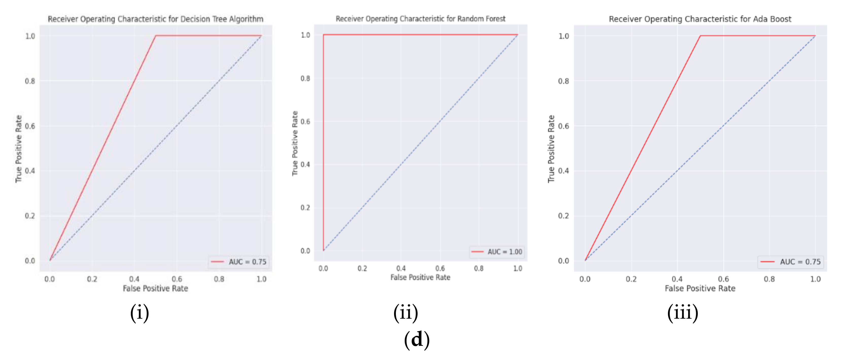
| Algorithms | Precision Value of ‘0’ | Precision Value of ‘1’ | Recall Value of ‘0’ | Recall Value of ‘1’ | Overall F1-Score |
|---|---|---|---|---|---|
| Decision Tree | 1.00 | 0.67 | 0.50 | 1.00 | 0.75 |
| Random Forest | 1.00 | 1.00 | 1.00 | 1.00 | 1.00 |
| AdaBoost | 1.00 | 0.67 | 0.50 | 1.00 | 0.75 |
Publisher’s Note: MDPI stays neutral with regard to jurisdictional claims in published maps and institutional affiliations. |
© 2022 by the authors. Licensee MDPI, Basel, Switzerland. This article is an open access article distributed under the terms and conditions of the Creative Commons Attribution (CC BY) license (https://creativecommons.org/licenses/by/4.0/).
Share and Cite
Jatti, V.S.; Dhabale, R.B.; Mishra, A.; Khedkar, N.K.; Jatti, V.S.; Jatti, A.V. Machine Learning Based Predictive Modeling of Electrical Discharge Machining of Cryo-Treated NiTi, NiCu and BeCu Alloys. Appl. Syst. Innov. 2022, 5, 107. https://doi.org/10.3390/asi5060107
Jatti VS, Dhabale RB, Mishra A, Khedkar NK, Jatti VS, Jatti AV. Machine Learning Based Predictive Modeling of Electrical Discharge Machining of Cryo-Treated NiTi, NiCu and BeCu Alloys. Applied System Innovation. 2022; 5(6):107. https://doi.org/10.3390/asi5060107
Chicago/Turabian StyleJatti, Vijaykumar S., Rahul B. Dhabale, Akshansh Mishra, Nitin K. Khedkar, Vinaykumar S. Jatti, and Ashwini V. Jatti. 2022. "Machine Learning Based Predictive Modeling of Electrical Discharge Machining of Cryo-Treated NiTi, NiCu and BeCu Alloys" Applied System Innovation 5, no. 6: 107. https://doi.org/10.3390/asi5060107