LOVE Is in the R—Two R Tools for Local Vegetation Reconstruction

Abstract

Pollen deposition in small lakes and peatlands is composed of local pollen deposition arriving from the nearby vegetation and of regional pollen deposition arriving from farther away. The LOVE model aims to reconstruct past vegetation on a small local scale by extracting only the local pollen signal. To this end, pollen deposition from small sites is related to pollen deposition from large lakes with predominantly regional pollen deposition. We here present a new implementation of the LOVE model in the R environment for statistical computing that is more user friendly than existing implementations. It allows more readily application with fossil pollen data and facilitates extensive testing of the approach in simulated landscapes. The LOVE model derives from critical mathematical assumptions that strongly limit its application. We additionally present LOVEoptim as an adjusted approach to local-scale reconstructions. Other than in LOVE, past local plant abundances are approximated using numerical optimization. Tests in a simulated landscape, which is based on true landscape patterns from digital maps, show that both approaches are valid. Due to fewer mathematical assumptions, LOVEoptim is more widely applicable. The modeling results help to better interpret the spatial scale of vegetation reflected in LOVE/LOVEoptim reconstructions.

1. Introduction

Pollen deposition in small basins, such as forest hollows, includes a large proportion of extra-local pollen deposition from the nearby vegetation, which renders pollen records from such sites useful for the reconstruction of past vegetation at a local scale [1,2]. Pollen deposition in such sites, however, also includes regional pollen deposition arriving from farther away, which obscures the local pollen signal. Reconstructing the local vegetation composition therefore requires the extraction of the local component from the total pollen assemblage. So far, two approaches for local-scale reconstructions with pollen data from small sites have been developed—LOVE [3] and Marco Polo [4]. Both approaches produce local-scale reconstructions by relating pollen counts from small sites to pollen counts from a nearby large lake with predominately regional pollen deposition. In LOVE, reconstructions are produced using an analytical model. In Marco Polo, reconstructions are produced by iterative manipulations of the pollen sum. Tests with surface pollen samples from small forest hollows suggest that both approaches perform reasonably well [4].

For application of the LOVE model, Shinya Sugita developed a command-line C program. The first goal of the present study is to introduce a more user-friendly and flexible implementation of the LOVE model in the R environment for statistical computing [5]. Moreover, the LOVE model is based on two critical mathematical assumptions that limit its application to very specific landscape settings and studies with numerous small sample sites (see Section 2.1). Here, we propose an alternative approach that avoids these assumptions. Like LOVE, it derives from the fundamental assumption that the total pollen deposition of each taxon at a sample site is the sum of its local and its regional pollen deposition. Different from LOVE, the local vegetation is not estimated by a single analytical model, but is approximated using numerical optimization. In the following paper, we introduce and test the approach.

For the tests, we have developed an R tool that produces a series of landscape scenarios from digital maps and from that it simulates pollen deposition in user-defined sample sites. Using this model, we test three software tools for local-scale reconstructions: the command-line LOVE program as well as the R tools ‘LOVEr’ and ‘LOVEoptim’. For our study region, we selected the Dobbin area, in north-eastern Germany, which is subject to ongoing palynological research in small and large basins as well as to archaeological research within the Collaborative Research Centre CRC1266 “Scales of Transformation-Human-Environmental Interaction in Prehistoric and Archaic Societies” [6].

2. Materials and Methods

2.1. The Theory of Our Approach

The LOVE model [3] is based on fundamental theories about the pollen representation of vegetation in lakes and peatlands by [7,8]. The theory predicts that the total pollen deposition at a small depositional basin is the sum of the local pollen deposition coming from the vicinity of the study site, and the regional pollen deposition coming from farther away. Stand-scale reconstructions first require extraction of the local component from the total pollen deposition and then to translate the local pollen deposition into local vegetation composition. Extracting the local component is straightforward if pollen accumulation rates (PARs) are available; it can simply be calculated for each species as the PARs in the small site minus the PARs in the large site. More commonly, only pollen percentage data are available and extracting the local component is more complicated. The LOVE model uses two critical mathematical assumptions to produce an analytical solution to this problem, i.e., a single equation to calculate the local vegetation composition directly. The model was originally set up to work with multiple small study sites. The first assumption is that ‘the total sum of distance-weighted plant abundance of all taxa within the relevant source area of pollen at site k, is similar among study sites’ [3]. Distance weighting is determined by the pollen dispersal pattern, which itself is determined by, e.g., the fall speed and hence the size of pollen. In reality, the abundances of taxa with large and small pollen grains may well differ between sample sites, and so the total distance-weighted plant abundance will differ as well. The second assumption is that ‘vegetation within the relevant source area is homogeneous and its composition is the same as the regional vegetation composition’. This assumption contradicts the very idea of the LOVE model that local vegetation composition is different from regional vegetation composition. The assumption can possibly be meaningful when looking at the average vegetation composition of a set of small sample sites, but not for a single site. Yet, even for a set of sample sites, the overall average local vegetation composition will likely differ from the regional vegetation composition. In the study region of northern Germany, for example, the vegetation in the vicinity of small lakes and peatlands is usually quite different from the vegetation farther away. Overall, both assumptions appear to limit the application of the LOVE model to peculiar landscape and vegetation settings. Note that both assumptions are necessary to arrive at an analytical mathematical solution to the problem.

In our alternative numerical approach, local vegetation composition is not calculated directly but approximated by optimization. Like LOVE, our implementation is based on the fundamental assumption that the total pollen deposition in a small sample site is the sum of the local and the regional pollen deposition. The local vegetation composition is approximated in three main steps. In the first step, regional vegetation composition is calculated using a pollen record from a nearby large lake and the REVEALS model [9]. In the second step, regional pollen deposition for the small sample site is calculated by multiplying the regional abundance of each taxon with the respective pollen productivity estimate and a distance-weighting factor. The third step is iterative. It starts from random estimates of local vegetation composition. From that, local pollen deposition is calculated by multiplying the (initially random) local plant abundances with the corresponding pollen productivity estimates and distance-weighting factors. The sum of local and regional pollen deposition, i.e., the total pollen deposition, can be expressed as pollen composition and compared to the composition of true pollen samples from the sample site. Using numerical optimization, the local vegetation composition is then adjusted until the resulting, modeled pollen composition has converged with the true pollen composition at the sample site. We name our approach LOVEoptim because it derives from the same principle as the LOVE model, but uses numerical optimization to estimate the local vegetation composition.

2.2. R Implementation of LOVE (LOVEr)

For more readily application of the LOVE model, we have implemented it in the R environment for statistical computing [5], as the ‘LOVEr’ function within the ‘disqover’ R package (https://disqover.botanik.uni-greifswald.de/ (accessed on 23 February 2024)). LOVEr is based on Equations (6) and (7) of from the LOVE model [3], with three small adaptations. Pollen dispersal factors are calculated using the ‘DispersalFactorK’ function from the ‘disqover’ R package. Regional vegetation estimates are calculated with the ‘REVEALSinR’ function, also from the ‘disqover’ R package. Finally, error estimates are produced by repeated model runs, with random noise added in the regional and local pollen counts and in the pollen productivity estimates during each run.

2.3. R Implementation of LOVEoptim

LOVEoptim is also implemented as function in the ‘disqover’ R package, and uses several existing functions from the package. Regional vegetation composition (step 1) is calculated using the ‘REVEALSinR’ function. Regional pollen deposition for small sites (step 2) is then calculated by multiplying the regional abundance of each pollen taxon with the corresponding pollen productivity estimate and distance-weighting factor. The latter are calculated with the ‘DispersalFactorK’ function. To find the most suitable local vegetation composition (step 3), the Differential Evolution Optimization method ‘DEoptim’ from the ‘RcppDE’ R package is used [10]. In this step, the best match between modeled and true pollen deposition in the small basin is sought by iteratively adjusting the local vegetation composition. The difference between modeled and true pollen composition is expressed as log-Euclidean distance.

As in LOVEr, we have chosen not to define a suitable local area a priori, such as the RSAP. Instead, the calculations are performed iteratively, increasing the area considered to be local during each step. We will later discuss the selection of the most appropriate size of the local area based on the model output. To increase the flexibility of the calculations, we do not simply calculate the local and the regional pollen deposition by summarizing all inner (local vegetation) and outer (regional vegetation) rings. Instead, pollen deposition is calculated for each individual, successively larger ring around the small site. In the first iteration, only the innermost ring is assigned as local, all others as regional. With each iteration, one additional ring is assigned as local. The vegetation composition of each ring is set to either the local or the regional vegetation composition, respectively. In other words, consecutive rings are added that are assumed to have local vegetation cover that deviates from the regional background vegetation cover. The pollen deposition of all local rings is subsumed under local pollen deposition, the pollen deposition of all regional rings under regional pollen deposition. If the coverage of major land cover classes such as lakes, peatlands and terrestrial areas is provided for each ring, e.g., from digital maps, this approach allows the basin boundary to be considered more accurately, especially in the case of non-circular basins. It is also possible to account for additional lakes or other types of non-vegetated areas in the vicinity of a sample site.

LOVEoptim can also be used for terrestrial taxa only, i.e., excluding wetland and wetland pollen taxa, at least when terrestrial and wetland pollen taxa are clearly distinguishable. Error estimates are determined in a similar way to LOVEr, i.e., by repeated calculations with random noise added to the input data, i.e., the regional and local pollen counts and pollen productivity estimates.

2.4. Model Testing

To evaluate the suitability of LOVEr as an R implementation of the LOVE model and of LOVEoptim as our new approach, we tested both in a simulated landscape setting. For comparison, the command-line LOVE software by Shinya Sugita was also included in the tests. We will refer to this tool as LOVEcmd.

The simulations and tests are also set-up in R and include three main steps:

• Create realistic vegetation scenarios: To this end, first a digital vector map of a landscape pattern is imported, in our case, the digital soil map BÜK200 (with a scale of 1:200,000, https://services.bgr.de/boden/buek200 (accessed on 16 November 2023)). The map pattern is translated into a vegetation map by assigning each map category a user-defined vegetation composition (

  Table 1. Vegetation composition assigned to each map unit in the simulations (unit 1 = lakes).

  Map Unit	Lakes	Alnus	Betula	Corylus	Fagus	Fraxinus	Pinus	Tilia	Ulmus	Grasses	Secale
  1	1	0	0	0	0	0	0	0	0	0	0
  2	0	0	0.2	0	0	0	0.75	0	0	0	0.05
  3	0	0	0.6	0	0.1	0	0.1	0.1	0	0	0.1
  4	0	0.1	0.1	0.1	0.6	0	0	0	0.1	0	0
  5	0	0.1	0	0	0	0.4	0	0	0.4	0.1	0
  6	0	0	0.1	0.1	0.1	0	0.1	0.6	0	0	0
  7	0	0	0	0.4	0	0.2	0	0.2	0	0	0.2
  8	0	0.1	0.1	0.8	0	0	0	0	0	0	0
  9	0	0	0.1	0.3	0.2	0	0	0.3	0.1	0	0
  10	0	0	0.1	0	0	0	0.1	0	0	0.8	0
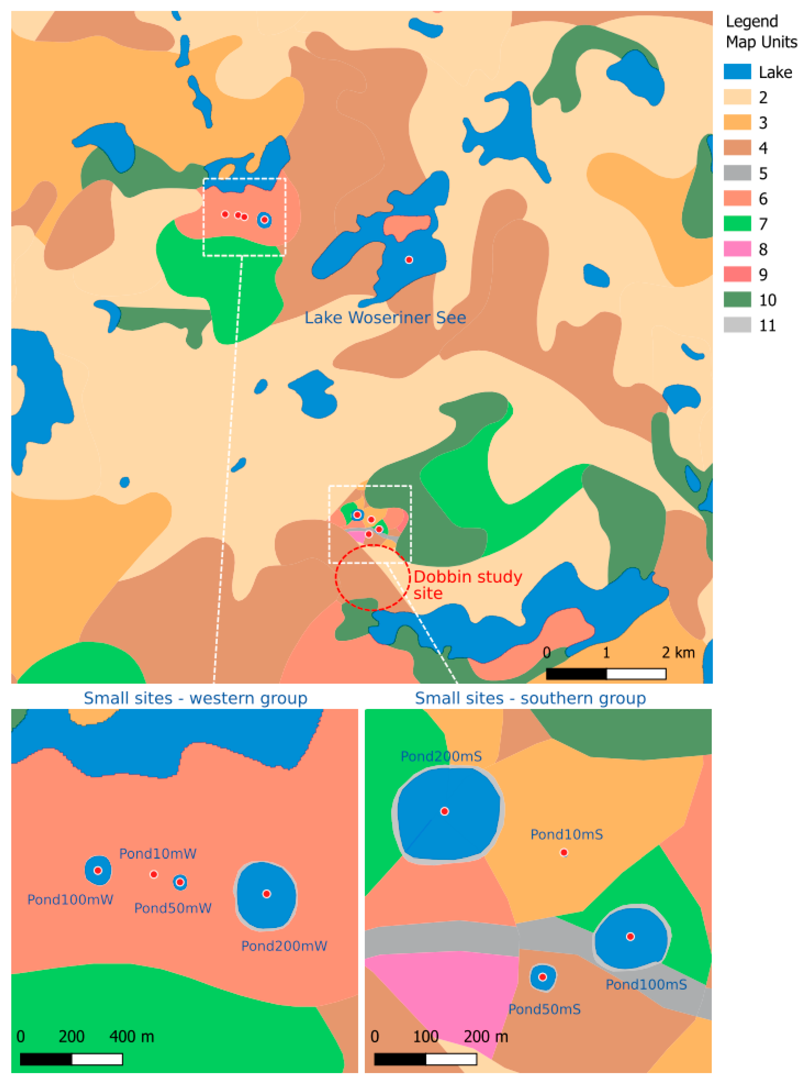
  11	0	0.5	0.25	0	0	0.25	0	0	0	0	0

  ). As study region, we selected the Dobbin area, in north-eastern Germany, which is subject to ongoing palynological research in small and large basins as well as archaeological research within the Collaborative Research Centre CRC1266 “Scales of Transformation-Human-Environmental Interaction in Prehistoric and Archaic Societies” ([6]; Figure 1). Due to its rather coarse resolution, the BÜK200 map does not show the existing small basins in the vicinity of the Dobbin site. Therefore, we added two sets of virtual small ponds with a diameter of ~10, ~50, ~100 and ~200 m into our study landscape. All sites have been drawn with a narrow surrounding buffer to mimic the often present lake shore vegetation with, e.g., alder and birch (Figure 1). As regional pollen site, we have chosen lake Woseriner See, which is also being investigated in the frame of the CRC1266 [11,12]. The small sites are located ~4.5 km south and ~3 km west of the regional site. The BÜK200 map covers the whole of Germany. In the present simulations, we consider the area with a radius of 100 km around each study site.
• Calculate pollen deposition: To calculate the pollen deposition in each study site from the resulting vegetation map, we extracted the vegetation composition around each study site for consecutive, increasingly larger rings. To arrive at the pollen deposition coming from each ring, the total area (in m²) occupied by each pollen taxon is multiplied by the corresponding pollen productivity (

  Table 2. Fall speed of pollen and relative pollen productivity estimates used in the present simulations.

  Taxon	Fall Speed	PPE	PPE SD
  Alnus	0.024	4	0.4
  Betula	0.024	4	0.4
  Corylus	0.024	3	0.3
  Fagus	0.060	1	0.1
  Fraxinus	0.020	0.8	0.08
  Pinus	0.035	2	0.2
  Tilia	0.035	0.3	0.03
  Ulmus	0.030	0.5	0.05
  Grasses	0.030	0.6	0.06
  Secale	0.060	0.3	0.03

  ) and by a dispersal-deposition factor, which has been calculated with the ‘DispersalFaktorK’ function from the ‘disqover’ R package. We selected the ‘lsm unstable’ option for the Lagrangian stochastic pollen dispersal model adjusted to unstable atmospheric conditions [13]. The pollen deposition from each ring is finally summed up to produce the overall pollen deposition in each site.
• Model application: We applied the three software tools LOVEcmd, LOVEr and LOVEoptim to the resulting pollen data from eight local sites and one regional site. As mentioned above, calculations with LOVEr and LOVEoptim were repeated 100 times to obtain error estimates. For LOVEcmd, we used the program version ‘LRA.LOVE.v6.2.4.exe’ by Shinya Sugita. To generate input files with regional vegetation estimates and the variance/covariance matrix, we used ‘LRA.REVEALS.v6.2.4.exe’ by the same author. As mentioned above, both programs are run from the command line. For ease of use, we generated all the other necessary input files from our R simulation tool. The programs themselves are then run from a short Python script, which circumvents manual input. In all three software tools, the Lagrangian stochastic model was selected as the dispersal model option.

For LOVEr and LOVEoptim, we show—as a mean over 100 runs—the local vegetation composition estimated for increasingly larger local areas as a model result. For LOVEcmd, we only show the local vegetation composition for the ‘necessary source area of pollen’ as estimated by the ‘LRA.LOVE.v6.2.4.exe’ program. For each of these results we show the goodness of fit between the reconstructed local vegetation composition and the true vegetation composition as the root mean square error (RMSE). The true abundance of each taxon is calculated as the mean abundance within the respective distance from the sample site. For LOVEoptim, the difference between the modeled and true pollen composition (as mean over 100 model runs) is expressed as the optimized log-Euclidian distance and shown as an additional output for each ring included as local in the calculations. For LOVEr, we determine the number of unrealistic results in each model run, i.e., reconstructed cover values below 0% or above 100%, also as an average over 100 model runs. This number is likely to differ from the similar parameter determined in the original LOVE software, where results are not considered outliers if at least the error margins are within the 0–100% coverage range. In our implementation, no error estimates are generated in the individual model runs.

3. Results

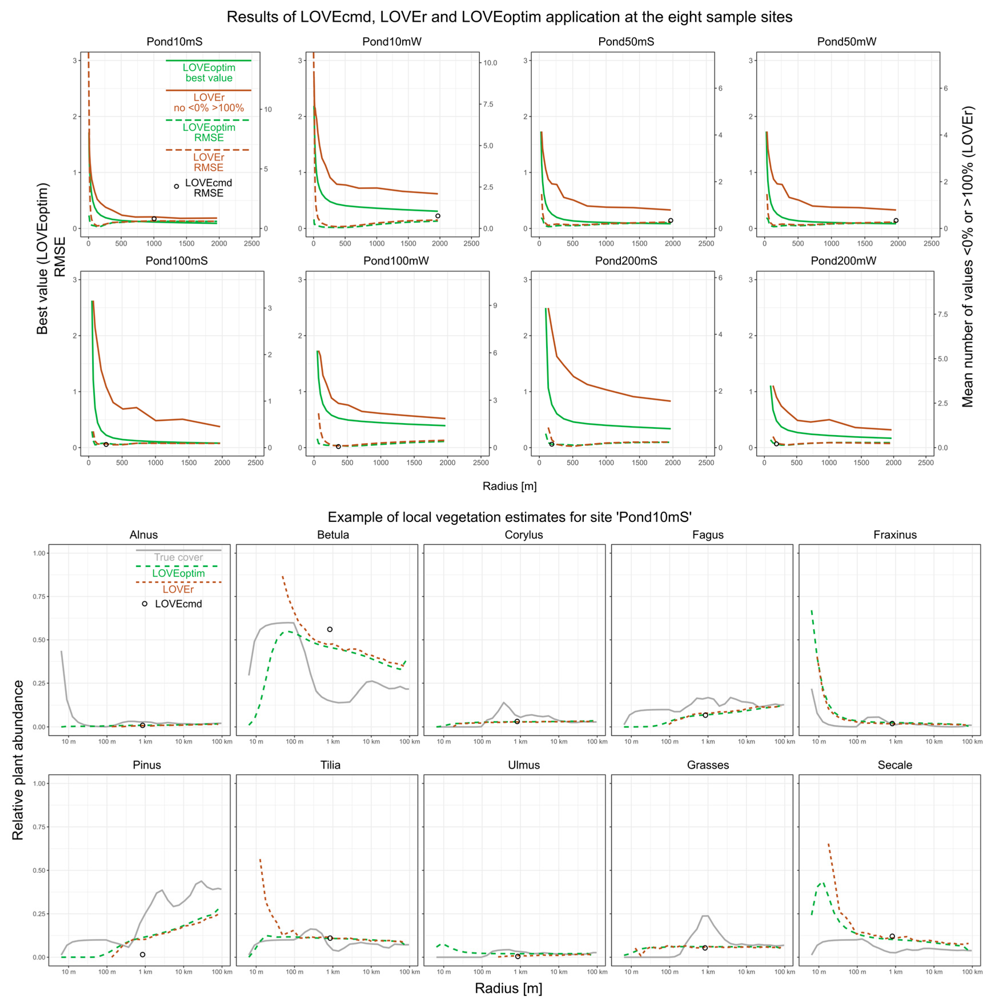
• The three software tools LOVEcmd, LOVEr and LOVEoptim produce roughly similar estimates of the local vegetation composition for our eight test sites (Figure 2). Low RMSE values, i.e., a high goodness-of-fit between the true and the reconstructed cover estimates support that LOVEr is a suitable implementation of the original LOVE model in R and that LOVEoptim is a suitable alternative numerical approach. LOVEoptim produces slightly more accurate estimates than LOVEr, particularly for calculations with the innermost rings only. One likely reason is that particularly for small local areas, LOVEr produces many cover estimates smaller than 0% or greater than 100%, whereas LOVEoptim always produces estimates between 0 and 100%. For LOVEcmd, we only show cover estimates for the ‘necessary source area of pollen’ (NSAP), as given by the ‘LRA.LOVE.v6.2.4.exe’ software. Those results are less accurate than the LOVEr and LOVEoptim estimates, particularity for the smaller sites.
• LOVEr and LOVEoptim produce best results when the rings until about 100–500 m distance are included as local. We would expect that the distance with the best results increases with basin size, but there is only weak evidence for such a relationship in the present results.
• The presence of a distinct shore vegetation with abundant Alnus and Fraxinus has only minor disturbing effects. For ‘Pond50mS’ and ‘Pond100mS’, the models show slightly too high local vegetation proportions of Alnus and Fraxinus, apparently due to their high cover on the lakeshore. In other cases, such effects are not observed.
• Errors in the reconstructed cover are largest for those taxa that show the largest changes in abundance with distance from the sample site, for example, for Betula in ‘Pond10mS’.
• When all rings are included in the calculations, the results of LOVEr and LOVEoptim tend to reflect, with some deviation, regional vegetation composition.

4. Discussion

In our simulated landscape setting, both LOVEr and LOVEoptim have proven to be useful tools for local scale vegetation reconstruction with pollen records from small sample sites. The main practical advantage of both R tools is their easier application. R scripts allow for the easy calculation of series with, for example, different sets of pollen types or different parameter settings, which are useful to explore the robustness of the results. Also, the effects of variations in the production and the dispersal of pollen may be studied. Moreover, the additional manual application of REVEALS is not required anymore. The model output is readily available for data analysis and presentation, e.g., in R. Finally, as the present example shows, R is a suitable platform to create realistic landscape scenarios from digital maps for the extensive testing of LOVEr and LOVEoptim. Such tests may involve landscapes with different vegetation patterns and different vegetation compositions.

LOVEoptim relies on fewer mathematical assumptions, and is, therefore, more widely applicable than the original LOVE model and LOVEr. Our implementation of LOVEoptim also provides greater flexibility in the calculations. The option to provide the land cover classes present in each individual ring allows to account for the landscape pattern in the vicinity of small sites, for example the presence of lakes or wetlands. By excluding wetland areas and—if distinguishable—wetland pollen taxa, a reconstruction may solely focus on the terrestrial vegetation. In the future, the approach may be further developed in this direction to also reconstruct vegetation patterns at the local scale, similar to the existing forward-modeling approaches such as the Extended Downscaling Approach and the Multiple Scenario approach [14,15].

4.1. Spatial Aspects

A key question in the application of LOVE is: which area’s vegetation is reflected in the reconstruction? Two concepts have been proposed to determine that area—the ‘relevant source area of pollen’ (RSAP) and the ‘necessary source area of pollen’ (NSAP). We did not use the RSAP here, because it can only be estimated using modern day vegetation estimates and pollen data, it cannot be estimated in the past. Moreover, theoretical considerations and observations show that the RSAP is primarily a measure of vegetation patch size—the RSAP increases with the vegetation patch size in a landscape [16]. In the landscape of northern Germany, with very large landscape and vegetation patterns as a result of past glacial activity, the RSAP tends to be very large [17]. In actuality, the size of the area reflected in local-scale reconstructions is rather determined by the pollen dispersal pattern than by the vegetation patch size.

Following unpublished notes on the LRA.LOVE.v6.2.4 software, the NSAP is the smallest local area for which LOVE does not produce outliers (cover estimates smaller than 0% or larger than 100%). In our tests, LOVEcmd produces large NSAPs for the small sites and small NSAPs for the larger sites. This behavior is obviously not related to vegetation patterns, as small and large sites occur in the western and in the southern group of sites. We also inspected the number of outliers to evaluate the performance of LOVEr, but used the best values (=log-Euclidean distance between modeled and true pollen composition after optimization) as a potential metric to evaluate the performance of LOVEoptim. Both values decline with each ring that is added as local, until the largest ring. The RMSE of the true versus the reconstructed local vegetation composition instead indicates that those reconstructions are most accurate that only include the rings until to 100–500 m distance. This mismatch suggests that the number of outliers and the best values do not clearly indicate the spatial scale of the reconstruction. However, the best values, and less clearly, the number of outliers, decline rapidly until about the distance of the best matching reconstruction, i.e., 100–500 m, and then decline much slower beyond that distance. We cannot evaluate whether this flattening of the curve is indeed indicative or just random. To prove such a relationship, further tests in different landscapes and with different vegetation types are needed.

Theory predicts that the area best represented in the pollen rain of a sample site increases with the diameter of the lake or peatland sampled [7]. Our results do not clearly show such a relationship, which may have several reasons. The influence of basin size may indeed be weak for the size class of the sites used in our tests, i.e., 10 to 200 m in diameter. A high contribution of (extra) local pollen in lakes with a diameter of about 50–200 m, probably originating from within ~300 m distance from the lakes, has been observed for example by [18]. On the other hand, pollen records from forest hollows with less than 10 m in diameter tend to mainly reflect vegetation composition within only about 10–50 m distance [2,4,19]. The local component of pollen deposition appears to be more important in such forest hollows than in our similarly small simulated sites. One reason for this may be that the dispersal model chosen in our test does not fully adequately depict deposition under closed canopies as it does not consider, for example, pollen washed into small basins by rainwater from the plants themselves or from the shore. Also, trees growing in half-open conditions at lake shores likely produce more pollen than trees growing in a dense stand [20]. This effect has a greater impact in very small sites than in larger ones. Future experiments should try to include such variations in pollen production and additional modes of pollen dispersal to study the effects.

4.2. Vegetation Patchiness

Theory predicts and previous tests have shown that LOVE performs best in landscapes with uniform vegetation composition and a fine-grained vegetation pattern [3]. The present tests use a landscape from northern Germany that is instead characterized by coarse vegetation patterns and inhomogeneous vegetation composition. For example, at the site ‘Pond10mS’, the vegetation composition at the edge of the basin (with much Alnus) is very different from the vegetation composition 100 m away (with much Betula) and 1000 m away (with more Pinus and grasses) (Figure 1 and Figure 2). In such situations, there is obviously no true reconstruction because the vegetation at all these distances influences the total pollen deposition. Simulations such as those presented here can help to understand how local scale reconstructions work in such landscapes and whether their application is useful at all. In the above example, the reconstruction appears to predominately reflect the Betula-rich vegetation within ~100 m distance. Whether this result is realistic needs further evaluation because, as mentioned above, our pollen dispersal simulations may underestimate the pollen deposition of nearby vegetation.

4.3. Error Estimates

For LOVEr and LOVEoptim, we have chosen to determine error estimates via repeated calculations with noise added in the pollen counts and pollen productivity estimates. We are aware that the resulting error margins are incomplete and do not fully reflect the magnitude of errors that may be present in local vegetation estimates. Our approach likely well reflects the errors related to the actual counts of a pollen sample with a given pollen sum, but additional errors in pollen data may be present due to the sample selection, preparation and so on. Also, errors in pollen productivity estimates obviously underestimate true uncertainty, as the standard errors given are usually much smaller than variations between pollen productivity studies. Moreover, on the local scale, variations in pollen productivity among individual plants, due to, for example, differences in age, genetics and site conditions, are much more relevant than on the regional scale. Finally, as mentioned above, the LOVE model is based on the assumption of homogeneous vegetation composition. Tests like those presented here may help to estimate the errors resulting from violations of that assumption.

5. Conclusions

The presented R-implementation of the LOVE model, LOVEr, and the adapted numerical approach, LOVEoptim, both allow for more user-friendly and faster local-scale vegetation reconstructions with pollen data from small sites. Due to its fewer mathematical assumptions, LOVEoptim is more widely applicable and offers greater flexibility in calculations than the original LOVE model.

R is a suitable platform for setting up realistic landscape scenarios to test the application of LOVEr and LOVEoptim. Such scenarios are firstly useful to explore whether a given study setting is indeed suitable for LOVE/LOVEoptim reconstructions. They also help to explore, for example, the impact of uncertainty in pollen productivity estimates. In our simulations, the ‘necessary source area of pollen’ (NSAP) does not reflect the spatial scale of the reconstructed vegetation. Further testing and a better understanding of pollen dispersal patterns are needed to improve our understanding of the spatial scale of vegetation reconstructed using the LOVE/LOVEoptim approach.

References

- Janssen, C.R. Recent Pollen Spectra from the Deciduous and Coniferous-Deciduous Forests of Northeastern Minnesota: A Study in Pollen Dispersal. Ecology 1966, 47, 804–825. [Google Scholar] [CrossRef]
- Andersen, S.T. Tree-Pollen Rain in a Mixed Deciduous Forest in South Jutland (Denmark). Rev. Palaeobot. Palynol. 1967, 3, 267–275. [Google Scholar] [CrossRef]
- Sugita, S. Theory of Quantitative Reconstruction of Vegetation II: All You Need Is LOVE. Holocene 2007, 17, 243–257. [Google Scholar] [CrossRef]
- Mrotzek, A.; Couwenberg, J.; Theuerkauf, M.; Joosten, H. MARCO POLO—A New and Simple Tool for Pollen-Based Stand-Scale Vegetation Reconstruction. Holocene 2017, 27, 321–330. [Google Scholar] [CrossRef]
- R Core Team. R: A Language and Environment for Statistical Computing; R Foundation for Statistical Computing: Vienna, Austria, 2023. [Google Scholar]
- Oelbüttel, M.; Filipović, D.; Kneisel, J.; Kirleis, W. Inside or Outside the House? On the Spatial Organisation of Plant-Related Activities at the Late Bronze Age Settlement of Dobbin 27, Northern Germany. Prähistorische Z. 2024; in press. [Google Scholar] [CrossRef]
- Prentice, I.C. Pollen Representation, Source Area, and Basin Size: Toward a Unified Theory of Pollen Analysis. Quat. Res. 1985, 23, 76–86. [Google Scholar] [CrossRef]
- Sugita, S. Pollen Representation of Vegetation in Quaternary Sediments: Theory and Method in Patchy Vegetation. J. Ecol. 1994, 82, 881–897. [Google Scholar] [CrossRef]
- Sugita, S. Theory of Quantitative Reconstruction of Vegetation I: Pollen from Large Sites REVEALS Regional Vegetation Composition. Holocene 2007, 17, 229–241. [Google Scholar] [CrossRef]
- Eddelbuettel, D. RcppDE: Global Optimization by Differential Evolution in C++; 2022. Available online: https://cran.r-project.org/web/packages/RcppDE/ (accessed on 23 February 2024).
- Feeser, I.; Dörfler, W.; Czymzik, M.; Dreibrodt, S. A Mid-Holocene Annually Laminated Sediment Sequence from Lake Woserin: The Role of Climate and Environmental Change for Cultural Development during the Neolithic in Northern Germany. Holocene 2016, 26, 947–963. [Google Scholar] [CrossRef]
- Czymzik, M.; Dreibrodt, S.; Feeser, I.; Adolphi, F.; Brauer, A. Mid-Holocene Humid Periods Reconstructed from Calcite Varves of the Lake Woserin Sediment Record (North-Eastern Germany). Holocene 2016, 26, 935–946. [Google Scholar] [CrossRef]
- Kuparinen, A.; Markkanen, T.; Riikonen, H.; Vesala, T. Modeling Air-Mediated Dispersal of Spores, Pollen and Seeds in Forested Areas. Ecol. Model. 2007, 208, 177–188. [Google Scholar] [CrossRef]
- Theuerkauf, M.; Couwenberg, J. The extended downscaling approach: A new R-tool for pollen-based reconstruction of vegetation patterns. Holocene 2017, 27, 1252–1258. [Google Scholar] [CrossRef]
- Bunting, M.J.; Farrell, M.; Bayliss, A.; Marshall, P.; Whittle, A. Maps from Mud—Using the Multiple Scenario Approach to Reconstruct Land Cover Dynamics from Pollen Records: A Case Study of Two Neolithic Landscapes. Front. Ecol. Evol. 2018, 6, 36. [Google Scholar] [CrossRef]
- Bunting, M.J.; Gaillard, M.-J.; Sugita, S.; Middleton, R.; Broström, A. Vegetation Structure and Pollen Source Area. Holocene 2004, 14, 651–660. [Google Scholar] [CrossRef]
- Theuerkauf, M. Fine Scaled Vegetation Patterns in the Lateglacial and Early Holocene of NE Germany—Novel GIS Based Approaches. Ph.D. Dissertation, University of Greifswald, Greifswald, 2013. [Google Scholar]
- Matthias, I.; Giesecke, T. Insights into Pollen Source Area, Transport and Deposition from Modern Pollen Accumulation Rates in Lake Sediments. Quat. Sci. Rev. 2014, 87, 12–23. [Google Scholar] [CrossRef]
- Andersen, S.T. The Relative Pollen Productivity and Pollen Representativity of North European Trees and Correction Factors for Tree Pollen Spectra. Dan. Geol. Undersøgelser Ser. II 1970, 96, 1–99. [Google Scholar]
- Feeser, I.; Dörfler, W. The Glade Effect: Vegetation Openness and Structure and Their Influences on Arboreal Pollen Production and the Reconstruction of Anthropogenic Forest Opening. Anthropocene 2014, 8, 92–100. [Google Scholar] [CrossRef]