
Fluvial Response to Environmental Change in Sub-Tropical Australia over the Past 220 Ka

Abstract
:1. Introduction
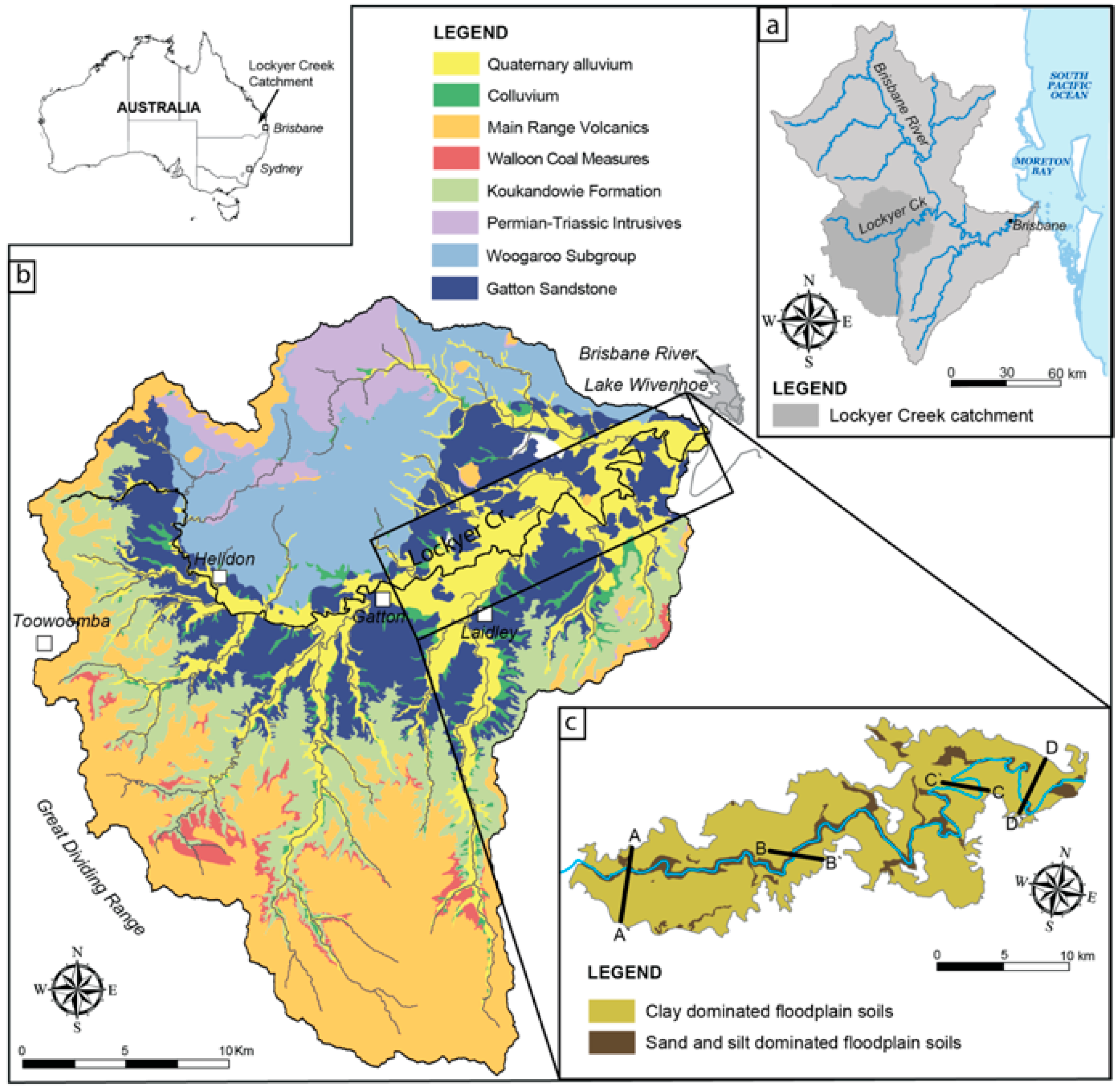
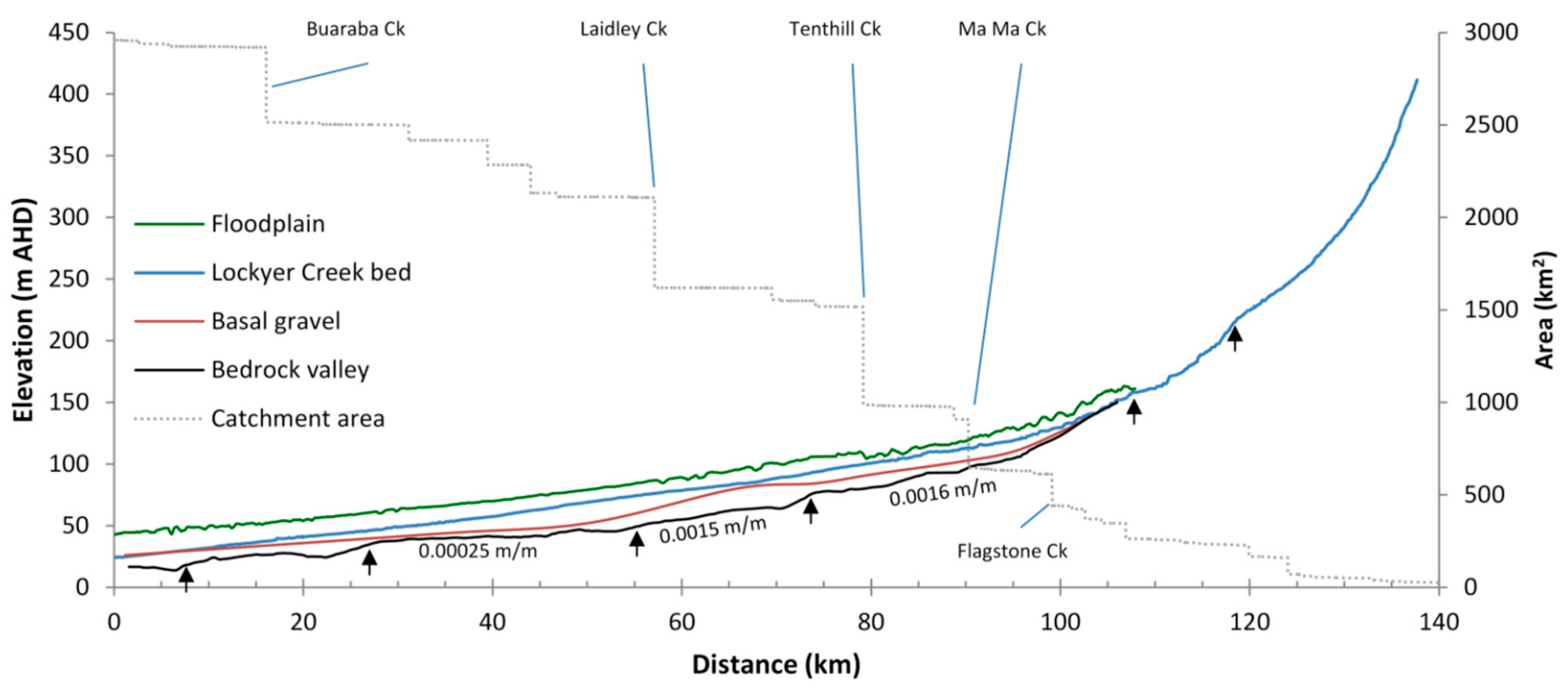
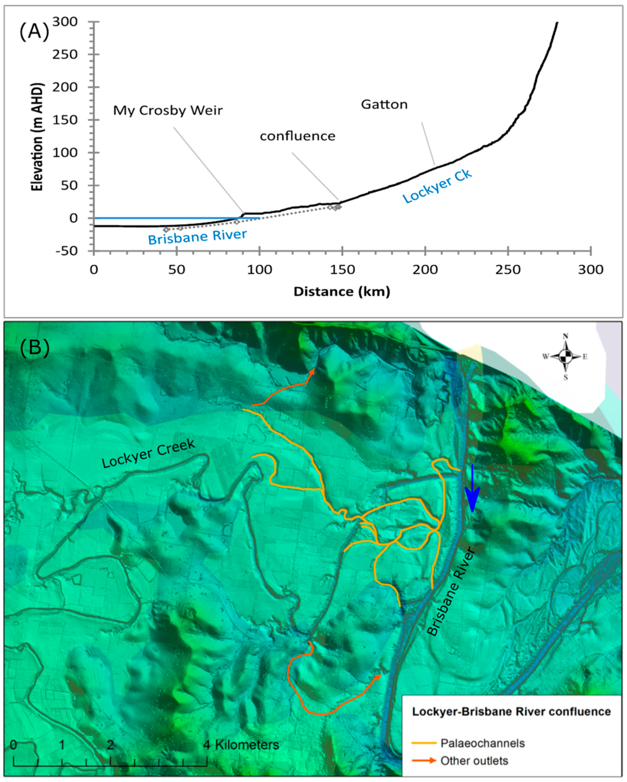
Regional Setting
2. Materials and Methods
2.1. OSL Dating
Visualisation of OSL Ages
2.2. Radiocarbon Dating
2.3. Aggradation Rates
3. Results
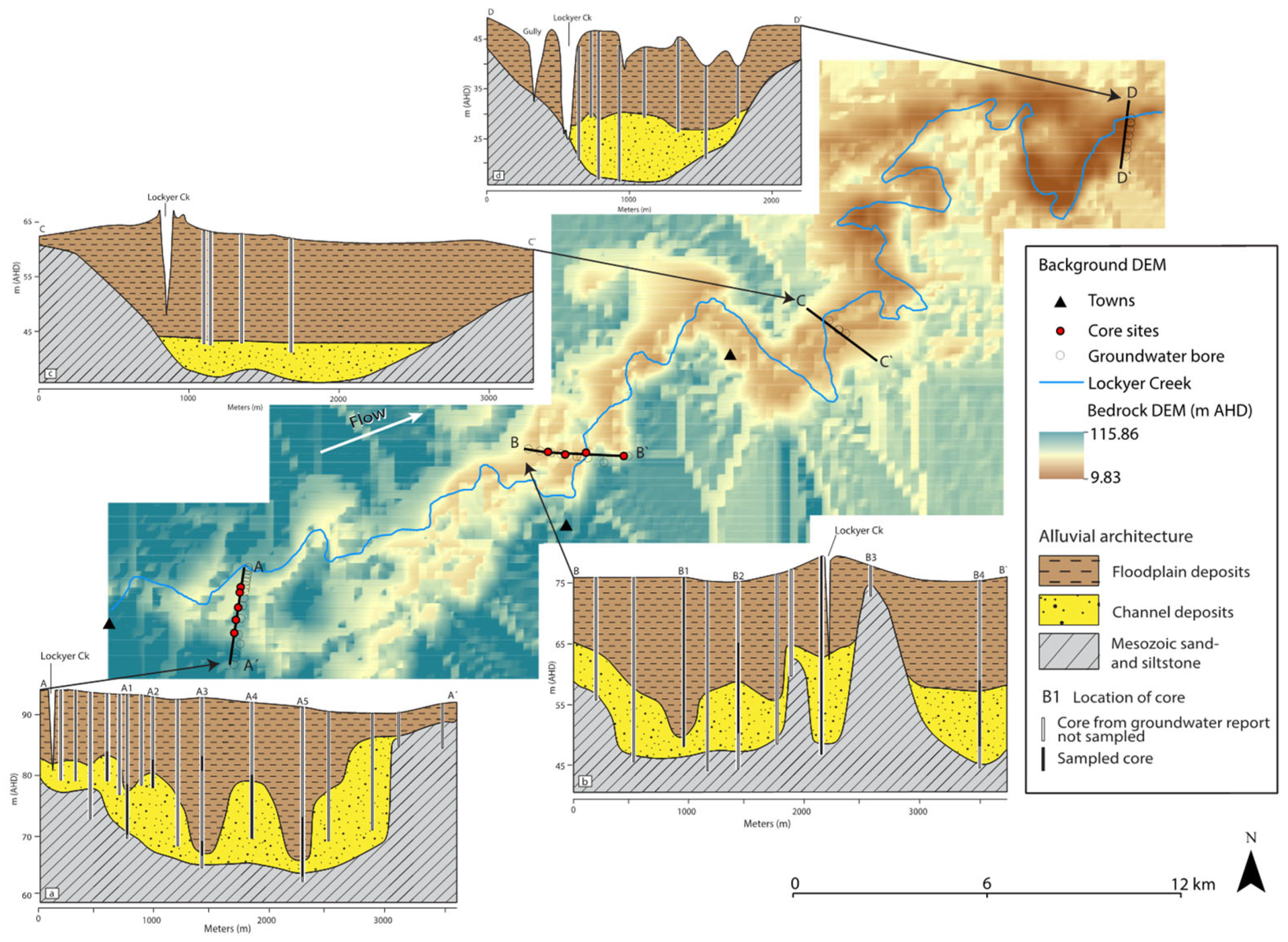
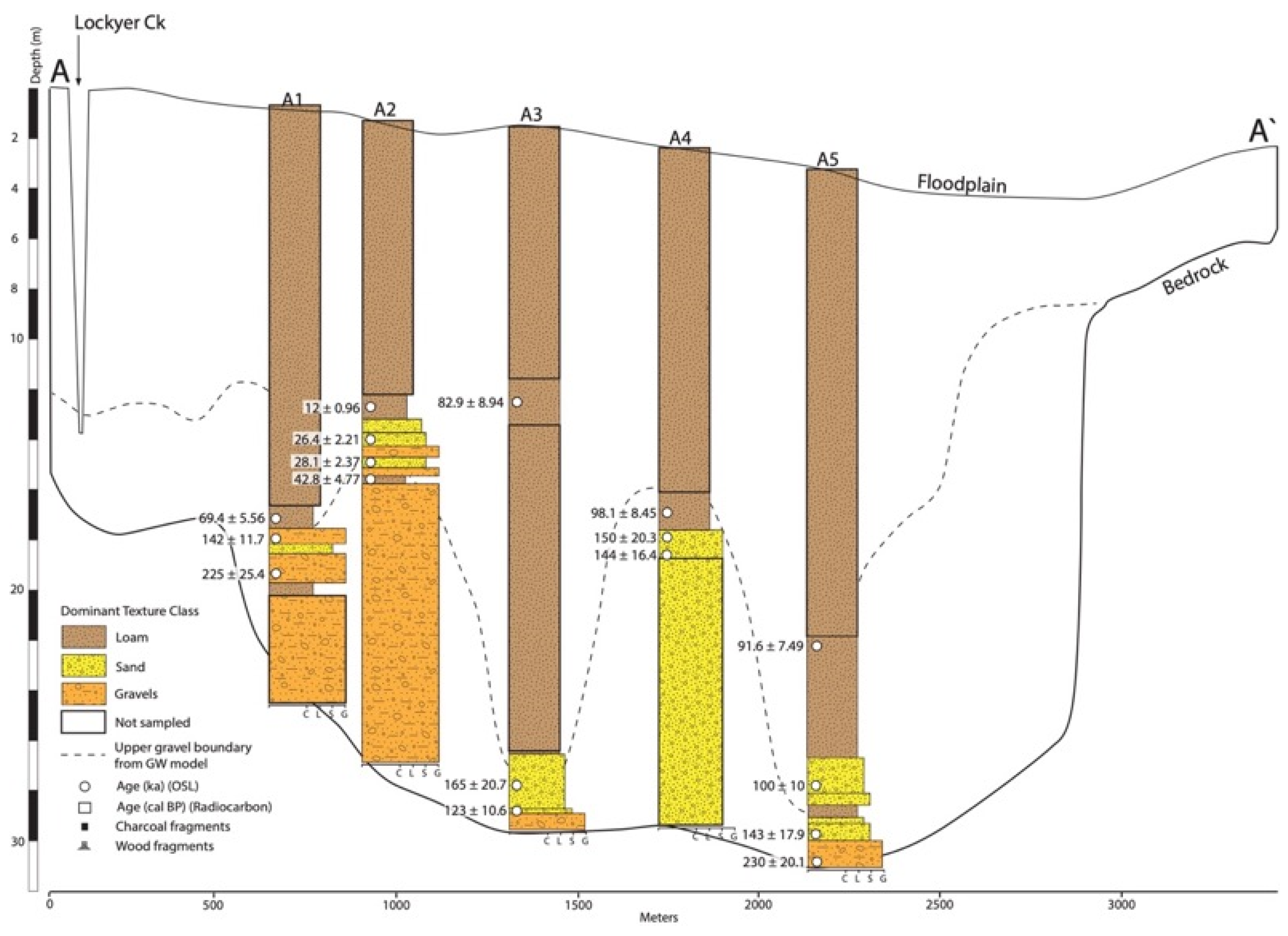
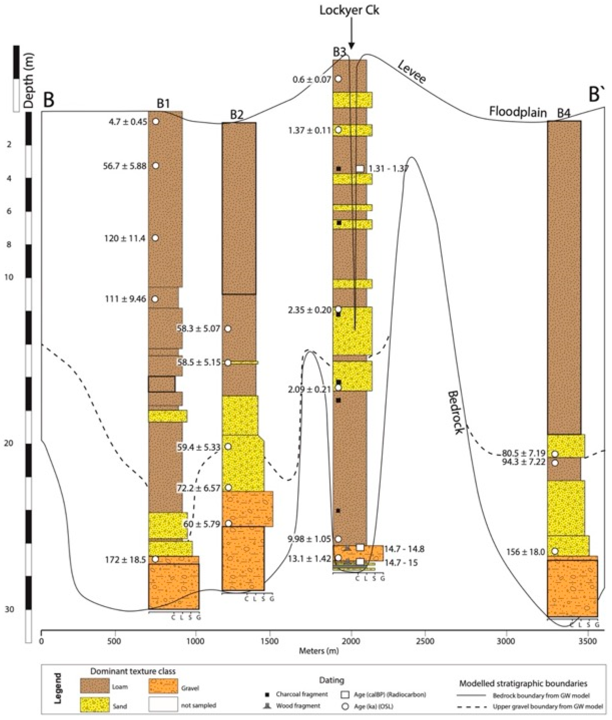
3.1. Valley Fill Chronostratigraphy
3.1.1. Coarse Channel Deposits
3.1.2. Fine-Grained Units
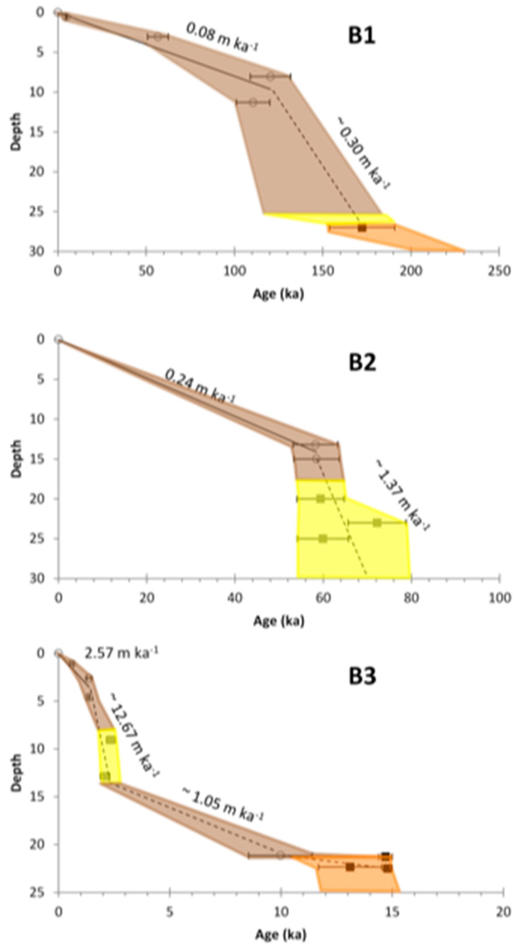
3.1.3. Aggradation Rates
4. Discussion
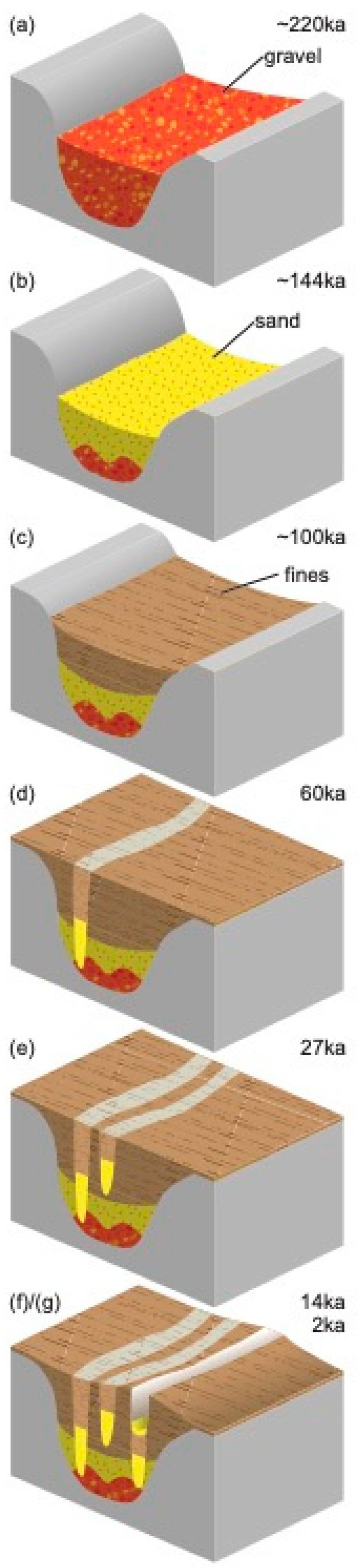
4.1. Phases of Incision and Aggradation
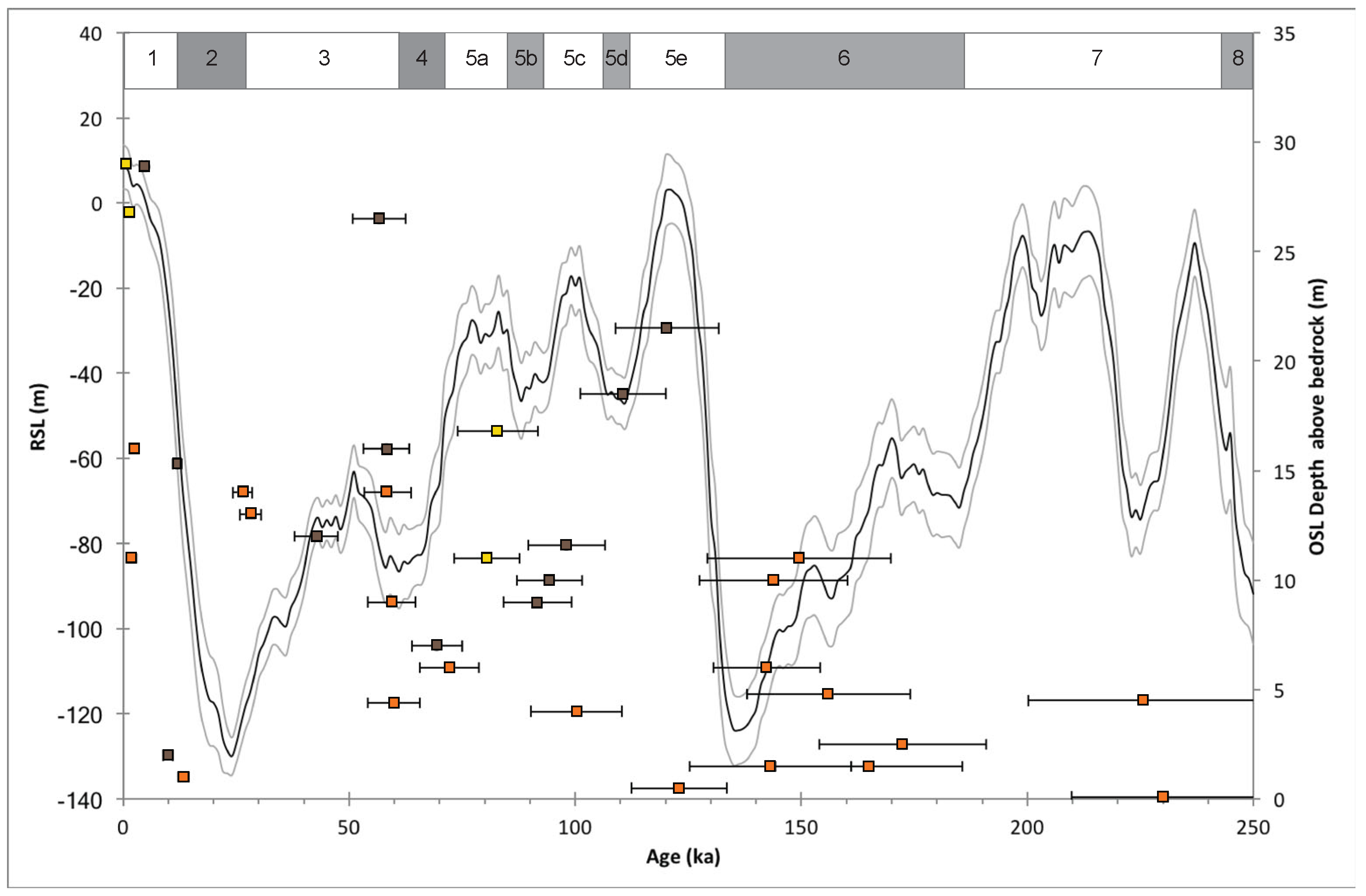
4.2. Base-Level Adjustments
5. Conclusions
Supplementary Materials
Author Contributions
Funding
Data Availability Statement
Acknowledgments
Conflicts of Interest
References
- Westaway, R.; Bridgland, D.R.; Sinha, R.; Demir, T. Fluvial sequences as evidence for landscape and climatic evolution in the Late Cenozoic: A synthesis of data from IGCP 518. Glob. Planet. Chang. 2009, 68, 237–253. [Google Scholar] [CrossRef]
- Bridgland, D.R.; Keen, D.H.; Westaway, R. Global correlation of late Cenozoic fluvial deposits: A synthesis of data from IGCP 449. Quat. Sci. Rev. 2007, 26, 2694–2700. [Google Scholar] [CrossRef]
- Macklin, M.G.; Lewin, J.; Woodward, J.C. The fluvial record of climate change. Philos. Trans. R. Soc. Lond. A 2012, 370, 2143–2172. [Google Scholar] [CrossRef] [PubMed]
- Nanson, G.; Cohen, T.J.; Doyle, C.J.; Price, D.M. Alluvial evidence of major late Quaternary climate and flow regime changes on the coastal rivers of New South Wales, Australia. In Palaeohydrology: Understanding Global Change; Gregory, K.J., Benito, G., Eds.; Wiley & Sons: Hoboken, NJ, USA, 2003; pp. 233–258. [Google Scholar]
- Nanson, G.C.; Price, D.M.; Short, S.A. Wetting and drying of Australia over the past 300 ka. Geology 1992, 20, 791–794. [Google Scholar] [CrossRef]
- Petherick, L.; Bostock, H.; Cohen, T.J.; Fitzsimmons, K.; Tibby, J.; Fletcher, M.S.; Moss, P.; Reeves, J.; Mooney, S.; Barrows, T.; et al. Climatic records over the past 30 ka from temperate Australia—A synthesis from the Oz-INTIMATE workgroup. Quat. Sci. Rev. 2013, 74, 58–77. [Google Scholar] [CrossRef]
- Kemp, J.; Rhodes, E.J. Episodic fluvial activity of inland rivers in southeastern Australia: Palaeochannel systems and terraces of the Lachlan River. Quat. Sci. Rev. 2010, 29, 732–752. [Google Scholar] [CrossRef]
- Kemp, J.; Spooner, N.A. Evidence for regionally wet conditions before the LGM in southeast Australia: OSL ages from a large palaeochannel in the Lachlan Valley. J. Quat. Sci. 2007, 22, 423–427. [Google Scholar] [CrossRef]
- Page, K.; Nanson, G.; Price, D. Chronology of Murrumbidgee River palaeochannels on the Riverine Plain, southeastern Australia. J. Quat. Sci. 1996, 11, 311–326. [Google Scholar] [CrossRef]
- Page, K.J.; Nanson, G.C.; Price, D.M. Thermoluminescence chronology of late quaternary deposition on the riverine plain of South-Eastern Australia. Aust. Geogr. 1991, 22, 14–23. [Google Scholar] [CrossRef]
- Hughes, K.; Croke, J. How did rivers in the wet tropics (NE Queensland, Australia) respond to climate changes over the past 30,000 years? J. Quat. Sci. 2017, 32, 744–759. [Google Scholar] [CrossRef]
- Cheetham, M.D.; Bush, R.T.; Keene, A.F.; Erskine, W.D. Nonsynchronous, episodic incision: Evidence of threshold exceedance and complex response as controls of terrace formation. Geomorphology 2010, 123, 320–329. [Google Scholar] [CrossRef]
- Cohen, T.J.; Nanson, G.C. Mind the gap: An absence of valley-fill deposits identifying the Holocene hypsithermal period of enhanced flow regime in southeastern Australia. Holocene 2007, 17, 411–418. [Google Scholar] [CrossRef]
- Powell, B. Nature, Distribution and Origin of Soils on an Alluvial Landscape in the Lockyer Valley, South-East Queensland; University of New England: Portland, OR, USA, 1987. [Google Scholar]
- Croke, J.; Todd, P.; Thompson, C.; Watson, F.; Denham, R.; Khanal, G. The use of multi temporal LiDAR to assess basin-scale erosion and deposition following the catastrophic January 2011 Lockyer flood, SE Queensland, Australia. Geomorphology 2013, 184, 111–126. [Google Scholar] [CrossRef]
- Kiem, A.S.; Franks, S.W.; Kuczera, G. Multi-decadal variability of flood risk. Geophys. Res. Lett. 2003, 30, 36-1–36-4. [Google Scholar] [CrossRef]
- Thompson, C.; Croke, J. The geomorphic effects, flood power and channel competence of a catastrophic flood in confined and unconfined reaches of the upper Lockyer valley, south east Queensland, Australia. Geomorphology 2013, 197, 156–169. [Google Scholar] [CrossRef]
- Thompson, C.; Croke, J.; Dent, C. Potential Impacts of levee in construction in the Lockyer Valley. In Proceedings of the 7th Australian Stream Management Conference, Townsville, QLD, Australia, 27–30 July 2014; p. 7. [Google Scholar]
- Apan, A.A.; Raine, S.R.; Paterson, M.S. Mapping and analysis of changes in the riparian landscape structure of the Lockyer Valley catchment, Queensland, Australia. Landsc. Urban Plan. 2002, 59, 43–57. [Google Scholar] [CrossRef]
- Raiber, M.; Lewis, S.; Cendon, D.; Cui, T.; Cox, M.; Gilfedder, M.; Rassam, D. Significance of the connection between bedrock, alluvium and streams: A spatial and temporal hydrogeological and hydrogeochemical assessment from Queensland, Australia. J. Hydrol. 2019, 569, 666–684. [Google Scholar] [CrossRef]
- Folk, R.L. The Distinction between Grain Size and Mineral Composition in Sedimentary-Rock Nomenclature. J. Geol. 1954, 62, 344–359. [Google Scholar] [CrossRef]
- Olley, J.M.; Pietsch, T.; Roberts, R.G. Optical dating of Holocene sediments from a variety of geomorphic settings using single grains of quartz. Geomorphology 2004, 60, 337–358. [Google Scholar] [CrossRef]
- Pietsch, T.J. Optically stimulated luminescence dating of young (<500 years old) sediments: Testing estimates of burial dose. Quat. Geochronol. 2009, 4, 406–422. [Google Scholar] [CrossRef]
- Galbraith, R.F.; Laslett, G.M. Statistical models for mixed fission track ages. Nucl. Tracks Radiat. Meas. 1993, 21, 459–470. [Google Scholar] [CrossRef]
- Galbraith, R.F.; Roberts, R.G.; Laslett, G.M.; Yoshida, H.; Olley, J.M. Optical Dating Of Single And Multiple Grains Of Quartz From Jinmium Rock Shelter, Northern Australia: Part I, Experimental Design And Statistical Models. Archaeometry 1999, 41, 339–364. [Google Scholar] [CrossRef]
- Roberts, H.M.; Wintle, A.G. Equivalent dose determinations for polymineralic fine-grains using the SAR protocol: Application to a Holocene sequence of the Chinese Loess Plateau. Quat. Sci. Rev. 2001, 20, 859–863. [Google Scholar] [CrossRef]
- Arnold, L.J.; Roberts, R.G.; Galbraith, R.F.; DeLong, S.B. A revised burial dose estimation procedure for optical dating of young and modern-age sediments. Quat. Geochronol. 2009, 4, 306–325. [Google Scholar] [CrossRef]
- Murray, A.S.; Marten, R.; Johnston, A.; Martin, P. Analysis for naturally occuring radionuclides at environmental concentrations by gamma spectrometry. J. Radioanal. Nucl. Chem. 1987, 115, 263. [Google Scholar] [CrossRef]
- Stokes, S.; Hetzel, R.; Bailey, R.M.; Mingxin, T. Combined IRSL-OSL single aliquot regeneration (SAR) equivalent dose (De) estimates from source proximal Chinese loess. Quat. Sci. Rev. 2003, 22, 975–983. [Google Scholar] [CrossRef]
- Guérin, G.; Mercier, N.; Nathan, R.; Adamiec, G.; Lefrais, Y. On the use of the infinite matrix assumption and associated concepts: A critical review. Radiat. Meas. 2012, 47, 778–785. [Google Scholar] [CrossRef]
- Prescott, J.R.; Hutton, J.T. 1994Cosmic ray contributions to dose rates for luminescence and ESR dating: Large depths and long-term time variations. Radiat. Meas. 1994, 23, 497–500. [Google Scholar] [CrossRef]
- Bowler, J.M.; Johnston, H.; Olley, J.M.; Prescott, J.R.; Roberts, R.G.; Shawcross, W.; Spooner, N.A. New ages for human occupation and climatic change at Lake Mungo, Australia. Nature 2003, 421, 837–840. [Google Scholar] [CrossRef]
- Vermeesch, P. On the visualisation of detrital age distributions. Chem. Geol. 2012, 312–313, 190–194. [Google Scholar] [CrossRef]
- Abramson, I.S. On Bandwidth Variation in Kernel Estimates-A Square Root Law. Ann. Stat. 1982, 10, 1217–1223. [Google Scholar] [CrossRef]
- Jann, B. Univariate Kernel Density Estimation; Statistical Software Component S456410; College Department of Economics: Chestnut Hill, MA, USA, 2007; Available online: http://fmwww.bc.edu/RePEc/bocode/k/kdens.pdf (accessed on 2 January 2024).
- Hall, P. Large Sample Optimality of Least Squares Cross-Validation in Density Estimation. Ann. Stat. 1983, 11, 1156–1174. [Google Scholar] [CrossRef]
- Sheather, S.J. Density Estimation. Stat. Sci. 2004, 19, 588–597. [Google Scholar] [CrossRef]
- Beta Analytic Inc. Introduction to Radiocarbon Determination by the Accelerator Mass Spectrometry Method; Beta Analytic Inc.: Miami, FL, USA, 2015. [Google Scholar]
- Talma, A.S.; Vogel, J.C. A simplified approach to calibrating 14C dates. Radiocarbon 1993, 35, 317–322. [Google Scholar] [CrossRef]
- Hogg, A.G.; Hua, Q.; Blackwell, P.G.; Niu, M.; Buck, C.E.; Guilderson, T.P.; Heaton, T.J.; Palmer, J.G.; Reimer, P.J.; Reimer, R.W.; et al. SHCal13 Southern Hemisphere Calibration, 0–50,000 Years cal BP. Radiocarbon 2013, 55, 1889–1903. [Google Scholar] [CrossRef]
- Cohen, T.J.; Nanson, G.C. Topographically associated but chronologically disjunct late Quaternary floodplains and terraces in a partly confined valley, south-eastern Australia. Earth Surf. Process. Landf. 2008, 33, 424–443. [Google Scholar] [CrossRef]
- Croke, J.; Jansen, J.D.; Amos, K.; Pietsch, T.J. A 100 ka record of fluvial activity in the Fitzroy River Basin, tropical northeastern Australia. Quat. Sci. Rev. 2011, 30, 1681–1695. [Google Scholar] [CrossRef]
- Pietsch, T.J.; Nanson, G.C.; Olley, J.M. Late Quaternary changes in flow-regime on the Gwydir distributive fluvial system, southeastern Australia. Quat. Sci. Rev. 2013, 69, 168–180. [Google Scholar] [CrossRef]
- Thomsen, K.J.; Murray, A.S.; Buylaert, J.P.; Jain, M.; Hansen, J.H.; Aubry, T. Testing single-grain quartz OSL methods using sediment samples with independent age control from the Bordes-Fitte rockshelter (Roches d’Abilly site, Central France). Quat. Geochronol. 2016, 31, 77–96. [Google Scholar] [CrossRef]
- Nanson, G.C.; Price, D.M.; Jones, B.G.; Maroulis, J.C.; Coleman, M.; Bowman, H.; Cohen, T.J.; Pietsch, T.J.; Larsen, J.R. Alluvial evidence for major climate and flow regime changes during the middle and late Quaternary in eastern central Australia. Geomorphology 2008, 101, 109–129. [Google Scholar] [CrossRef]
- Daley, J.; Croke, J.; Thompson, C.; Cohen, T.; Macklin, M.; Sharma, A. Late Quaternary channel and floodplain formation in a partly confined subtropical river, eastern Australia. J. Quat. Sci. 2017, 32, 729–743. [Google Scholar] [CrossRef]
- Cohen, T.J.; Nanson, G.C.; Jansen, J.D.; Jones, B.G.; Jacobs, Z.; Treble, P.; Price, D.M.; May, J.-H.; Smith, A.M.; Ayliffe, L.K.; et al. Continental aridification and the vanishing of Australia’s megalakes. Geology 2011, 39, 167–170. [Google Scholar] [CrossRef]
- McGowan, H.A.; Petherick, L.M.; Kamber, B.S. Aeolian sedimentation and climate variability during the late Quaternary in southeast Queensland, Australia. Palaeogeogr. Palaeoclimatol. Palaeoecol. 2008, 265, 171–181. [Google Scholar] [CrossRef]
- Moss, P.T.; Tibby, J.; Petherick, L.; McGowan, H.; Barr, C. Late Quaternary vegetation history of North Stradbroke Island, Queensland, eastern Australia. Quat. Sci. Rev. 2013, 74, 257–272. [Google Scholar] [CrossRef]
- Petherick, L.M.; Moss, P.T.; McGowan, H.A. An extended Last Glacial Maximum in subtropical Australia. Quat. Int. 2016, 432, 1–12. [Google Scholar] [CrossRef]
- Reeves, J.M.; Barrows, T.T.; Cohen, T.J.; Kiem, A.S.; Bostock, H.C.; Fitzsimmons, K.E.; Jansen, J.D.; Kemp, J.; Krause, C.; Petherick, L.; et al. Climate variability over the last 35,000 years recorded in marine and terrestrial archives in the Australian region: An OZ-INTIMATE compilation. Quat. Sci. Rev. 2013, 74, 21–34. [Google Scholar] [CrossRef]
- Petherick, L.M.; McGowan, H.A.; Moss, P.T.; Kamber, B.S. Late Quaternary aridity and dust transport pathways in eastern Australia. Quat. Australas. 2008, 25, 2–11. [Google Scholar]
- Donders, T.H.; Wagner, F.; Visscher, H. Late Pleistocene and Holocene subtropical vegetation dynamics recorded in perched lake deposits on Fraser Island, Queensland, Australia. Palaeogeogr. Palaeoclimatol. Palaeoecol. 2006, 241, 417–439. [Google Scholar] [CrossRef]
- McGowan, H.; Marx, S.; Moss, P.; Hammond, A. Evidence of ENSO mega-drought triggered collapse of prehistory Aboriginal society in northwest Australia. Geophys. Res. Lett. 2012, 39, L22702. [Google Scholar] [CrossRef]
- Shulmeister, J.; Lees, B.G. Pollen evidence from tropical Australia for the onset of an ENSO-dominated climate at c. 4000 BP. Holocene 1995, 5, 10–18. [Google Scholar] [CrossRef]
- Spratt, R.M.; Lisiecki, L.E. A Late Pleistocene sea level stack. Clim. Past 2016, 12, 1079–1092. [Google Scholar] [CrossRef]
- Woolfe, K.L.; Larcombe, P.; Naish, T.; Purdon, R.G. Lowstand rivers need not incise the shelf: An example from the Great Barrier Reef, Australia, with implications for sequence stratigraphic models. Geology 1998, 26, 75–78. [Google Scholar] [CrossRef]
- Lewis, S.E.; Sloss, C.R.; Murray-Wallace, C.V.; Woodroffe, C.D.; Smithers, S.G. Post-glacial sea-level changes around the Australian margin: A review. Quat. Sci. Rev. 2013, 74, 115–138. [Google Scholar] [CrossRef]
- Daley, J.; Cohen, T. Climatically controlled river terraces in eastern Australia. Quaternary 2018, 1, 23. [Google Scholar] [CrossRef]
- Croke, J.; Fryirs, K.; Thompson, C. Channel–floodplain connectivity during an extreme flood event: Implications for sediment erosion, deposition, and delivery. Earth Surf. Process. Landf. 2013, 38, 1444–1456. [Google Scholar] [CrossRef]
- Croke, J.; Thompson, C.; Denham, R.; Haines, H.; Sharma, A.; Pietsch, T. Reconstructing a millennial-scale record of flooding in a single valley setting: The 2011 flood-affected Lockyer Valley, south east Queensland Australia. J. Quat. Sci. 2016, 31, 936–952. [Google Scholar] [CrossRef]


| Core | Lab ID | Field ID | 238U (Bq/Kg) | 226Ra (Bq/Kg) | 210Pb (Bq/Kg) | 228Ra (Bq/Kg) | 228Th (Bq/Kg) | 40K (Bq/Kg) | Dose Rate Total (Gy/Ka) | Estimated Dose (Gy) | Age (Ka) | † Age Model |
|---|---|---|---|---|---|---|---|---|---|---|---|---|
| A1 | 15-0210-054 | L6-1-110 | 21 ± 6 | 18 ± 2 | 15 ± 5 | 27 ± 3 | 26 ± 2 | 286 ± 20 | 1.62 ± 0.13 | 112 ± 2.09 | 69.35 ± 5.56 | a |
| 15-0210-055 | L6-2-150 | 10 ± 4 | 7 ± 1 | 9 ± 3 | 12 ± 1 | 13 ± 1 | 110 ± 10 | 0.83 ± 0.07 | 118 ± 2.44 | 142.39 ± 11.74 | a | |
| 15-0210-057 | L6-3-290 | 14 ± 5 | 14 ± 2 | 15 ± 4 | 16 ± 2 | 18 ± 2 | 132 ± 10 | 1.03 ± 0.09 | 231.4 ± 17.4 | 225.6 ± 25.4 | a | |
| A2 | 15-0210-059 | L8-1-110 | 8 ± 8 | 14 ± 2 | 5 ± 7 | 15 ± 3 | 21 ± 2 | 362 ± 26 | 1.73 ± 0.13 | 20.8 ± 0.64 | 12.01 ± 0.96 | a |
| 15-0210-060 | L8-2-150 | 11 ± 5 | 11 ± 2 | 8 ± 4 | 15 ± 3 | 14 ± 2 | 253 ± 18 | 1.39 ± 0.11 | 36.74 ± 1.25 | 26.40 ± 2.21 | a | |
| 15-0210-062 | L8-3-265 | 10 ± 3 | 8 ± 1 | 8 ± 3 | 10 ± 1 | 10 ± 1 | 203 ± 17 | 1.05 ± 0.08 | 29.62 ± 1.19 | 28.14 ± 2.37 | a | |
| 15-0210-066 | L8-4-450 | 18 ± 8 | 17 ± 3 | 13 ± 7 | 14 ± 3 | 19 ± 2 | 299 ± 25 | 1.45 ± 0.11 | 61.96 ± 4.92 | 42.80 ± 4.77 | a | |
| A3 | 15-0210-067 | L10-1-60 | 31 ± 10 | 19 ± 2 | 17 ± 7 | 28 ± 3 | 26 ± 2 | 351 ± 26 | 1.90 ± 0.15 | 157.3 ± 11.8 | 82.89 ± 8.94 | a |
| 15-0210-068 | L10-3-295 | 16 ± 9 | 11 ± 2 | 11 ± 9 | 16 ± 2 | 20 ± 2 | 299 ± 21 | 1.38 ± 0.10 | 227.4 ± 23 | 164.9 ± 20.68 | a | |
| 15-0210-069 | L10-5-470 | 12 ± 4 | 9 ± 1 | 9 ± 4 | 16 ± 2 | 17 ± 1 | 253 ± 21 | 1.20 ± 0.09 | 148 ± 6.53 | 122.99 ± 10.61 | a | |
| A4 | 15-0210-071 | L11-1-30 | 9 ± 8 | 11 ± 1 | 3 ± 9 | 26 ± 4 | 22 ± 2 | 279 ± 20 | 1.46 ± 0.11 | 143.3 ± 6.2 | 98.07 ± 8.45 | a |
| 15-0210-072 | L11-2-190 | 20 ± 8 | 11 ± 1 | 9 ± 6 | 19 ± 3 | 17 ± 1 | 295 ± 19 | 1.52 ± 0.11 | 227.2 ± 25.8 | 149.6 ± 20.3 | a | |
| 15-0210-073 | L11-2-230 | 6 ± 9 | 8 ± 2 | 9 ± 10 | 15 ± 3 | 18 ± 2 | 278 ± 23 | 1.42 ± 0.11 | 204.5 ± 17.2 | 143.90 ± 16.40 | a | |
| A5 | 15-0210-074 | L12-1-140 | 15 ± 5 | 15 ± 2 | 11 ± 4 | 15 ± 2 | 16 ± 1 | 254 ± 18 | 1.35 ± 0.10 | 124.0 ± 4.07 | 91.64 ± 7.49 | a |
| 15-0210-079 | L12-5-585 | 10 ± 7 | 10 ± 1 | 9 ± 7 | 15 ± 2 | 16 ± 1 | 279 ± 23 | 1.28 ± 0.09 | 128.8 ± 8.7 | 100.3 ± 10.0 | a | |
| 15-0210-080 | L12-6-770 | 6 ± 8 | 11 ± 2 | 12 ± 9 | 20 ± 3 | 21 ± 2 | 267 ± 21 | 1.21 ± 0.09 | 173 ± 17 | 143.11 ± 17.86 | a | |
| 15-0210-082 | L12-7-985 | 15 ± 6 | 10 ± 2 | 12 ± 6 | 15 ± 2 | 16 ± 1 | 260 ± 23 | 1.28 ± 0.10 | 294 ± 11.03 | 230.01 ± 20.13 | b | |
| B1 | 15-0210-001 | L1-1-56 | 21 ± 9 | 15 ± 2 | 10 ± 7 | 21 ± 4 | 20 ± 2 | 242 ± 18 | 1.36 ± 0.11 | 6.40 ± 0.35 | 4.700 ± 0.450 | b |
| 15-0210-004 | L1-6-805 | 17 ± 5 | 14 ± 2 | 12 ± 4 | 19 ± 2 | 20 ± 1 | 221 ± 19 | 1.26 ± 0.10 | 151.4 ± 7.4 | 120.35 ± 11.41 | a | |
| 15-0210-005 | L1-10-1293 | 21 ± 7 | 16 ± 2 | 16 ± 6 | 25 ± 5 | 27 ± 2 | 240 ± 16 | 1.38 ± 0.12 | 153 ± 2.52 | 110.55 ± 9.46 | a | |
| 15-0210-013 | L1-25-3325 | 11 ± 13 | 14 ± 3 | 14 ± 12 | 15 ± 3 | 20 ± 3 | 289 ± 25 | 1.36 ± 0.12 | 234 ± 15 | 172.39 ± 18.46 | a | |
| B2 | 15-0210-047 | L4-2-160 | 14 ± 5 | 14 ± 2 | 9 ± 4 | 17 ± 2 | 19 ± 1 | 289 ± 20 | 1.48 ± 0.11 | 86.06 ± 3.90 | 58.25 ± 5.07 | a |
| 15-0210-048 | L4-3-305 | 7 ± 6 | 10 ± 1 | 11 ± 8 | 12 ± 1 | 14 ± 1 | 241 ± 16 | 1.14 ± 0.08 | 66.64 ± 3.40 | 58.48 ± 5.15 | a | |
| 15-0210-049 | L4-6-685 | 13 ± 4 | 12 ± 1 | 12 ± 4 | 17 ± 2 | 17 ± 1 | 301 ± 25 | 1.31 ± 0.10 | 77.91 ± 3.97 | 59.41 ± 5.33 | a | |
| 15-0210-051 | L4-8-870 | 9 ± 6 | 7 ± 1 | 13 ± 7 | 10 ± 2 | 11 ± 1 | 178 ± 14 | 0.87 ± 0.07 | 62.71 ± 3.11 | 72.23 ± 6.57 | a | |
| 15-0210-053 | L4-9-1055 | 13 ± 7 | 8 ± 1 | 1 ± 7 | 8 ± 2 | 10 ± 1 | 185 ± 14 | 0.92 ± 0.07 | 55.20 ± 3.13 | 59.945 ± 5.79 | a | |
| B3 | 15-0210-015 | L2-1-110 | 14 ± 4 | 12 ± 2 | 10 ± 3 | 16 ± 2 | 17 ± 2 | 428 ± 25 | 1.80 ± 0.12 | 1.08 ± 0.09 | 0.600 ± 0.065 | a |
| 15-0210-020 | L2-3-260 | 15 ± 6 | 14 ± 2 | 14 ± 5 | 13 ± 2 | 16 ± 2 | 334 ± 23 | 1.63 ± 0.12 | 2.23 ± 0.07 | 1.37 ± 0.11 | b | |
| 15-0210-031 | L2-9-905 | 13 ± 6 | 15 ± 2 | 11 ± 5 | 21 ± 3 | 19 ± 1 | 286 ± 19 | 1.32 ± 0.10 | 3.10 ± 0.11 | 2.35 ± 0.20 | a | |
| 15-0210-032 | L2-11-1285 | 36 ± 15 | 19 ± 3 | 16 ± 12 | 23 ± 3 | 27 ± 3 | 356 ± 28 | 1.75 ± 0.15 | 3.65 ± 0.20 | 2.09 ± 0.210 | a | |
| 15-0210-036 | L2-17-2115 | 19 ± 7 | 14 ± 2 | 11 ± 8 | 15 ± 2 | 16 ± 2 | 294 ± 20 | 1.14 ± 0.09 | 11.38 ± 0.82 | 9.98 ± 1.05 | a | |
| 15-0210-040 | L2-17-2235 | 3 ± 17 | 7 ± 3 | 2 ± 16 | 11 ± 5 | 14 ± 3 | 223 ± 33 | 0.91 ± 0.09 | 11.91 ± 0.51 | 13.11 ± 1.42 | a | |
| B4 | 15-0210-041 | L3-1-110 | 17 ± 8 | 11 ± 2 | 5 ± 5 | 19 ± 3 | 17 ± 2 | 274 ± 20 | 1.38 ± 0.10 | 111 ± 5.38 | 80.45 ± 7.19 | a |
| 15-0210-043 | L3-2-220 | 10 ± 11 | 16 ± 2 | 18 ± 9 | 23 ± 3 | 23 ± 2 | 356 ± 24 | 1.62 ± 0.12 | 153.8 ± 3.04 | 94.25 ± 7.22 | a | |
| 15-0210-045 | L3-5-610 | 12 ± 4 | 10 ± 1 | 7 ± 3 | 16 ± 2 | 15 ± 2 | 204 ± 15 | 1.06 ± 0.08 | 165 ± 15.2 | 156.03 ± 18.03 | a |
| Core | Lab ID | Field ID | Material | d13C | Conventional RC Age (BP) | * RCYBP 2σ |
|---|---|---|---|---|---|---|
| B3 | L2-4-365 | 417310 | Charred | −18.4 o/oo | 1500 ± 30 | 1365–1310 |
| L2-17-2115 | 417312 | wood | −25.6 o/oo | 12530 ± 40 | 14820–14650 | |
| L2-17-2195 | 417311 | wood | −26.7 o/oo | 12570 ± 40 | 14960–14730 |
Disclaimer/Publisher’s Note: The statements, opinions and data contained in all publications are solely those of the individual author(s) and contributor(s) and not of MDPI and/or the editor(s). MDPI and/or the editor(s) disclaim responsibility for any injury to people or property resulting from any ideas, methods, instructions or products referred to in the content. |
© 2024 by the authors. Licensee MDPI, Basel, Switzerland. This article is an open access article distributed under the terms and conditions of the Creative Commons Attribution (CC BY) license (https://creativecommons.org/licenses/by/4.0/).
Share and Cite
Croke, J.; Thompson, C.; Larsen, A.; Macklin, M.; Hughes, K. Fluvial Response to Environmental Change in Sub-Tropical Australia over the Past 220 Ka. Quaternary 2024, 7, 9. https://doi.org/10.3390/quat7010009
Croke J, Thompson C, Larsen A, Macklin M, Hughes K. Fluvial Response to Environmental Change in Sub-Tropical Australia over the Past 220 Ka. Quaternary. 2024; 7(1):9. https://doi.org/10.3390/quat7010009
Chicago/Turabian StyleCroke, Jacky, Chris Thompson, Annegret Larsen, Mark Macklin, and Kate Hughes. 2024. "Fluvial Response to Environmental Change in Sub-Tropical Australia over the Past 220 Ka" Quaternary 7, no. 1: 9. https://doi.org/10.3390/quat7010009