Article

Reconstructing the Last 71 ka Paleoclimate in Northeast China by Integrating Typical Loess Sections

1
College of Land and Environment, Shenyang Agricultural University, Shenyang 110866, China
2
Department of Crop, Soil, and Environmental Sciences, University of Arkansas, Fayetteville, AR 72701, USA
3
USDA-ARS Dale Bumpers Small Farms Research Center, Booneville, AR 72927, USA
*
Authors to whom correspondence should be addressed.
Quaternary 2024, 7(1), 7; https://doi.org/10.3390/quat7010007
Submission received: 4 October 2023 / Revised: 19 December 2023 / Accepted: 25 December 2023 / Published: 12 January 2024

Abstract

:
Long-term continuous deposits and well-preserved thick loess sections are natural archives for the reconstruction of global climate change. However, the loess sections are often discontinuous owing to soil erosions and accumulations. This study aimed at reconstructing long-term continuous paleoclimatic records by integrating the target sections of two typical loess sequences in northeast (NE) China. One section, the Dajiugang (DJG) section, was investigated and sampled, and the Sanbahuo (SBH) section was used as the target for integrating and reconstructing the paleoclimate. Sedimentary, pedogenesis, and luminescence dating analyses were conducted to analyze the potentials for reconstructing the paleoclimate by integrating two typical loess sections. The results indicated that the paleoclimate records derived from the DJG section can be used to reconstruct the continuous paleoclimate of NE China by integrating them with the SBH section. The paleoclimate information inferred from the DJG section could impute paleoclimate data from 71 to 11.7 ka, which were missing in the SBH section. The paleoclimate of NE China generally consisted of three periods from 71 to 11.7 ka: cold and dry from 29 to 11.7 ka, alternately cold and warm from 57 to 29 ka, and warm and wet to cold and dry from 71 to 57 ka. Integrating the target loess sections can contribute to reconstructing regional long-term continuous paleoclimate records where discontinuous loess sequences occurred.

1. Introduction

Loess, deep-sea sediments, and polar ice cores are regarded as major natural archives of global climate change records [1,2]. Compared to deep-sea sediments and polar ice cores, loess is widely distributed and relatively easily accessible for analyses [3]. Analyses of loess in central China [4,5,6], the East European Plain [7,8,9,10], mid-continental north America [11], and the Mediterranean region [12] have led to considerable progress in reconstructing paleoclimates. The paleoclimate of China since 2.4 Ma had been reconstructed using loess deposits in the Loess Plateau. However, the long-term paleoclimate of other regions still remains poorly understood due to long-term paleoclimate records being difficult to obtain from natural sources in the environment [1,13,14].
The information obtained from loess in various regions supports a better understanding of the global climate [15,16]. A prerequisite for assessing paleoclimate change recorded in loess is that the deposits must be continuous [17]. The age of loess formation, the information preserved, and the paleoclimate reflected by the loess varied with regional environment conditions [18,19,20]. Therefore, paleoclimate projections from individual regions cannot be directly applied to other regions with different environmental conditions [21]. The distribution and thickness of loess deposits from various geographic regions differ by regional material sources and the deposition environment [17,22,23,24]. During loess deposition, erosion and accumulation occurred simultaneously due to regional sedimentological factors, such as topography, geomorphology, internal and external geological forces [20]. Long-term continuous deposits and ideal loess sections are difficult to identify in nature because the lithology of loess strata varies greatly in diverse geomorphic areas [25]. Therefore, integrating similar sections from different sites or from different periods of deposition is a potentially useful technique for reconstructing a long-term continuous record of the paleoclimate of a region. The foundations of integration generally require at least two strategically selected sections with similar pedogenesis processes and parent materials. However, a simultaneous study of two or more sections is time consuming and labor intensive, and the layers between sections do not always correspond exactly. Reconstructing long-term continuous paleoclimate records by integrating the target loess sections from a region would increase efficiency. The prerequisite for integration is the determination of an ideal target section in a specific region. The ideal target section should be as thick as possible and contain as many strata deposited over the long term as possible, even if some layers at different ages in the target section are missing. Thus, more loess sections should be investigated, and the missing layers in the target sections should be integrated to form a long-term paleoclimate record.
Even northeast (NE) China borders the eastern edge of the Eurasian Loess Belt [24], which contains extensive thick loess deposits [26]. Long-term and continuous paleoclimatic records from loess deposits in NE China are scarce. Integrating the target section can be an alternative method for reconstructing the paleoclimate of NE China. Specifically, detailed data compilations, analyses of the loess sections in NE China, and a field survey have indicated that the Sanbahuo (SBH) section could be regarded as an ideal target section representing NE China. The thickness of the SBH section is 59.9 m, and the deposits date back to 1.22 Ma, which is the oldest known loess section discovered in NE China [27]. The SBH loess section has several strata containing paleoclimatic information, particularly in the lower part, and it has considerable potential for reconstructing the long-term paleoclimatic history of the region [27]. Yi et al. [28] concluded that the SBH section has preserved a relatively complete loess sequence since the late Early Pleistocene era, comprising the Malan (Late Pleistocene, L1), the upper Lishi (Middle Pleistocene, S1–L5), and the lower Lishi (Middle Pleistocene, S5–L15) loess deposits. However, the upper part of the SBH section—at a depth of ~10 m—and the MS curve have not noticeably changed since 84 ka [27], indicating that the climate did not change during this period, which is contrary to the rapid climate fluctuations during the entirety of the last glacial period [21]. There was only one loose loess layer in the upper part (L1–S1 layer) of the SBH section, which was found during the field investigation. This might indicate that the upper part of the SBH section is incomplete and could affect the paleoclimate interpretation of the SBH section. To eliminate negative effects, the L1 layer of the SBH section was excluded and integrated into another section to produce a continuous composite record from 1.22 Ma [27]. Thus, well-preserved loess sections, which can be integrated with the SBH section, need to be identified to reconstruct a long-term continuous paleoclimatic record.
The paleoclimate information has been interpreted based on loess properties, such as grain size [1,29,30,31] and magnetic susceptibility [32,33,34,35]. The paleoclimate signals recorded in loess might have been modified to varying degrees by post-depositional processes, such as pedogenesis, which is a weathering process, which occurs under relatively warm and humid conditions [17]. Soil properties are derived from the depositional environment and the pedogenic environment after wind-blown particles are deposited. The pedogenic process is induced by climate and parent materials [36] and is controlled by environmental factors over time [37]. During slow pedogenic processes, chemical weathering is controlled by a specific climate, which comprises mostly downward-moving processes, including eluviation and illuviation [38], especially of calcium carbonate and clays. Soil properties vary due to different depositional environments and soil pedogenic processes or the degree of soil development. Therefore, loess strata with different properties can reflect climate change and the degree of soil development during loess depositional periods [20,24]. The information interpreted from the loess sequence is not only mixed but also has significant traces of the influence of regional climate environment. Thus, the climatic environment reflected by the loess indicators is initially regional. Based on this, deeper regional tests and global comparisons of multiple indicators can refine the information, which reliably reflects global climate change [21,39]. However, paleoclimatic information interpreted using loess properties is mainly derived from the China Loess Plateau (CLP), while paleoclimatic changes in NE China are rarely studied.
The prerequisites for integrating two sections are that they must be of the same sediment type, genesis process, depositional age, and geomorphic features. Therefore, this study aimed to determine the feasibility of reconstructing long-term continuous paleoclimate records by integrating the loess target sections from NE China. One typical loess section (DJG section) in NE China was sampled and integrated with the already known SBH loess section to overcome stratigraphic incompleteness and was used to reconstruct paleoclimate changes since 71 ka.

2. Materials and Methods

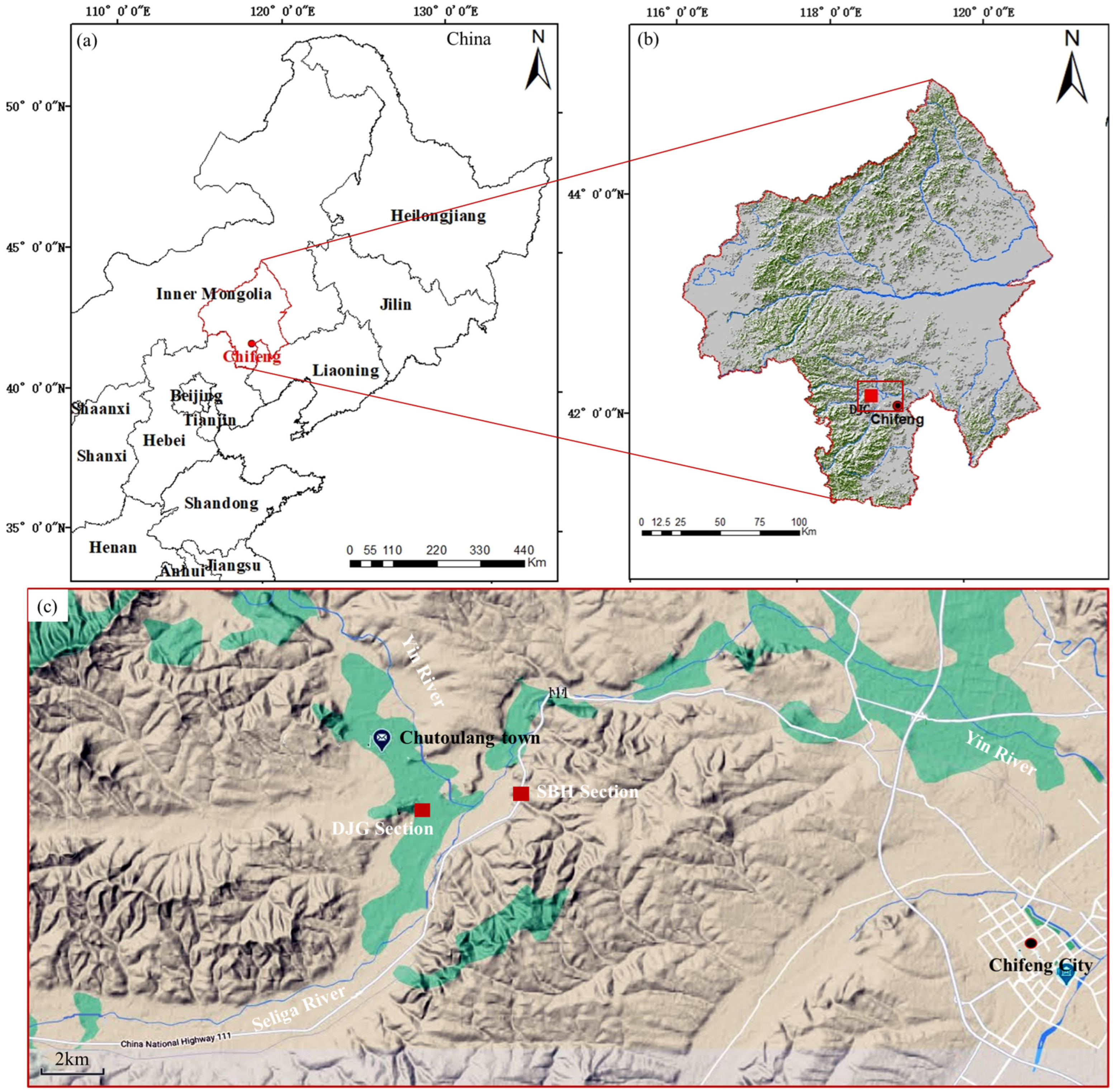
2.1. Study Area and Loess Sections

The study area—where the main landform comprises high elevation in the west and low elevation in the east—is situated in Chifeng, NE China. The region consists of hills and valleys with elevations ranging from 661 to 1384 m (Figure 1) [40]. The loess deposited in this area is mainly Quaternary Aeolian loess [24]. The area has a typical temperate continental monsoon climate influenced by East Asian Monsoon circulation dynamics, where the ranges of mean annual temperature (from 1951 to 2013) and precipitation are 0–7 °C and 300–500 mm, respectively [41].
The DJG loess section (42°18′4″ N, 118°38′34″ E) is exposed on a terrace, where the Yin and the Seliga Rivers meet. The DJG loess section is located in a gully about 2.4 km northwest from the SBH section (42°18′27″ N, 118°41′17″ E) (Figure 1c). The DJG section’s lithology mainly consists of ten pedostratigraphies, including light brown loess layers (L1–2S2 and L1–3S1) interbedded with weakly developed paleosols (L1–1S, L1–2S1, L1–2S3, and L1–3S2), red paleosol layers (S), and loess layers (L1–1L, L1–2L, L1–3L) (Figure 2). According to the field guidelines by Schoeneberger et al. [42], the loess section consists of 20 genetic horizons within 12.32 m depth.

2.2. Soil Sampling and Laboratory Analysis

Approximately 30 cm of the exposed soil surface was removed for describing the soil morphology characteristics (i.e., color, texture, structure, compactness, and horizons) and sampling [43,44,45]. Following the description, pedostratigraphies, genetic horizons, and 5 cm interval soil samples were collected to ascertain various characteristics (i.e., soil age dating, chemical and physical properties, and magnetic susceptibility): (1) a total of 8 optically stimulated luminescence (OSL) samples were collected from the freshly exposed surface located at the pedostratigraphic boundaries using light-avoided steel cylinders with a diameter of 5 cm and a length of 20 cm [46]; (2) 20 genetic horizon samples were collected for physical and chemical analyses; (3) a total of 247 samples were collected at 5 cm intervals from the bottom to the top of the DJG section for measurement of magnetic susceptibility (MS) and grain-size distribution. All soil samples were transported to the laboratory, and the genetic horizon and 5 cm interval samples were air-dried for 7 days. The air-dried samples were cleared of roots and other organic debris. Subsequently, the soil was ground and passed through a 2 mm screen to prepare it for further laboratory analysis.
The MS2 meter was utilized to measure the low-frequency mass MS of 247 samples at a frequency of 470 Hz with an error rate of 1%. The measurements were normalized by mass [47]. Organic matter and carbonates within the soil matrix were removed using the 10% H2O2 and 10% HCl solution, respectively [48]. The grain size was determined using a Malvern 2000 laser diffractometer (Malvern Instruments Ltd., Malvern, UK) [49]. The soil pH was determined potentiometrically at a soil/solution ratio of 1:2.5 using a PHS-3C pH Meter [50]. Soil bulk density was determined by dividing the mass of soil matrix in the cylindrical core by the volume [51]. Soil carbonate concentrations were measured using the modified gas evolution method [52]. The major elemental composition was determined using inductively coupled plasma (ICP) [53].

2.3. OSL Soil Age Dating

2.3.1. Sample Preparation

The OSL samples enclosed in steel tubes were transported to the laboratory under sealed and light-protected conditions. The preprocessing of OSL samples aimed to extract the sedimentary quartz for measurement of the radiation dose and estimating the loess deposition time. The preprocessing steps were conducted in subdued red-light conditions (center wavelength: 655 ± 30 nm) in the laboratory. The unexposed soil samples were weighed around 100 g into the 1000 mL beaker and soaked with distilled water, and 30% H2O2 and 30% HCl were added to remove the organic matter and carbonates, respectively. Then, the soil suspensions were washed and filtered for neutralization with distilled water [54]. Afterward, the fine-sized mixed minerals (diameter: 4–11 μm) were separated from the suspensions according to Stokes’ Law and soaked in fluosilicic acid for about 3 days to exclude feldspar-like minerals to purify fine-grained quartz. Lastly, the purified fine-grained quartz for further measurement can be homogeneously precipitated on stainless steel discs using ethanol [55,56].
After the fine-sized mixed minerals were separated, the residual samples were oven-dried at 40 °C and sieved to extract the coarse-sized mixed minerals with a diameter of 90–125 μm. The feldspar (ρ < 2.62 g/cm3) and heavy minerals (ρ > 2.66 g/cm3) within the coarse-sized mixed minerals were removed using polytungstate solutions. Then, the remaining mineral grains were soaked in a 40% HF solution for 1 h to remove the surface portion of the feldspar and quartz grains affected by α-rays. Later, the samples were soaked in 35% fluorosilicate for about 2–5 days and washed with warm HCl (10%) to remove the precipitated fluorides for purifying quartz grains (90–125 µm). Lastly, the purified quartz grains were fixed in the center area of the 9.7 mm diameter stainless steel discs using silicone oil to determine the equivalent dose (De) [57,58].

2.3.2. De and Dose Rate Determination

The OSL measurements were performed on a Risø TL/OSL-DA-20 reader [59], and the tests were controlled by the sequence (program) set by the computer. The De values of quartz (90–125 μm) were measured using the single-aliquot regenerative-dose (SAR) protocol (Table 1) [55,60]. Different doses produced different OSL signal intensities, which were corrected for susceptibility changes by the test dose. A dose growth curve was established using the corrected OSL signal intensity for each irradiation dose. Then, the corrected natural OSL signal intensity was projected onto the growth curve, and the corresponding equivalent dose was calculated by backward extrapolation.
The De values of purified quartz (4~11 μm) were measured using the simple multiple-aliquot regenerative-dose (SMAR) protocol (Table 1) [54,60]. At the end of the multi-aliquot natural- and regenerative-dose OSL signal (Li) test, all aliquots were irradiated with the measured dose for one hour, and the resulting sensitivity change was monitored and corrected with the measured dose OSL signal (Ti). The equivalent dose value is the ratio of the natural dose to post-test dose OSL signal (Li/Ti) [57].
For all samples, inductively coupled plasma mass spectrometry (ICP-MS) was used to measure the uranium (U) and thorium (Th) concentrations, and K content was determined by inductively coupled plasma optical emission spectrometry (ICP-OES) analysis [58]. The experiment was conducted at the Analysis and Testing Center of the Institute of Earth Environment, Chinese Academy of Sciences.
The environmental dose rates can be calculated using the following equation:
D = 0.04 Dα + Dβ + Dγ + Dc
where D represents environmental dose rates; Dα, Dβ, and Dγ represent the dose rates (Gy/a) from α, β, and γ radiation in the environment. The values of Dα, Dβ, and Dγ were obtained by converting the U, Th, and K concentrations in the samples and correcting for water content [61]. Dc represents the dose rate from cosmic rays.
Following the De and dose rate determination, the ages of OSL samples from the DJG section can be calculated using the following equation:
A = De/D
where A represents the age (in ka); De represents the equivalent dose (in Gy); D represents the environmental dose rate (in Gy/ka).

2.4. Data Analyses

2.4.1. Parent Material Uniformity

Cremeens et al. [62] summarized a mathematical quantitative equation for the uniformity value of the parent material.
U V = [ ( s i + v f s ) / ( s v f s ) ] u p p e r [ ( s i + v f s ) / ( s v f s ) ] a d j a c e n t   l o w e r 1.0
where si represents the silt (2–50 μm) concentration (%); vfs represents the very fine sand (50–100 μm) concentration (%); and s represents the sand (50–2000 μm) concentration (%).

2.4.2. Chronology

Interpolation based on the magnetization model (Equation (3)) was used to reconstruct the paleoclimate [63].
T m = T 0 + T 1 T 0 i = 1 m a i s i i = 1 n a i s i 1
where Tm represents the age of a layer (i); T0 and T1 represent the ages of the two control points; n represents the total number of layers between the two age control points; m represents the total number of layers before the age of the requested layer; ai represents the thickness of a layer; si represents the mass magnetization value of a layer. T0 and T1 can be any point in the section, T1 > T0.

2.4.3. Soil Redness Rating

The redness rating (RR) values can be used to estimate pedogenic strength, which can be computed using Equation (4) [64,65,66].
RR = (K − H) × C/V
where K is 12.5; C represents the chroma; V represents the value; and H is determined according to hue (i.e., 10YR = 10, 7.5YR = 7.5, 5YR = 5, 2.5YR = 2.5).

2.4.4. Soil Chemical Weathering Intensity Index

The elemental molar ratios widely used in loess research include the Chemical Index of Alteration (CIA) [67], K2O/Na2O ratio [68], SiO2/Al2O3 ratio (Sa), Fe2O3/Al2O3 ratio [69], ba value, and Ki value, which were used in this study to quantify the weathering intensity of the DJG section. The measured molar CaO content was corrected for Ca in apatite using the available measured P2O5 content, and the CaO/Na2O molar ratio was assumed to not be greater than that in the silicate material. When the remaining mole of CaO (corrected for apatite) was greater than Na2O, mNa2O was adopted. In contrast, when the remaining mole of CaO was less than that of Na2O, mCaO* was used [14,69].

3. Results

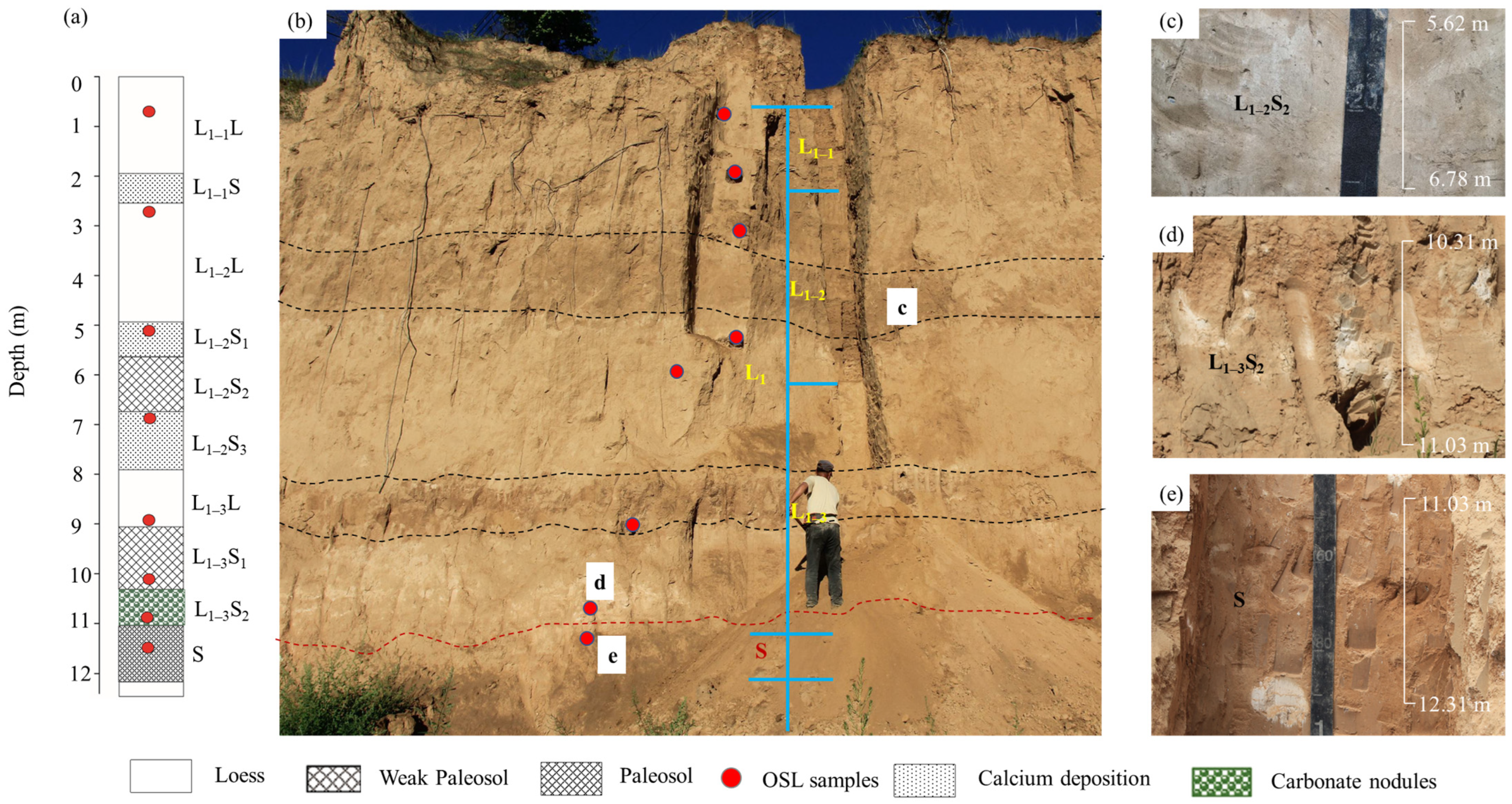
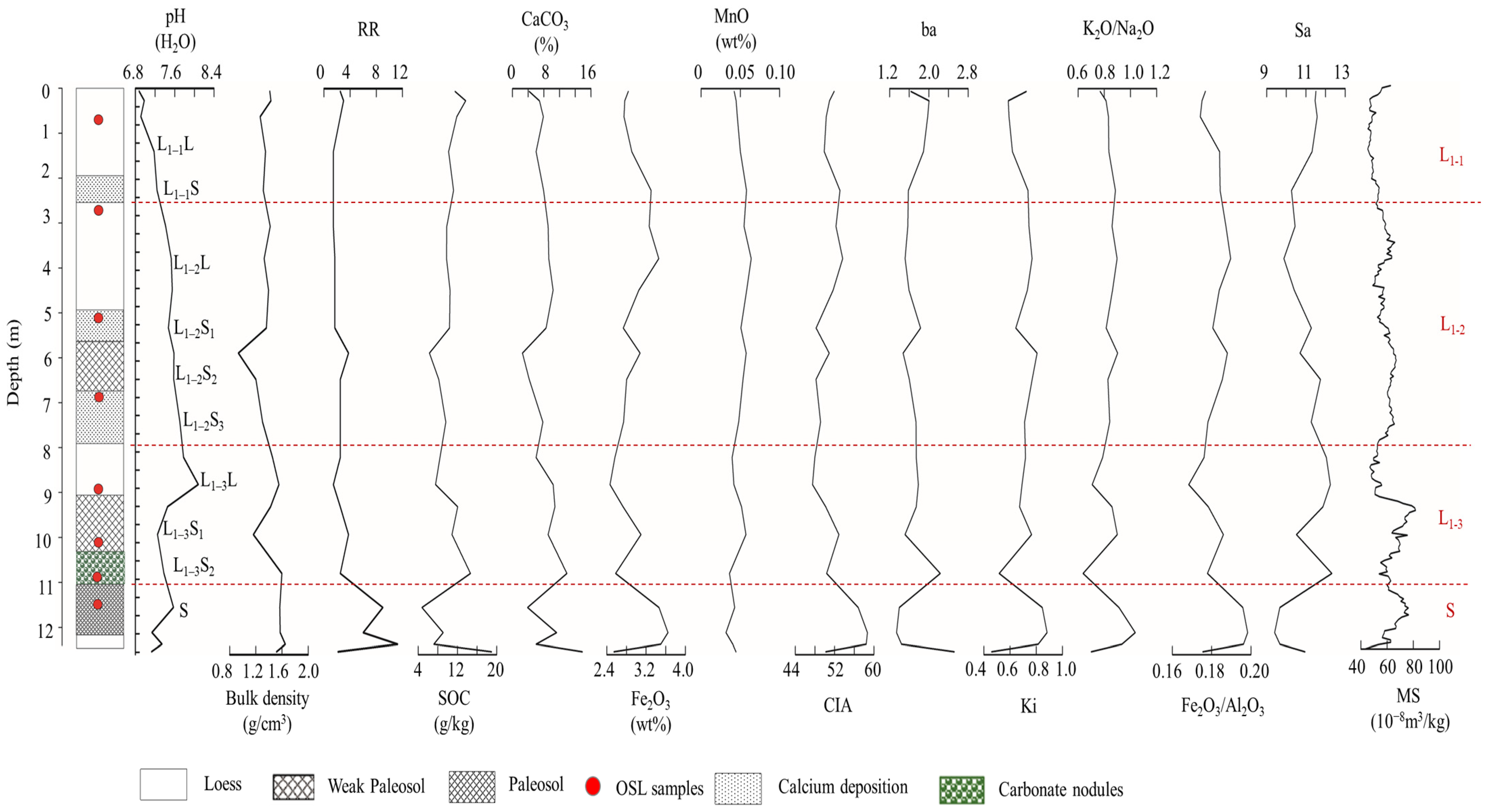
3.1. Soil Morphological Characteristics of the DJG Section

The thickness of the DJG section was 12.32 m. It can be observed that the pedostratigraphy was clear, as shown in Figure 2. The whole section was divided into loess (L1) (0–11.03 m) and red paleosol (11.03–12.32 m) (S). The L1 layer was divided into the pedostratigraphic sub-layers L1–1 (0–2.53 m), L1–2 (2.53–7.90 m), and L1–3 (7.90–11.03 m), each marked with a specific symbol throughout the section (Figure 2a). According to the soil color and calcium carbonate presence (Table 2), the L1–1 layer was divided into L1–1L (0–1.95 m) and L1–1S (1.95–2.53 m); the L1–2 layer was divided into L1–2L (2.53–4.92 m), L1–2S1 (4.92–5.60 m), L1–2S2 (5.60–6.78 m), and L1–2S3 (6.78–7.90 m); and the L1–3 layer was divided into L1–3L (7.90–9.09 m), L1–3S1 (9.09–10.31 m), and L1–3S2 (10.31–11.03 m). Among the layers, the L1–1S, L1–2S1, and L1–2S3 layers had different degrees of calcium carbonate accumulation; the L1–3S2 layer formed calcium carbonate nodules of different sizes. In addition, the L1–2S2 and L1–3S1 layers were brown (10YR 4/4), and the S layer was red (i.e., a paleosol layer).

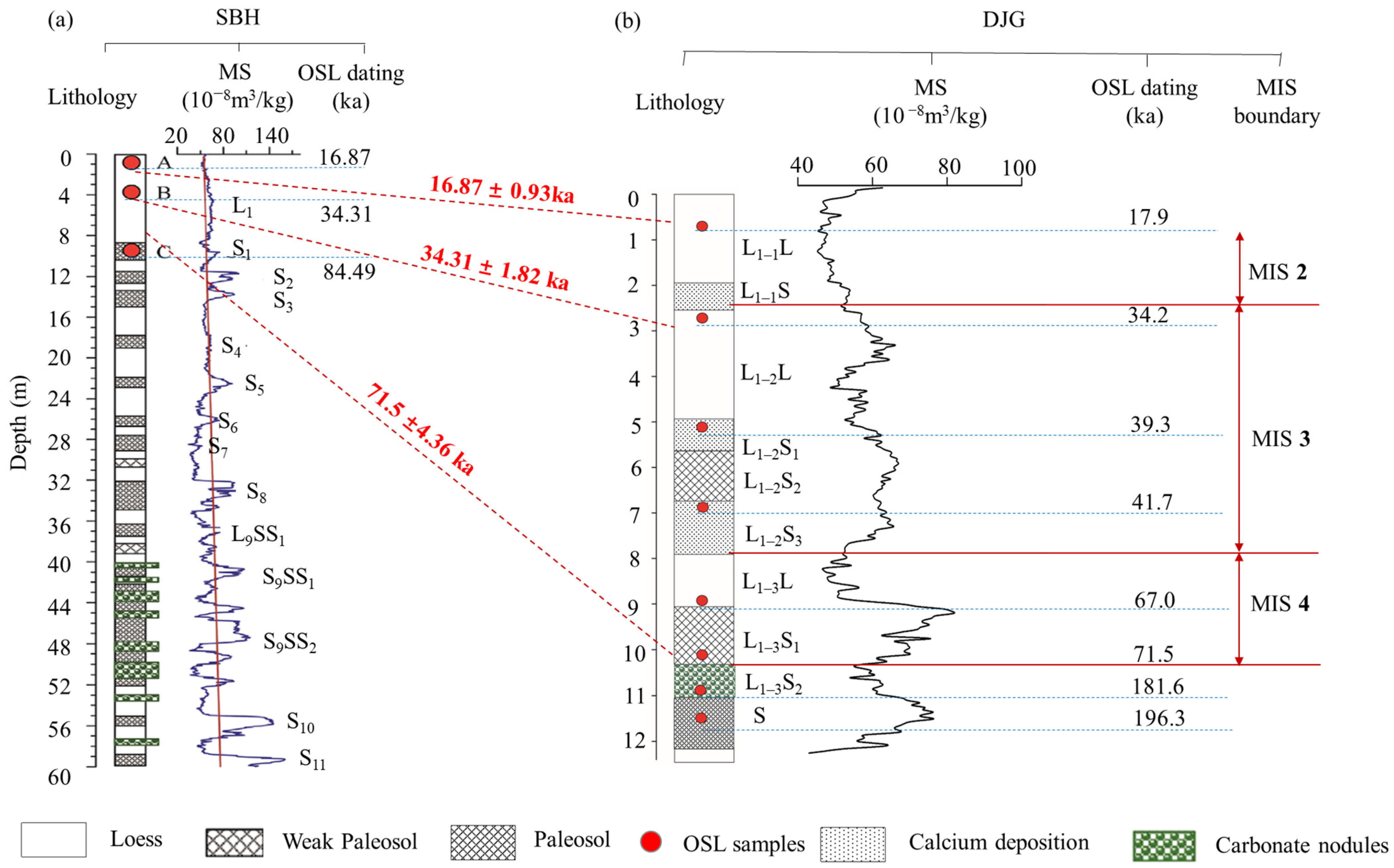
3.2. Sedimentary Characteristics and Age of the DJG Section

3.2.1. Soil Age of the DJG Section

Depositional age determination of the DJG section was conducted at the Analysis and Testing Center of the Institute of Earth Environment, Chinese Academy of Sciences (Table 3). The De values range from 71.14 ± 2.65 Gy to 721.95 ± 15.48 Gy from the upper layer to the sub-layer. Correspondingly, the soil age of the upper layer is 17.94 ± 1.14 ka, and the soil age of the sub-layer is 196.34 ± 10.89 ka. The depositional ages of upper L1–1L (0.6 m), upper L1–2L (2.76 m), upper L1–2S1 (5.05 m), upper L1–2S3 (6.63 m), lower L1–3L (9.0 m), lower L1–3S1 (10.31 m), lower L1–3S2 (11.03 m), and middle S (11.31 m) were 17.94 ± 2.65, 34.27 ± 2.50, 39.27 ± 2.79, 41.67 ± 1.61, 66.97 ± 4.72, 71.50 ± 4.36, 181.58 ± 10.42, and 196.34 ± 10.89 ka, respectively (Table 3). The age of sample 6—collected at a depth of 10.31 m from the bottom of the L1–3S1 layer—was 71.5 ± 4.36 ka (De = 277.26 ± 4.92 Gy), which was in agreement with the age (71 ka) of L1/S1 boundary within the margin of error [4]. Several papers had suggested that a reliable quartz OSL De value for loess distributed in China is around ~230 Gy (or lower than 300 Gy) and that the saturation age is around ~100 ka [9,57,58]. Two quartz samples—L1–3S2 and middle S—have De values higher than 300 Gy. The reliability of these two layers could not be confirmed in this study; therefore, all layers above the L1–3S2 layer (depositional age at 71.5 ± 4.36 ka) were studied. The ages of all samples, except those from the L1–3S2 and S layers, were close to expected values. The chronology of the DJG section was generated via linear interpolation of the MS model (Equation (4)).

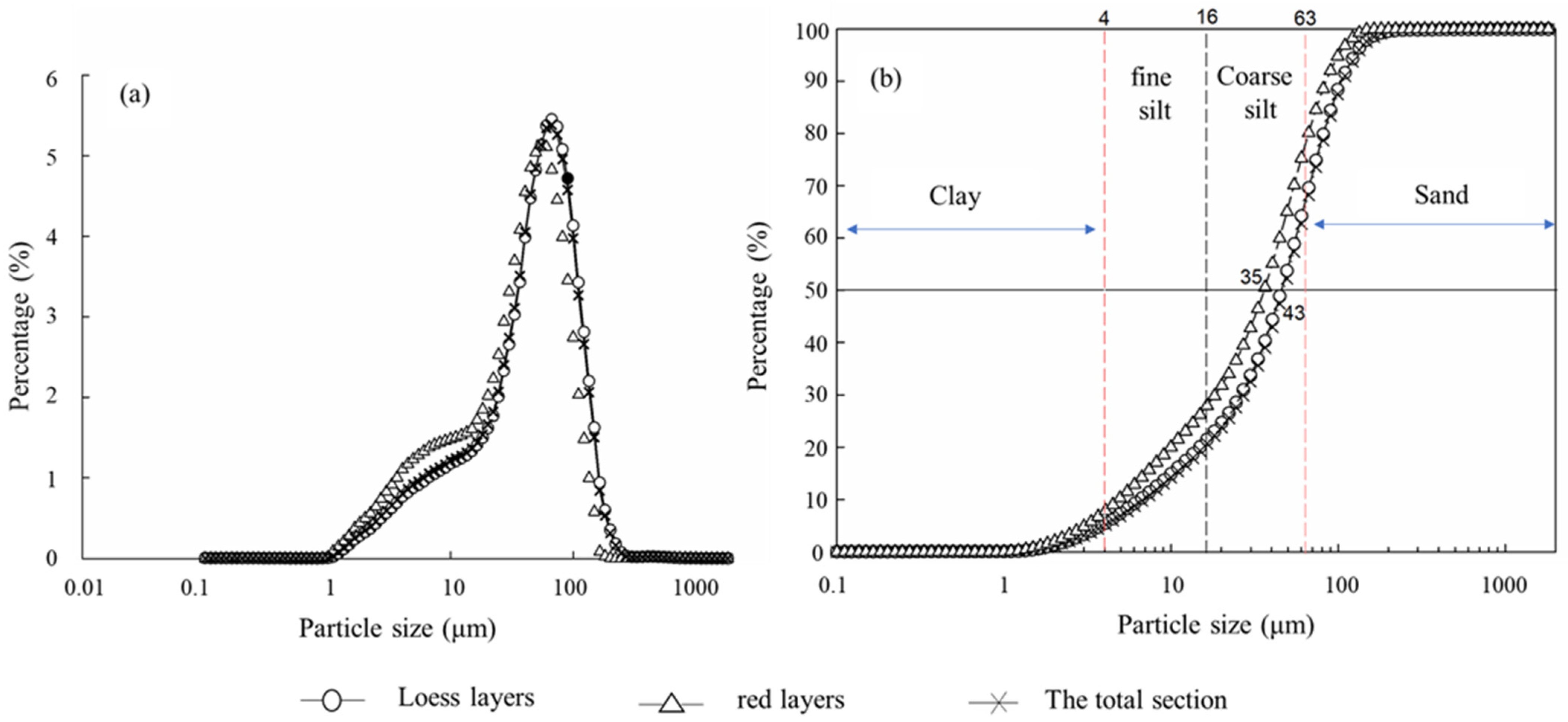
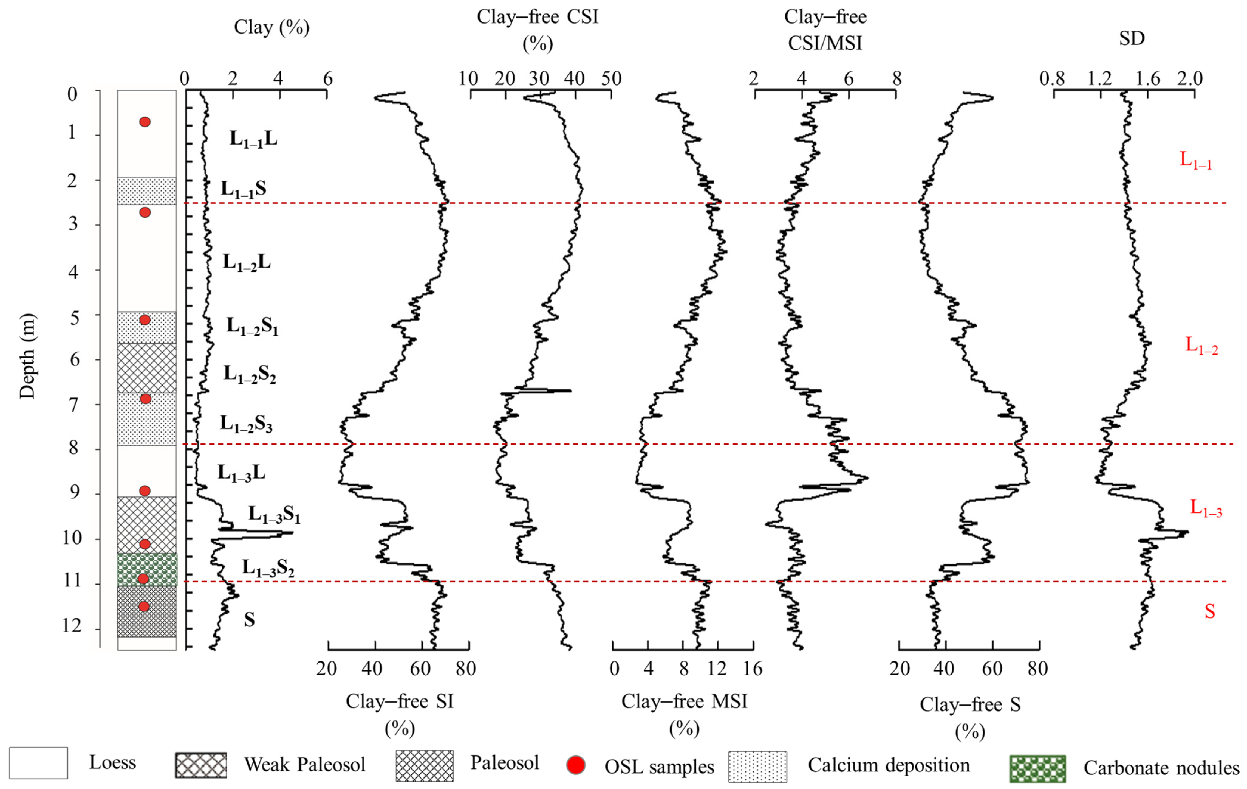
3.2.2. Grain-Size Characteristics

The frequency curve of the DJG section showed a bi-modal distribution (Figure 3a), with the greatest peak at 30–70 μm—accounting for ~55% of the soil by weight relative to the basic dust fraction [20]—and a low peak at 5–10 μm. The ratio (%) reached a maximum mode size and decreased in both coarse and fine directions, with a long tail on the fine side, which was skewed toward the coarser side and was thus asymmetric. The cumulative curve of the DJG section (Figure 3b) was S-shaped, with straight line as the main body, and the samples comprised a coarse component (30–80%) with a modal size range of 35–43 μm. The cumulative curve of the DJG section contained inflection points at 3 and 9 Φ.
Considering the particle-size distribution of the DJG sections (Figure 4), the clay, silt, and sand fractions varied with depth and were mainly related to pedogenesis processes and the original deposition of eolian loess, as reported in a previous work [39]. The clay concentration in the L1–1 layer was <1%, and the silt (50–2 μm particle size) concentration increased to a maximum of 70% in the L1–1S layer; conversely, the sand concentration decreased to 29%, with little change in standard deviation (SD) in the vertical direction (Figure 4). The clay concentration in the L1–2 layer was <1%; the silt concentration decreased to a minimum of 29% in the L1–2S3 layer; meanwhile, the sand concentration reached 70%, with little change in SD. The clay concentration in the L1–3 layer first increased to 4% with depth in the L1–3S1 layer, then decreased to 1% in the L1–3S2 layer. The silt concentration gradually increased from 27% in the L1–3L layer to about 50% in the L1–3S1 layer. The sand concentration gradually decreased from 70% in the L1–3L layer to about 50% in the L1–3S1 layer. The SD at the interface of the L1–3S1 and L1–3S2 layers sharply increased to 2.0, and the SD of the L1–3S2 layer was 1.4. The clay concentration in the S layer was 2%, and the silt concentration was ~70%, with a stable SD of 1.4. The distribution of individual silt fractions on a clay-free basis was 28% for silt particles of 50–2 μm in the L1–2S3 and L1–3L layers and up to 70% for the sand (≥50 μm) concentration in the L1–2S3 and L1–3L layers, which was numerically greater than in all other layers. Apart from the L1–2S3 and L1–3L layers, the concentration of silt particles (50–2 μm) was up to 60% in the remaining horizons, and the coefficient of variation (CV) of the silt concentration was 24 (Table 4). This suggested that the DJG loess section had a uniform source or parent material and a stable depositional environment. The coarse silt (CSI)/medium silt (MSI) ratios of the DJG section ranged from 3 to 6 with a CV of 17 (Table 4).

3.2.3. Parent Material Uniformity of the DJG Section

The UV parameter (Equation (3)) and Ti/Zr ratio indicated uniformity of the sediment source [62,70]. Chen [71] reported that the UV tends to be 0, and the similarity of a parent material source is greater in two layers when the absolute UV is >0.6, indicating different parent materials in adjacent layers. The UVs of the DJG section were <0.6 in each layer (Table 4), indicating that the parent materials were uniform. Drees and Wilding [68] reported that a CV of the Ti/Zr ratio > 22% indicates non-uniform parent materials. In contrast, Chapman and Horn [72] reported that differences > 100% were required to detect lithologic changes. A CV of 15.82% for the Ti/Zr ratio suggested uniform materials throughout the DJG section. These results indicated that the parent material in the DJG section was uniform.

3.3. Soil Pedogenesis Characteristics

Soil bulk density, pH, CaCO3 concentration, RR value, and weathering index changed with depth for the DJG loess section (Figure 5). The bulk density and CaCO3 concentration in the L1–1 layer were ~1.4 g/cm3 and 8%, respectively. The RR value (Equation (5)) and soil organic carbon (SOC) concentration in the L1–1 layer were ~2 and 10 g/kg, respectively. Soil pH increased with depth and ranged from 6.8 to 7.2. The MS was ~50 (10−8 m3/kg). The K2O/Na2O and Fe2O3/Al2O3 ratios were 0.8 and 0.18, respectively. The CIA value was 49 in the lower part of the L1–1L layer and 52 in the L1–1S layer. The (Al2O3 + Fe2O3)/(CaO + MgO + Na2O) value (Ki) increased numerically with depth, and the L1–1S layer had a large Ki value due to calcium accumulation. The SiO2/Al2O3 ratio (Sa) and (CaO + K2O + Na2O + MgO)/Al2O3 (ba) values gradually decreased numerically with depth, and the Sa and ba values were lowest in the L1–1S layer.
Soil bulk density of the L1–2 layer was a minimum of 0.81 g/cm3 in the L1–2S2 layer and remained at ~1.4 g/cm3 in the remaining layers. The SOC and CaCO3 concentrations were low in the L1–2S2 layer—6 g/kg and 2%, respectively—with little variation in the other layers. Soil pH increased from 7.4 to 7.8 with depth. The RR value and Fe2O3 and MnO concentrations in the L1–2S2 layer increased with depth—4, 3.0 wt%, 0.05 wt%, respectively—compared to the adjacent layer (L1–2S1 and L1–2S3 layers). The Fe2O3 concentration was maximum in the L1–2L layer (3.4 wt%), whereas the Sa ratio had a nadir of 9.5, which corresponded to the peak in the MS curve. The CIA and Ki values, as well as the K2O/Na2O and Fe2O3/Al2O3 ratios, were 52, 0.6, 0.9, and 0.19, respectively, whereas the ba and Sa ratios were 2 and 11, respectively, in the L1–2S2 layer.
Soil bulk density in the L1–3L, L1–3S1, and L1–3S2 layers was 1.5, 1.2, and 1.6 g/cm3, respectively. Soil pH in the L1–3L layer reached maximum at 8.0, and it was 7.2 in all other layers. The RR value and Fe2O3 and MnO concentrations in the L1–3S1 layer were 4, 3.2, and 0.05 wt%, respectively. The SOC and CaCO3 concentrations in the L1–3S1 layer were 11 g/kg and 8%, respectively. The CIA and Ki values, as well as the K2O/Na2O and Fe2O3/Al2O3 ratios in the L1–3S1 layer were 54, 0.8, 0.9, and 0.19, respectively, indicating a sharp increase corresponding to the peaks in the MS curve. The ba and Sa ratios were 1.4 and 10, respectively.
Soil bulk density in the S layer was 1.6 g/cm3, and soil pH decreased from 7.4 to 6.9 with depth. The RR value and Fe2O3 concentrations ranged from 8 to 12 and from 3.2 to 3.6 wt%, respectively. The SOC and CaCO3 concentrations were ~6 g/kg and ~4%, respectively. The S layer had the largest CIA and Ki values—as well as K2O/Na2O and Fe2O3/Al2O3 ratios—and the lowest ba and Sa ratios compared to the upper L1 layer in the DJG loess section.

4. Discussion

4.1. Integrating a Typical Loess Section in NE China

4.1.1. Feasibility of Integrating Typical Sections

Full comparison of the sediment types, genesis processes, deposition ages, and geomorphic features of DJG and SBH sections is a prerequisite for integration. The DJG and SBH sections were derived from aeolian loess, which indicated the feasibility of integrating these two sections for paleoclimate reconstruction [27,41]. This inference was reasonable, given the bi-modal distribution of the frequency curve of grain-size distribution in the DJG section (Figure 3a). Bi-modal distribution is consistent with the loess found on the Loess Plateau in China [73], which also has a bi-modal distribution with overlapping coarse and fine grains—the main component of coarser grains. It has pronounced kurtosis and good sorting, which varies depending on the ratios of the two components and mode size. Furthermore, the greatest peak domain of the 30–70 μm coarse particles—accounting for ~55% of the soil by weight—indicated typical loess, and thus, an eolian origin [73]. The eolian particle dynamics indicated that the coarse-grain fraction was generally transported by surface winds over a short distance [74]. The cumulative curve of the grain-size distribution (Figure 3b) was S-shaped, with straight line as the main body of the curve, and contained 3 and 9 Φ inflection points. The size of grains transported in low-altitude suspended dust is >4–6 Φ or 4.3 Φ, whereas those <4.3 Φ on the ground are transported by being rolled or bounced (i.e., saltation) [75,76]. These results support the conclusion that the DJG section contained typical aeolian loess and that the transport mode of the DJG section was mainly low-altitude suspension, with a small portion of particles being transported by saltation.
A comparison of MS curve variations between the two loess sections indicated that the L1 layer of the SBH section had no shifts with depth, whereas the DJG section varied with depth (Figure 6). The MS curve of the loess sequence reflects multi-cycle variations in the paleoclimate and can be compared with marine oxygen isotope records [4,77], further indicating that the DJG section contains multiple alternating cold–dry and warm–wet stages due to differences in pedogenesis [78]. A comparison of the color, geochemical indices, and soil weathering index variability provided additional support for the DJG section having undergone different pedogenic intensities.
Soil color is the most visual representation of soil properties, and changes in loess soil color are caused by local climatic conditions, strong or weak weathering and pedogenesis, and corresponding changes in the original composition [22,66]. The RR value represents the reddening process of the soil during pedogenesis and closely correlates with large and small lithostratigraphic values in paleosols and loess units, respectively [65]. The RR value of the L1–2S2, L1–3S1, and S layers was large in the DJG section, implying stronger pedogenesis than in the adjacent layers (Figure 5). The low calcium carbonate concentration in the L1–2S2, L1–3S1, and S layers indicated that decalcification had occurred. Geochemical indices indicated initial weathering and pedogenesis [79]. The degree of weathering was identified in the DJG section using the soil weathering index (Figure 5). The CIA can indicate pedogenesis and weathering. Fedo et al. [80] classified the degree of soil weathering based on CIA values of 50–60, 60–80, and >80 as primary, intermediate, and extreme, respectively. The CIA values of the L1 layer were <55 (Figure 5), indicating that the layer was likely unweathered. The L1–3L layer had the lowest CIA value, indicating the weakest weathering in the entire section. The S layer had a CIA value of 60, indicating a primary degree of weathering. The CIA values of the L1–2S2, L1–3S1, and S layers were larger compared to the adjacent layers in the DJG section, implying a higher degree of soil weathering than in the adjacent layers.
Because a relatively large carbonate concentration might impact the absolute chemical composition of loess owing to various degrees of leaching and illuviation during soil formation, element ratios are used to minimize the effect of carbonate dilution and infer past climate variation [81]. Liu [20] proposed that the Sa ratio gradually decreases with increased soil weathering, whereas the K2O/Na2O ratio tends to increase during soil formation. The Sa and K2O/Na2O ratios gradually decreased and increased, respectively, in the L1–2S2, L1–3S1, and S layers (Figure 5) due to different weathering intensities of soil formation. Li et al. [82] proposed that the ba value could reflect the leaching and migration of elements Ca and Na, whereas the Ki values could reflect the relative enrichment of Fe and Al. The large Ki values—as well as K2O/Na2O and Fe2O3/Al2O3 ratios—in the L1–2S2, L1–3S1, and S layers and the low ba values indicated enrichment of Fe and Al and leached Ca and Na due to strong weathering. The L1–2S2, L1–3S1, and S layers of the DJG section had numerically greater RR values, leached Ca and Na, and enriched Fe and Al caused by stronger pedogenesis compared to the L1 layer in the SBH section. Thus, the DJG section had undergone different pedogenic intensities and recorded multi-cycle variations in the paleoclimate. Consequently, the DJG section can be integrated with the upper part (i.e., the L1 layer) of the SBH section to overcome the missing paleoclimatic information in the SBH section.

4.1.2. Outcome of Integrating Two Typical Loess Sections

The lithostratigraphic comparison in the field and the depositional ages of the two sections showed that the L1 layer of the DJG section (i.e., 10.31 m, 71.5 ka) could be integrated with the upper part (i.e., the L1 layer) of the SBH section (Figure 6). The isochrons between the two sections were established based on the reliable independent chronology of these two sections (Figure 6) [83].
The upper part of the L1–3S1 layer (10.31 m) was selected for integration because the L1–3S1 layer has continuous deposition, whereas the lower L1–3S1 layer has intermittent deposition. The deposited ages of the L1–3S1 and L1–3S2 layers were ~71.5 and ~181.58 ka, respectively. The deposited age of the L1–3S2 layer (i.e., with carbonate nodules) ranged from 181 ± 10.42 to 71.5 ± 4.36 ka. Depositional interruptions might be caused by erosion between depositional events, as one layer does not reflect climate changes over hundreds of thousands of years [84].
The SD of all particles in the DJG section provided additional support for the loess deposit being discontinuous, where the SD is often used to indicate uniformity of the sediment and distinguish the sedimentary environment [85,86]. Based on the large fluctuations in the SD of all particle sizes in the L1–3 layer of the DJG section, the DJG section was considered interrupted in the lower part of the L1–3 layer. This inference was reasonable, given that the SD was minimal in the upper part of the L1–3 layer (SD = 1.2), indicating good sorting. However, the SD sharply increased to 2.0 at the interface of the L1–3S1 and L1–3S2 layers, indicating poor sorting (Figure 4). The field investigation revealed a fine sand and gravel layer at the interface of the L1–3S1 and L1–3S2 layers, which might have been influenced by flowing water. Therefore, the interface of L1–3S1 and L1–3S2 layers might have experienced intermittent deposition. Moreover, the soil age in the lower part of the L1–3S1 layer was 71.5 ka; hence, the deposition was continuous until 71.5 ka and intermittent after 71.5 ka. The upper part of the L1–3S1 layer (10.31 m) was selected for integration with the SBH section deposited 71 ka ago. As the deposition of the DJG section was discontinuous during 84 ka–71 ka, another section should be integrated with the SBH section, so that a continuous record can be obtained from 1.22 Ma. However, the deposition of the DJG section has been continuous since 71 ka and intermittent after 71 ka; hence, 71 ka was selected for paleoclimate reconstruction and interpretation.

4.1.3. The Advantages and Limitations of Integrating the Loess Sections

Integrating the target sections of loess could reconstruct regional long-term continuous paleoclimate records where discontinuous loess sequences occurred. In addition, integrating the target sections of a region would render the study more purposeful and save a great amount of time and labor. Based on the integrated loess section, paleoclimate records can be rapidly and accurately reconstructed using soil age dating methods. However, a full comparison of the sediments, genesis processes, and geomorphologies of these sections is needed before integration, which requires detailed investigations and data as supports. The problem of homogeneity arises during the integration of sections. For example, the integration parts of the two sections may have the same depositional age but different genesis. The integration part may have the same depositional age, but the parent material may not be uniform. The depositional ages, genesis processes, parent materials must be the same for the junction layers of the integration sections, which are very difficult to find. These integration prerequisites restrict the wide use of integration. Another problem is that sampled sections may also experience depositional discontinuity events, and only the depositional continuum layer would be integrated with the target section. The discontinuous depositional layer of the section should find another section for integration with the target section in order to reconstruct a continuous and complete record.

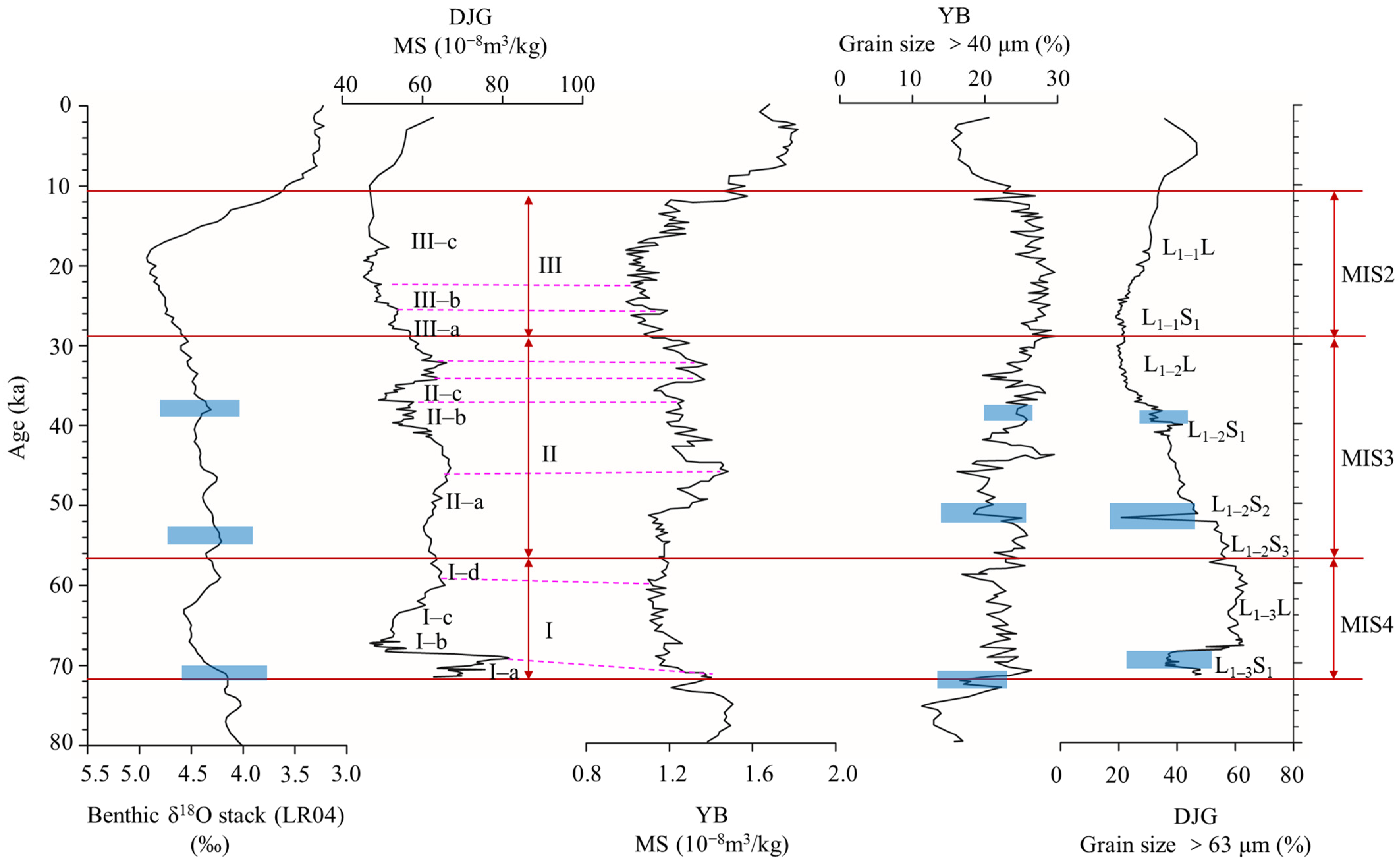
4.2. Reconstructing the Paleoclimate of NE China

The MS curve of the loess–paleosol sequence reflects multi-cycle variations in the paleoclimate and can be compared with the marine oxygen isotope record [4,34,87]. Grain size is a good proxy for the Asian winter monsoon [6,30,88]. During dust transportation, wind sorting is an important factor in the abrasion and size reduction of dust particles [89]. In this study, the climate change information in NE China was interpreted based on the MS and content of the coarse fraction > 63 μm (Figure 7). The perpendicular direction of the coarse fraction content > 63 μm represents the direction of dust transport, which corresponds to that of regional wind [90].
According to the marine isotope stage (MIS) boundary, the MIS 1/2, MIS 2/3, MIS 3/4, MIS 4/5, and LR04 ages were 11.7, 29, 57, and 71 ka, respectively [91]. The climatic evolution of the last glacial period in the DJG section can be divided into three large zones and ten sub-zones (Figure 7). The paleoclimate of NE China was generally divided into stages I, II, and III (Table 5). The climate changed from warm and humid to cold and dry from 71 to 57 ka during stage I (equivalent to MIS 4), alternated between cold and warm temperatures from 57 to 29 ka in stage II (equivalent to MIS 3), and was overall cold and dry from 29 to 11.7 ka but warm from 18 to 11.7 ka in stage III (equivalent to MIS 2) (Figure 7 and Table 5). The substantial strengthening of the winter monsoon around 39, 52, 56, and 62 ka was almost synchronous with the occurrence of the Heinrich event [92].
In MIS 4, the MS curve fluctuation trend of the DJG section showed that the climate changed from warm to cold, which coincided with the gradually increasing ice volume in the benthic δ18O curve (Figure 7) [93]. In MIS 3 (i.e., 57–29 ka), the climate recorded in the DJG section was unstable and fluctuated significantly (alternating between warm and cold), which was consistent with the unstable climate recorded by the benthic δ18O curve. In MIS 2 (i.e., 29–11.7 ka), the cooling–drying trends recorded in the DJG loess section were correlated with the increase in high-latitude ice volume. This is consistent with the hypothesis that cooling and ice volume expansion at high latitudes were the drivers of long-term stepwise aridification of the Asian interior [1,26,94] (Figure 7).
In this study, the Yuanbao (YB) section of the CLP was selected for comparison with the DJG section (Figure 7). Chen et al. [95] pointed out that the YB section—located at the northwestern edge of the CLP—was a representative eolian loess depositional section, with the Malan loess layer (i.e., layer L1) containing nine pedogenic layers. The results indicated that the YB section recorded a high-resolution history of summer and winter monsoon climate variations over the last 75 ka, which showed a high degree of similarity with the warm interstadials recorded in ice cores from Greenland and the Antarctic. Variation in the MS curve of the DJG section coincided well with the MS curve of the YB section, indicating that the fluctuations in paleoclimate were consistent (Figure 7). During MIS 2, both DJG and YB sections recorded a generally weak summer monsoon (low MS values), while the winter monsoon was quite strong and variable, which coincided with cold global temperatures. During MIS 3, in the DJG and YB sections, the MS curves showed a similar pattern of variation, and the main MS peaks could be easily correlated between the two sections. Chen et al. [95] showed that the summer monsoon was generally very strong and variable, while the winter monsoon was quite weak during 50–30 ka. However, upon detailed comparison, the paleoclimate information reflected by the DJG section was not a one-to-one correspondence with the YB section. The differences may be the result of regional climatic effects and a relatively high degree of variability in the depositional environment over short distances [96]. During MIS 4, the climate recorded in the DJG section changed from warm and humid to cold and dry. Chen et al. [95] indicated that the summer monsoon was generally weak and showed a small range of variation, but in addition, the winter monsoon was not strong and did not show a range of variation during 70–50 ka. There were some differences in the start and end times of the warm period, which might have been due to the different dating methods.
Variations in grain-size distribution coincide well with loess and pedogenic layers (Figure 7). The percentage of coarse fraction can indicate variability in the Asian winter monsoon [88]. Several times, the content of coarse fraction in the DJG and YB sections decreased significantly, which corresponded to warm periods in the benthic δ18O curve (Figure 7). The grain-size distribution curves (>40 μm) from the YB section displayed a high-frequency, high-amplitude pattern, while the DJG section had relatively low amplitudes. Moreover, it is noteworthy that the grain-size distribution of the DJG section was overall coarser than the YB section, which might have been caused by topographic variation and by the distance to dust sources [96]. Overall, the paleoclimate record preserved by the DJG section was consistent with that preserved by the benthic δ18O curve and the YB section, demonstrating that the chronology of the DJG section was valid and could be used for paleoclimate reconstruction in NE China.
Figure 7. Comparisons of MS, fraction of grain size > 63 μm of the DJG section with the benthic δ18O stack (LR 04) [93], and the YB section [95]. MS represents magnetic susceptibility; Md represents median grain size; and the DJG and YB sections represent the Dajiugang and Yuanbao sections, respectively. The red lines represent the boundaries of the MIS stages. The pink dotted lines indicate MS peaks of the DJG section, corresponding to MS peaks of the YB section. The blue squares show the warm periods in the DJG and YB sections, which correspond to the benthic δ18O stack.
Quaternary 07 00007 g007

5. Conclusions

This study showed that the DJG section could be merged with the upper part (layer L1) of the target SBH section. The DJG section was close in proximity to the SBH section, and the parent material and genesis of these two sections were similar, with clear and identical depositional ages. In particular, the DJG section recorded multiple climate cycles and could overcome the lack of paleoclimatic information in the SBH section from 71 ka. The paleoclimate record preserved by the DJG section was consistent with the benthic δ18O stack (LR 04) and the YB section. The overall climate of NE China during 29–11.7, 57–29, and 71–57 ka was cold and dry, alternately cold and warm, and warm and wet to cold and dry, respectively. The paleoclimate information of the target SBH section during 84–71 ka will need to be integrated with another loess section because the DJG section was discontinuous during 181–71 ka. Integrating the target sections could be an alternative method of reconstructing long-term continuous paleoclimate records.

Author Contributions

Conceptualization, Q.-B.W. and J.L.; methodology, J.L. and M.-G.Z.; software, J.L.; validation, J.L., Z.-D.J. and Q.-B.W.; formal analysis, J.L.; investigation, J.L., T.-H.W., M.-G.Z., Z.-D.J. and Z.-X.S.; data curation, J.L.; writing—original draft preparation, J.L.; writing—review and editing, J.L., K.R.B., Z.-D.J., Z.-X.S., P.R.O., T.-H.W. and Q.-B.W.; funding acquisition, Q.-B.W. All authors have read and agreed to the published version of the manuscript.

Funding

This work was supported by the National Natural Science Foundation of China (No. 41771245).

Data Availability Statement

The data presented in this study are available on request from the corresponding author. The data are not publicly available due to privacy.

Acknowledgments

The authors sincerely thank Hong-Yu Gu and Si Chen for their help in soil sampling and laboratory analysis.

Conflicts of Interest

The authors declare no conflicts of interest.

References

  1. Ding, Z.L.; Derbyshire, E.; Yang, S.L.; Yu, Z.W.; Xiong, S.F.; Liu, T.S. Stacked 2.6-Ma grain size record from the Chinese loess based on five sections and correlation with the deep-sea δ18O record. Paleoceanography 2002, 17, 5–21. [Google Scholar] [CrossRef]
  2. Obreht, I.; Zeeden, C.; Hambach, U.; Veres, D.; Marković, S.B.; Bösken, J.; Bačević, N.; Gavrilov, M.B.; Lehmkuhl, F. Tracing the influence of Mediterranean climate on Southeastern Europe during the past 350,000 years. Sci. Rep. 2016, 6, 36334. [Google Scholar] [CrossRef]
  3. Liu, T.S.; Ding, Z.L. Chinese loess and the paleomonsoon. Annu. Rev. Earth Planet 1998, 26, 111–145. [Google Scholar] [CrossRef]
  4. An, Z.S.; Kukla, G.J.; Porter, S.C.; Xiao, J.L. Magnetic susceptibility evidence of monsoon variation on the Loess Plateau of central China during the last 130,000 years. Quat. Res. 1991, 36, 29–36. [Google Scholar] [CrossRef]
  5. Anwar, T.; Kravchinsky, V.A.; Zhang, R.; Koukhar, L.P.; Yang, L.; Yue, L. Holocene climatic evolution at the Chinese Loess Plateau: Testing sensitivity to the global warming-cooling events. J. Asian Earth Sci. 2018, 166, 223–232. [Google Scholar] [CrossRef]
  6. Guo, F.; Clemens, S.C.; Wang, T.; Wang, Y.; Liu, Y.; Wu, F.; Liu, X.; Jin, Z.; Sun, Y. Monsoon variations inferred from high-resolution geochemical records of the Linxia loess/paleosol sequence, western Chinese Loess Plateau. Catena 2021, 198, 2–11. [Google Scholar] [CrossRef]
  7. Buggle, B.; Hambach, U.; Glaser, B.; Gerasimenko, N.; Marković, S.; Glaser, I.; Zöller, L. Stratigraphy, and spatial and temporal paleoclimatic trends in Southeastern/Eastern European loess–paleosol sequences. Quat. Int. 2009, 196, 86–106. [Google Scholar] [CrossRef]
  8. Haase, D.; Fink, J.; Haase, G.; Ruske, R.; Pécsi, M.; Richter, H.; Altermann, M.; Jäger, K.D. Loess in Europe—Its spatial distribution based on a European Loess Map, scale 1:2,500,000. Quat. Sci. Rev. 2007, 26, 1301–1312. [Google Scholar] [CrossRef]
  9. Panin, P.G.; Filippova, K.G.; Bukhonov, A.V.; Karpukhina, N.V.; Ruchkin, M.V. High-resolution analysis of the Likhvin loess-paleosol sequence (the central part of the East European plain, Russia). Catena 2021, 205, 105445. [Google Scholar] [CrossRef]
  10. Velichko, A.A. Loess-paleosol formation on the Russian plain. Quat. Int. 1990, 7/8, 103–114. [Google Scholar] [CrossRef]
  11. Hall, R.D.; Anderson, A.K. Comparative soil development of Quaternary paleosols of the central United States. Palaeogeogr. Palaeoclimatol. Palaeoecol. 2000, 158, 109–145. [Google Scholar] [CrossRef]
  12. Plata, J.M.; Rodríguez, R.; Preusser, F.; Boixadera, J.; Balash, J.C.; Antúnez, M.; Poch, R.M. Red soils in loess deposits of the Eastern Ebro Valley. Catena 2021, 204, 105430. [Google Scholar] [CrossRef]
  13. Heller, F.; Liu, T.S. Palaeoclimatic and sedimentary history from magnetic susceptibility of loess in China. Geophys. Res. Lett. 1986, 13, 1169–1172. [Google Scholar] [CrossRef]
  14. Sun, Z.X.; Jiang, Y.Y.; Wang, Q.B.; Owens, P.R. Geochemical characterization of the loess-paleosol sequence in northeast China. Geoderma 2018, 321, 127–140. [Google Scholar] [CrossRef]
  15. Gebrechorkos, S.H.; Hülsmann, S.; Bernhofer, C. Statistically downscaled climate dataset for East Africa. Sci. Data 2019, 6, 31. [Google Scholar] [CrossRef]
  16. Xie, S.P.; Vecchi, G.A.; Collins, M.; Delworth, T.L.; Hall, A.; Hawkins, E.; Johnson, N.C.; Cassou, C.; Giannini, A.; Watanabe, M. Towards predictive understanding of regional climate change. Nat. Clim. Change 2015, 5, 921–930. [Google Scholar] [CrossRef]
  17. Sun, Y.B.; Wang, X.L.; Liu, Q.S.; Clemens, S.C. Impacts of post-depositional processes on rapid monsoon signals recorded by the last glacial loess deposits of northern China. Earth Planet. Sci. Lett. 2010, 289, 171–179. [Google Scholar] [CrossRef]
  18. Dodonov, A.E.; Zhou, L.P. Loess deposition in Asia: Its initiation and development before and during the Quaternary. Episodes 2008, 31, 222–225. [Google Scholar] [CrossRef]
  19. Li, Y.; He, S.; Peng, J.; Xu, Q.; Aydin, A.; Xu, Y. Loess geology and surface processes: An introductory note. J. Asian Earth Sci. 2020, 200, 104477. [Google Scholar] [CrossRef]
  20. Liu, T.S. Loess and Environment; Science Press: Beijing, China, 1985. (In Chinese) [Google Scholar]
  21. Chen, Y.M.; Gong, H.L. Study on Loess Records of Climatic Instability during Last Glacial Period; China Environmental Science Press: Beijing, China, 2007. (In Chinese) [Google Scholar]
  22. Hu, X.F.; Wei, J.; Du, Y.; Xu, L.F.; Wang, H.B.; Zhang, G.L.; Wei, Y.; Zhu, L.D. Regional distribution of the Quaternary red clay with aeolian dust characteristics in subtropical China and its paleoclimatic implications. Geoderma 2010, 159, 317–334. [Google Scholar] [CrossRef]
  23. Liang, L.J.; Sun, Y.B.; Beets, C.J.; Prins, M.A.; Wu, F.; Vandenberghe, J. Impacts of grain size sorting and chemical weathering on the geochemistry of Jingyuan loess in the northwestern Chinese Loess Plateau. J. Asian Earth Sci. 2013, 69, 177–184. [Google Scholar] [CrossRef]
  24. Liu, T.S. Loess Accumulation in China; Science Press: Beijing, China, 1965. (In Chinese) [Google Scholar]
  25. Zeng, L.; Lu, H.Y.; Yi, S.W.; Xu, Z.W.; Qiu, Z.M.; Yang, Z.Y.; Li, Y.X. Magnetostratigraphy of loess in northeastern China and paleoclimatic changes. Sci. China Press 2011, 56, 2267–2275. (In Chinese) [Google Scholar]
  26. Zeng, L.; Lu, H.Y.; Yi, S.W.; Stevens, T.; Xu, Z.W.; Zhuo, H.X.; Yu, K.F.; Zhang, H.Z. Long-term Pleistocene aridification and possible linkage to high-latitude forcing: New evidence from grain size and magnetic susceptibility proxies from loess-paleosol record in northeastern China. Catena 2017, 154, 21–32. [Google Scholar] [CrossRef]
  27. Zeng, L.; Lu, H.Y.; Yi, S.W.; Li, Y.X.; Lv, A.Q.; Zhang, W.C.; Xu, Z.W.; Wu, H.F.; Feng, H.; Cui, M.C. New magnetostratigraphic and pedostratigraphic investigations of loess deposits in north-east China and their implications for regional environmental change during the Mid-Pleistocene climatic transition. J. Quat. Sci. 2016, 31, 20–32. [Google Scholar] [CrossRef]
  28. Yi, S.W.; Buylaert, J.P.; Murray, A.S.; Thiel, C.; Zeng, L.; Lu, H.Y. High resolution OSL and post-IR IRSL dating of the last interglacial-glacial cycle at the Sanbahuo loess site (northeastern China). Quat. Geochronol. 2015, 30, 200–206. [Google Scholar] [CrossRef]
  29. An, Z.S. The history and variability of the East Asian paleomonsoon climate. Quat. Sci. Rev. 2000, 19, 171–187. [Google Scholar] [CrossRef]
  30. Lu, H.Y.; An, Z.S. Paleoclimatic significance of grain size of loess-palaeosol deposit in Chinese Loess Plateau. Sci. China Ser. D 1998, 41, 626–631. [Google Scholar] [CrossRef]
  31. Zhang, Q.; Xu, P.; Qian, H.; Hou, K. Response of grain-size components of loess-paleosol sequence to Quaternary climate in the Southern Loess Plateau, China. Arab. J. Geosci. 2020, 13, 815. [Google Scholar] [CrossRef]
  32. Evans, M.E.; Heller, F. Magnetism of loess/palaeosol sequences: Recent developments. Earth-Sci. Rev. 2001, 54, 129–144. [Google Scholar] [CrossRef]
  33. Sun, W.W.; Banerjee, S.K.; Hunt, C.P. The role of maghemite in the enhancement of magnetic signal in the Chinese loess-paleosol sequence: An extensive rock magnetic study combined with citrate-bicarbonate-dithionite treatment. Earth Planet. Sci. Lett. 1995, 133, 493–505. [Google Scholar] [CrossRef]
  34. Liu, Q.; Jin, C.; Hu, P.; Jiang, Z.; Ge, K.; Roberts, A.P. Magnetostratigraphy of Chinese loess–paleosol sequences. Earth-Sci. Rev. 2015, 150, 139–167. [Google Scholar] [CrossRef]
  35. Nie, J.S.; King, J.W.; Fang, X.M. Link between benthic oxygen isotopes and magnetic susceptibility in the red-clay sequence on the Chinese Loess Plateau. Geophys. Res. Lett. 2008, 35, L03703. [Google Scholar] [CrossRef]
  36. Stockmann, U.; Minasny, B.; Mcbratney, A.B. Advances in agronomy quantifying processes of pedogenesis. Adv. Agron. 2011, 113, 1–74. [Google Scholar]
  37. Sun, Z.X.; Owens, P.R.; Han, C.L.; Chen, H.; Wang, X.L.; Wang, Q.B. A quantitative reconstruction of a loess–paleosol sequence focused on paleosol genesis: An example from a section at Chaoyang, China. Geoderma 2016, 266, 25–39. [Google Scholar] [CrossRef]
  38. Huggett, R.J. Soil chronosequences, soil development, and soil evolution: A critical review. Catena 1998, 32, 155–172. [Google Scholar] [CrossRef]
  39. Jiang, Y.Y.; Sun, Z.X.; Wang, Q.B.; Sun, Z.G.; Jiang, Z.D.; Gu, H.Y.; Libohova, Z.; Owens, P.R. Characteristics of the typical loess profile with a macroscopic tephra layer in the northeast China and the paleoclimatic significance. Catena 2021, 198, 105043. [Google Scholar] [CrossRef]
  40. Liaoning Geological Team. Liaoning Quaternary; Geological Press: Reston, VA, USA, 1983. (In Chinese) [Google Scholar]
  41. Lv, A.Q.; Lu, H.Y.; Zeng, L.; Yi, S.W.; Zhuo, H.X.; Xu, Z.W.; Zhang, W.C. Evolution of Horqin and Otindag dune fields since 1.08 Ma recorded by grain size of loess in Chifeng, northeastern China. J. Desert Res. 2017, 37, 659–665. (In Chinese) [Google Scholar]
  42. Schoeneberger, P.J.; Wysocki, D.A.; Benham, E.C. Soil-Survey-Staff, 2012. In Field Book for Describing and Sampling Soils; Version 3.0; Natural Soil Survey Center: Lincoln, NE, USA, 2012. [Google Scholar]
  43. Birkeland, P.W. Soil-geomorphic research—A selective overview. Geomorphology 1990, 3, 207–224. [Google Scholar] [CrossRef]
  44. Buol, S.W.; Southard, R.J.; Graham, R.C.; Mcdaniel, P.A. Soil genesis and classification. Q. Rev. Biol. 2011, 18, 609. [Google Scholar]
  45. Nettleton, W.D.; Olson, C.G.; Wysocki, D.A. Paleosol classification: Problems and solutions. Catena 2000, 41, 61–92. [Google Scholar] [CrossRef]
  46. Akselrod, M.S.; Bøtter-Jensen, L.; Mckeever, S.W.S. Optically stimulated luminescence and its use in medical dosimetry. Radiat. Meas. 2006, 41, S78–S99. [Google Scholar] [CrossRef]
  47. Thompson, R.; Oldfield, F. Environmental Magnetism; Allen and Unwin: Crows Nest, Australia, 1986. [Google Scholar]
  48. Gee, G.W.; Or, D. Particle size analysis. In Methods of Soil Analysis, Part 4 Physical Methods; Dane, J.H., Topp, C., Eds.; Soil Science Society of America: Madison, WI, USA, 2002; pp. 255–293. [Google Scholar]
  49. Zhang, G.L.; Gong, Z.T. Soil Survey Laboratory Methods; China Science Press: Beijing, China, 2012. (In Chinese) [Google Scholar]
  50. Thomas, A.; Filippov, L.O. Fractures, fractals and breakage energy of mineral particles. Int. J. Miner. Process. 1999, 57, 285–301. [Google Scholar] [CrossRef]
  51. Grossman, R.B.; Reinsch, T.G. The solid phase, 2.1 bulk density and linear extensibility. In Methods of Soil Analysis, Part 4—Physical Methods; Soil Science Society of America Book Series; Soil Science Society of America: Madison, WI, USA, 2002; pp. 229–240. [Google Scholar]
  52. Ren, S.F.; Zheng, X.M.; Ai, D.S.; Zhou, L.M.; Wang, X.Y.; Shen, M.N.; Chen, S.J. The Improvement of carbonate content of the Xiashu Loess by measuring gas volume method. Res. Explor. Lab. 2014, 33, 8–12. (In Chinese) [Google Scholar]
  53. Górecka, H.; Chojnacka, K.; Górecki, H. The application of ICP-MS and ICP-OES in determination of micronutrients in wood ashes used as soil conditioners. Talanta 2006, 70, 950–956. [Google Scholar] [CrossRef]
  54. Lu, Y.C.; Wang, X.L.; Wintle, A.G. A new OSL chronology for dust accumulation in the last 130,000 yr for the Chinese Loess Plateau. Quat. Res. 2007, 67, 152–160. [Google Scholar] [CrossRef]
  55. Roberts, R.M. Assessing the effectiveness of the double-SAR protocol in isolating a luminescence signal dominated by quartz. Radiat. Meas. 2007, 42, 1627–1636. [Google Scholar] [CrossRef]
  56. Lai, Z.P.; Brückner, H. Effects of feldspar contamination on equivalent dose and the shape of growth curve for OSL of silt-sized quartz extracted from Chinese loess. Geochronometria 2008, 30, 49–53. [Google Scholar] [CrossRef]
  57. Buylaert, J.P.; Murray, A.S.; Vandenberghe, D.; Vriend, M.; De Corte, F.; Vandenhaute, P. Optical dating of Chinese loess using sand-sized quartz: Establishing a time frame for late Pleistocene climate changes in the western part of the Chinese loess plateau. Quat. Geochronol. 2008, 3, 99–113. [Google Scholar] [CrossRef]
  58. Mahan, S.A.; Rittenour, T.M.; Nelson, M.S.; Ataee, N.; Brown, N.; DeWitt, R.; Durcan, J.; Evans, M.; Feathers, J.; Frouin, M.; et al. Guide for Interpreting and Reporting Luminescence Dating Results; Geological Society of America Bulletin: Boulder, CO, USA, 2022. [Google Scholar]
  59. Bøtter-Jensen, L.; Thomsen, K.J.; Jain, M. Review of optically stimulated luminescence (OSL) instrumental developments for retrospective dosimetry. Radiat. Meas. 2010, 45, 253–257. [Google Scholar] [CrossRef]
  60. Murray, A.S.; Wintle, A.G. Luminescence dating of quartz using an improved single-aliquot regenerative-dose protocol. Radiat. Meas. 2000, 32, 57–73. [Google Scholar] [CrossRef]
  61. Aitken, M.J. An Introduction to Optical Dating; Oxford University Press: London, UK, 1998; pp. 39–44. [Google Scholar]
  62. Cremeens, D.L.; Mokma, D.L. Argillic horizon expression and classification in the soils of two michigan hydrosequences. Soil Sci. Soc. Am. J. 1986, 50, 1002–1007. [Google Scholar] [CrossRef]
  63. Kukla, G.; Heller, F. Pleistocene climate in China dated by magnetic susceptibility. Geology 1988, 16, 811–814. [Google Scholar] [CrossRef]
  64. Torrent, J.; Schwertmann, U.; Fechter, H.; Alferez, F. Quantitative relationships between soil color and hematite content. Soil Sci. 1983, 136, 354–358. [Google Scholar] [CrossRef]
  65. Huang, C.M.; Gong, Z.T. Progress in quantitative research on soil genesis and development. Soil Sci. 2000, 3, 145–166. (In Chinese) [Google Scholar]
  66. Lucke, B.; Sprafke, T. Correlation of soil color, redness ratings, and weathering indices of Terrae Calcis along a precipitation gradient in northern Jordan. Erlanger Geogr. Arb. Band 2015, 42, 53–68. [Google Scholar]
  67. Buggle, B.; Glaser, B.; Hambach, U.; Gerasimenko, N.; Markovi, S. An evaluation of geochemical weathering indices in loess–paleosol studies. Quat. Int. 2011, 240, 12–21. [Google Scholar] [CrossRef]
  68. Drees, L.R.; Wilding, L.P. Elemental Variability Within a Sampling Unit1. Soil Sci. Soc. Am. J. 1973, 37, 82–87. [Google Scholar] [CrossRef]
  69. Gallet, S.; Jahn, B.M.; Torii, M. Geochemical characterization of the Luochuan loess-paleosol sequence, China, and paleoclimatic implications. Chem. Geol. 1996, 133, 67–88. [Google Scholar] [CrossRef]
  70. Marsan, F.A.; Bain, D.C.; Duthie, D.M.L. Parent material uniformity and degree of weathering in a soil chronosequence, northwestern Italy. Catena 1988, 15, 507–517. [Google Scholar] [CrossRef]
  71. Chen, L.M. Pedogenesis of a Typical Stagnic Anthrosols Chronosequence; Chinese Academy of Sciences: Beijing, China, 2009. (In Chinese) [Google Scholar]
  72. Chapman, S.L.; Horn, M.E. Parent material uniformity and origin of silty soils in Northwest Arkansas based on Zirconium-Titanium contents. Soil Sci. Soc. Am. J. 1968, 32, 265–271. [Google Scholar] [CrossRef]
  73. Sun, D.H.; Bloemendal, J.; Rea, D.K.; Vandenberghe, J.; Jiang, F.C.; An, Z.S.; Su, R.X. Grain-size distribution function of polymodal sediments in hydraulic and aeolian environments, and numerical partitioning of the sedimentary components. Sediment. Geol. 2002, 152, 263–277. [Google Scholar] [CrossRef]
  74. Pye, K. Aeolian Dust and Dust Deposits; Academic Press: San Diego, CA, USA, 1987; pp. 1–334. [Google Scholar]
  75. Sun, Z.X.; Jiang, Y.Y.; Wang, Q.B.; Owens, P.R. A fractal evaluation of particle size distributions in an eolian loess-paleosol sequence and the linkage with pedogenesis. Catena 2018, 165, 80–91. [Google Scholar] [CrossRef]
  76. Lu, H.Y.; An, Z.S. Comparison of grain-size distribution of red clay and loess-paleosol deposits in Chinese Loess Plateau. Acta Sedimentol. Sin. 1999, 17, 226–232. (In Chinese) [Google Scholar]
  77. Verosub, K.L.; Fine, P.; Singer, M.J.; Tenpas, J. Pedogenesis and paleoclimate: Interpretation of the magnetic susceptibility record of Chinese loess-paleosol sequences. Geology 1993, 21, 1011–1014. [Google Scholar] [CrossRef]
  78. An, Z.S.; Liu, T.S.; Lu, Y.C.; Porter, S.C.; Kukla, G.J.; Wu, X.H.; Hua, Y.M. The long-term paleomonsoon variation recorded by the loess-paleosol sequence in central China. Quat. Int. 1990, 7–8, 91–95. [Google Scholar]
  79. Eze, P.N.; Molwalefhe, L.N.; Kebonye, N.M. Geochemistry of soils of a deep pedon in the Okavango Delta, NW Botswana: Implications for pedogenesis in semi-arid regions. Geoderma Reg. 2020, 24, e00352. [Google Scholar] [CrossRef]
  80. Fedo, C.M.; Nesbitt, H.W.; Young, G.M. Unraveling the effects of potassium metasomatism in sedimentary rocks and paleosols, with implications for paleoweathering conditions and provenance. Geology 1995, 23, 921–924. [Google Scholar] [CrossRef]
  81. Chen, J.; An, Z.S.; Head, J. Variation of Rb/Sr Ratios in the loess-paleosol Sequences of central China during the last 130,000 Years and their Implications for monsoon paleoclimatology. Quat. Res. 1999, 51, 215–219. [Google Scholar] [CrossRef]
  82. Li, X.Y. High-Resolution Geochemical Studies of the Holocene Loess-Paleosol Profile in the Upper-Reaches of the Huaihe River; Shanxi Normal University: Xi’an, China, 2007. (In Chinese) [Google Scholar]
  83. Sümegi, P.; Gulyás, S.; Molnár, D.; Sümegi, B.P.; Almond, P.C.; Vandenberghe, J.; Zhou, L.; Pál-Molnár, E.; Törőcsik, T.; Hao, Q.; et al. New chronology of the best developed loess/paleosol sequence of Hungary capturing the past 1.1 ma: Implications for correlation and proposed pan-Eurasian stratigraphic schemes. Quat. Sci. Rev. 2018, 191, 144–166. [Google Scholar] [CrossRef]
  84. Wang, H.B.; Chen, F.H.; Zhang, J.W. Environmental significance of grain size of loess-paleosol sequence in western part of Chinese loess plateau. J. Desert Res. 2002, 22, 21–26. (In Chinese) [Google Scholar]
  85. Lu, L.Z.; Shi, Z.T. Analysis of sediment grain size parameter connotation and calculation method. Environ. Sci. Manag. 2010, 35, 54–60. (In Chinese) [Google Scholar]
  86. Qiao, Y.S.; Guo, Z.T.; Hao, Q.Z.; Yin, Q.Z.; Yuan, B.Y.; Liu, T.S. The grain size characteristics of the loess-paleosol sequence in miocene and its indicative significance to its genesis. Sci. China Ser. D Earth Sci. 2006, 36, 646–653. (In Chinese) [Google Scholar]
  87. Feng, Z.D.; Chen, F.H. Problems of the magnetic susceptibility signature as the proxy of the summer monsoon intensity in the Chinese Loess Plateau. Chin. Sci. Bull. 1999, S1, 106–113. [Google Scholar]
  88. Sun, D.H. Monsoon and westerly circulation changes recorded in the late Cenozoic aeolian sequences of Northern China. Glob. Planet. Change 2004, 41, 63–80. [Google Scholar]
  89. Sun, J.M. Provenance of loess material and formation of loess deposits on the Chinese Loess Plateau. Earth Planet. Sci. Lett. 2002, 203, 845–859. [Google Scholar] [CrossRef]
  90. Pye, K. The nature, origin and accumulation of loess. Quat. Sci. Rev. 1995, 14, 653–667. [Google Scholar] [CrossRef]
  91. Lisiecki, L.E.; Raymo, M.E. Diachronous benthic δ18O responses during late Pleistocene terminations. Paleoceanography 2009, 24, PA3210. [Google Scholar] [CrossRef]
  92. Porter, S.C.; An, Z.S. Correlation between climate events in the North Atlantic and China during the last glaciation. Nature 1995, 375, 305–308. [Google Scholar] [CrossRef]
  93. Lisiecki, L.E.; Raymo, M.E. A Pliocene-Pleistocene stack of 57 globally distributed benthic δ18O records. Paleoceanography 2005, 20, PA1003. [Google Scholar]
  94. Fan, Y.J.; Jia, J.; Liu, Y.; Zhao, L.; Liu, X.; Gao, F.Y.; Xia, D.S. Millennial-scale climate oscillations over the last two climatic cycles revealed by a loess–paleosol sequence from central Asia. J. Asian Earth Sci. 2022, 240, 105435. [Google Scholar] [CrossRef]
  95. Chen, F.H.; Bloemendal, J.; Wang, J.M.; Li, J.J.; Oldfield, F. High-resolution multi-proxy climate records from Chinese loess: Evidence for rapid climatic changes over the last 75 kyr. Palaeogeogr. Palaeoclimatol. Palaeoecol. 1997, 130, 323–335. [Google Scholar] [CrossRef]
  96. Lu, H.; Wang, X.; Li, L. Aeolian sediment evidence that global cooling has driven late Cenozoic stepwise aridification in central Asia. Geol. Soc. Lond. Spec. Publ. 2010, 342, 29–44. [Google Scholar] [CrossRef]
Figure 1. Location map of the study area and sections. (a) The red square on the inset map shows the location of Chifeng in NE China, (b) the location of the investigated section in Chifeng, (c) landforms of the study region and locations of the investigated sections, and the red square represents the Dajiugang (DJG) loess section and the Sanbahuo (SBH) loess section, respectively.
Quaternary 07 00007 g001
Figure 2. The sampled section. (a) Lithology of the DJG section; the solid red circles indicate the location of optically stimulated luminescence (OSL) samples. (b) The DJG section with pedostratigraphy indicated. (c) Part of the L1–2S2 layer of the DJG loess section. (d) Part of the L1–3S2 layer. (e) Part of the S layer of the DJG loess section.
Quaternary 07 00007 g002
Figure 3. Grain-size distribution curve of the DJG loess section. (a) The grain-size frequency curve; (b) the grain-size cumulative curve.
Quaternary 07 00007 g003
Figure 4. Variation in grain-size distribution of the DJG section with depth. SI (silt) = 50–2 μm particles; CSI (coarse silt) = 50–20 μm silt separate; MSI (medium silt) = 20–10 μm silt separate; and S (sand) = ≥50 μm sand particles.
Quaternary 07 00007 g004
Figure 5. Change in soil pH, RR, bulk density, soil organic carbon (SOC), CaCO3 (%), Fe2O3 (wt%), MnO (wt%), and weathering indices with depth for the DJG loess section.
Quaternary 07 00007 g005
Figure 6. Comparison of the lithology, magnetic susceptibility (MS), and deposition age of the DJG loess section (b) with the SBH loess section (a) in NE China. The red dotted lines indicate the isochrons of the DJG section and the SBH section. The red lines indicate the boundaries of marine oxygen isotope stages (MIS). The blue dotted lines indicate the OSL age.
Quaternary 07 00007 g006
Table 1. Outline of dose measurement protocols used in this study. Single-aliquot regenerative-dose (SAR) protocol [60], simple multiple-aliquot regenerative-dose (SMAR) protocol [54,60].
StepSAR ProtocolObserved cSMAR ProtocolObserved d
1Given dose, Di a (i = 0, 1, 2, 3…)-Natural dose-
2Preheat, (200~260 °C, 10 s)-Preheat (260 °C, 10 s)-
3IR stimulation b (125 °C, 60 s)-IR stimulation (125 °C, 60 s)
4Blue light stimulation (125 °C, 60 s)LxBlue light stimulation (125 °C, 60 s)Li
5Test dose-Test dose
6Cut heat (160 °C, 10 s)-Cut heat (220 °C, 10 s)-
7IR stimulation (125 °C, 60 s)-IR stimulation (125 °C, 60 s)-
8Blue light stimulation (125 °C, 60 s)TxBlue light stimulation (125 °C, 60 s)Ti
9Return to step 1-
a For the natural sample, i = 0, and D0 = 0 Gy. b The stimulation time is dependent on stimulation light intensity. c Lx and Tx are derived from the initial OSL signal (0.3 or 0.8 s) minus a background estimated from the last part of the stimulation curve. d The equivalent dose value is the ratio of natural dose to its post-test dose OSL signal (Li/Ti).
Table 2. Soil morphological characteristics of the DJG section.
GS aPS aLS aHorizonDepth
(m)
Munsell
Color
Structure bTexture cNotes
L1L1–1L1–1L
(0–1.95)
Ah0–0.1210YR4/42, F, SBKSLCommon plant roots.
AB0.12–0.4110YR5/62, F, SBKSLFew white pseudomycelium d.
Bw0.41~0.8210YR4/42, F, SBKSIL
Bk0.82~1.9510YR7/42, M, SBKSIL
L1–1S
(1.95–2.53)
2Bkb1.95~2.5310YR7/42, M, ABKSILMany CaCO3 accumulated.
L1–2L1–2L
(2.53–4.92)
3Bb12.53~3.5310YR7/42, M, SBKSILFew white pseudomycelium.
3Bb23.53~3.9510YR6/42, M, SBKSIL
3Bb33.95~4.9210YR6/42, M, SBKSIL
L1–2S1
(4.92–5.60)
3Bkb14.92~5.6010YR6/42, M, SBKSILMany CaCO3 accumulated.
L1–2S2
(5.60–6.78)
3Bkb25.60~6.0210YR4/62, M, SBKSLFew white pseudomycelium.
3Bb46.02~6.7810YR4/42, M, ABKSL
L1–2S3
(6.78–7.90)
3Bkb36.78~7.9010YR4/42, M, SBKSLMany CaCO3 accumulated.
L1–3L1–3L
(7.90–9.09)
4Bb17.90~8.3410YR4/42, M, SBKSLFew CaCO3 accumulated. Few Fe-Mn nodules.
4Bb28.34~9.0910YR7/42, M, SBKSL
L1–3S1
(9.09–10.31)
4Bkb19.09~9.3210YR4/42, M, ABKSLPores significantly increased, 5% white pseudomycelium, few CaCO3 accumulated.
4Bkb29.32~10.3110YR4/62, M, ABKSL
L1–3S2
(10.31–11.03)
4Bkb310.31~11.0310YR6/62, M, ABKSIL30% CaCO3 nodules (6–20 mm; the thickest part of the carbonate nodules can reach 54 cm) reacted strongly to dilute acid.
SSS
(11.03–12.32)
5Btrb111.03~11.815YR5/62, M, ABKSIL3% Fe-Mn nodules, 2% clay films, few CaCO3 nodules, reacted strongly to dilute acid.
5Btrb211.81~12.135YR5/42, M, ABKSIL
5Btrb312.13~12.325YR4/62, M, ABKSIL
a GS, geological strata; PS, pedostratigraphy; LS, layer symbol. b Soil structure: Grade: 1 = weak; 2 = moderate; 3 = strong; Size: F = fine; M = medium; Type: ABK = angular blocky; SBK = sub-angular blocky. c Soil texture: SL, sandy loam; SIL, silt loam. d Pseudomycelium = carbonate filaments.
Table 3. Environmental radioactivity and dating results.
Sample
ID
Depth
(m)
U
(ug/g)
Th
(ug/g)
K
(%)
Water Content
(%)
Dose Rate a
(Gy/ka)
OSL De b
(Gy)
OSL Age
(ka)
10.61–0.662.19 ± 0.0810.10 ± 0.442.07 ± 0.058 ± 43.97 ± 0.2171.14 ± 2.6517.94 ± 1.14
22.76–2.812.56 ± 0.1310.58 ± 0.452.03 ± 0.078 ± 44.02 ± 0.22137.14 ± 6.6134.15 ± 2.50
35.05–5.102.53 ± 0.0610.42 ± 0.192.02 ± 0.059 ± 43.92 ± 0.21153.89 ± 7.1639.27 ± 2.79
46.63–6.682.95 ± 0.079.89 ± 0.162.00 ± 0.0510 ± 53.29 ± 0.12137.09 ± 2.2441.67 ± 1.61
59.00–9.052.95 ± 0.0812.30 ± 0.261.92 ± 0.0710 ± 54.08 ± 0.24273.12 ± 10.3166.97 ± 4.72
610.31–10.362.85 ± 0.0512.02 ± 0.201.83 ± 0.0111 ± 53.88 ± 0.23277.26 ± 4.9271.50 ± 4.36
711.03–11.082.76 ± 0.0711.28 ± 0.142.03 ± 0.0114 ± 53.84 ± 0.21697.62 ± 10.34181.58 ± 10.42
811.31–11.362.19 ± 0.0410.34 ± 0.112.30 ± 0.0318 ± 53.68 ± 0.19721.95 ± 15.48196.34 ± 10.89
a The alpha efficiency for quartz was taken as 0.035 ± 0.003 [56]. b De is the equivalent dose.
Table 4. Clay-free grain-size distributions and UV and Ti/Zr ratio of the DJG section.
PS aDepth (m)SI b (%)CSI/MSI cVFS d (%)S e (%)UVTi
(mg kg−1)
Zr
(mg kg−1)
Ti/Zr
L1–1L0–1.9558.34.434.741.70.0631463369.5
L1–1S1.95–2.5368.93.727.731.10.11331829611.2
L1–2L2.53–4.9266.03.328.333.90.09353630011.8
L1–2S14.92–5.6253.63.634.546.40.1233313629.2
L1–2S25.62–6.7848.43.536.051.60.0537524239.0
L1–2S36.78–7.9030.25.045.669.80.1035684557.8
L1–3L7.90–9.0928.85.647.871.20.0731784547.3
L1–3S19.09–10.3148.93.334.951.10.08347633510.3
L1–3S210.31–11.0356.83.633.444.70.23328630910.6
S11.03–12.3266.13.630.235.50.0839603612.2
mean53.84.034.946.6 342435010.1
SD f13.20.76.213.0 253.363.31.6
CV g (%)24.617.617.727.9 7.418.115.8
a PS = pedostratigraphy; b SI = silt (2–50 μm); d c CSI/MSI = coarse silt (50–20 μm)/medium silt (20–10 μm); d VFS = very fine sand (50–100 μm); e S = sand (50–2000 μm); f SD = standard deviation; g CV = coefficient of variation.
Table 5. Climatic information obtained by comparing MS and fraction of grain size > 63 μm of the DJG section.
StageSub-ZonesMS a>63 μmPaleoclimate Interpretation
Stage I
(L1–3)
I-a
(L1–3S1)
HighestLowThe winter monsoon was weakened, and the climate was warm and humid.
I-bLowHighThe winter monsoon was strengthened, and the climate entered a cold and dry period.
I-cMinimumHighestThe winter monsoon was strengthened, and the climate gradually turned colder and drier.
I-dIncreased slowlyHighThe winter monsoon prevailed, and the climate was cold.
Stage II
(L1–2)
II-aHad two peaksDecreased gradually from 60% to 40%The winter monsoon began to gradually weaken.
II-bHad two peaks and one valleyDecreased gradually from 40% to 20%The climate was volatile.
II-cHad one peakDecreased graduallyThe climate of 32~29 ka was cold and dry.
Stage III
(L1–1)
III-aDecreased graduallyIncreased graduallyThe climate gradually deteriorated and became colder and drier.
III-bThe lowestIncreasedThe climate was dry and cold, and the temperature decreased significantly.
III-cSmall peakIncreased graduallyThe overall climate was dry and cold.
a MS, magnetic susceptibility.
Disclaimer/Publisher’s Note: The statements, opinions and data contained in all publications are solely those of the individual author(s) and contributor(s) and not of MDPI and/or the editor(s). MDPI and/or the editor(s) disclaim responsibility for any injury to people or property resulting from any ideas, methods, instructions or products referred to in the content.

