Article

Predicting Wind Comfort in an Urban Area: A Comparison of a Regression- with a Classification-CNN for General Wind Rose Statistics

1
Optimization Department, Fraunhofer Institute for Industrial Mathematics ITWM, Fraunhofer-Platz 1, 67663 Kaiserslautern, Germany
2
Computational Engineering and Design Department, Fraunhofer-Chalmers Centre for Industrial Mathematics, Chalmers Science Park, SE-412 88 Gothenburg, Sweden
3
Architecture and Spatial Planning, RISE—Research Institutes of Sweden, Drottning Kristinas Väg 61, SE-114 28 Stockholm, Sweden
4
Liljewall Arkitekter, Odinsplatsen 1, SE-411 02 Gothenburg, Sweden
*
Authors to whom correspondence should be addressed.
Mach. Learn. Knowl. Extr. 2024, 6(1), 98-125; https://doi.org/10.3390/make6010006
Submission received: 10 October 2023 / Revised: 27 November 2023 / Accepted: 13 December 2023 / Published: 4 January 2024
(This article belongs to the Topic Applications in Image Analysis and Pattern Recognition)

Abstract

:
Wind comfort is an important factor when new buildings in existing urban areas are planned. It is common practice to use computational fluid dynamics (CFD) simulations to model wind comfort. These simulations are usually time-consuming, making it impossible to explore a high number of different design choices for a new urban development with wind simulations. Data-driven approaches based on simulations have shown great promise, and have recently been used to predict wind comfort in urban areas. These surrogate models could be used in generative design software and would enable the planner to explore a large number of options for a new design. In this paper, we propose a novel machine learning workflow (MLW) for direct wind comfort prediction. The MLW incorporates a regression and a classification U-Net, trained based on CFD simulations. Furthermore, we present an augmentation strategy focusing on generating more training data independent of the underlying wind statistics needed to calculate the wind comfort criterion. We train the models based on different sets of training data and compare the results. All trained models (regression and classification) yield an F 1 -score greater than 80% and can be combined with any wind rose statistic.

1. Introduction

Wind conditions can be unpleasant or even dangerous for pedestrians and residents of urban areas [1]. Construction of a new building in an existing urban area has a significant impact on wind behavior [2]. High velocities can occur at street level due to tall buildings and Venturi or wind tunnel effects between buildings. Therefore, wind velocities are considered an important issue by many municipal authorities when planning new buildings in a city, and it is important to perform wind simulations before construction to study the effects on wind behavior.
It is common practice to use computational fluid dynamics (CFD) simulations to model wind comfort in urban areas. Many different studies address this issue: [3,4,5,6,7] are just a few examples. CFD simulations provide a good prediction of wind comfort, but they are time-consuming, which makes it impossible to use them as a wind prediction tool in generative design software that requires fast feedback in the early planning stages of urban areas. However, performance feedback is still one of the critical factors preventing the integration of such software in the early design process (see [8,9]).
Instead of CFD simulations, a surrogate model based on a data-driven approach is used to predict wind comfort. Although a surrogate model may not be as accurate as a CFD simulation, it can provide an initial and good idea of wind comfort for different building designs in an urban area. It also allows the designer to explore a large number of designs, as opposed to using computationally expensive CFD simulations. The use of machine learning (ML) models to predict wind behavior and/or comfort is an active area of research in the community (see [10]). The U-Net for example is a special type of convolutional neural network (CNN) and was introduced in 2015 by [11]. The first application to fluid dynamics was performed by Farimani et al. [12] in a cGAN model that implements the generator as a U-Net. The first application to airfoils in an open-source project implemented by Thuerey et al. [13] provided a good basis for similar studies of wind simulations. Moving to realistic urban models in Low et al. [14], U-nets have been trained on data from existing urban topologies [14]. Based on the cGAN implementation by Isola et al. [15], where U-Nets have been further developed as a generator in generative adversarial networks, in [16] wind approximation for different urban layouts at the pedestrian level is explored. The above studies use deep learning models, where the training data consist of matrices. The prediction is also a matrix, meaning the wind pattern in a 2D plane can be predicted. These types of models are called image-to-image models. Another approach could be to use simpler models like the k-nearest neighbors method described in [17] or the random forest classifier described in [18]. Further models used in this context are, for example, artificial neural networks, Gaussian regression processes, support vector machines, ensemble methods (like gradient boosting regression trees), and fuzzy neural networks (see [19]).
In this work, we focus on image-to-image models, namely the U-Net (see [11]), and aim to predict wind comfort for a specific urban layout. Originally, the U-Net was developed for biomedical image segmentation tasks and shows the ability to generalize based on very few training data (see [11]). Since the U-Net in this work is trained on CFD simulations, this is an advantageous property. The U-Net has shown promising results in previous studies in the context of wind predictions (see [13,14]), and outperformed a GAN approach in a recent study (see [20]). We apply the Lawson LDDC (London Docklands Development Corporation) criterion (LLC) to estimate wind comfort, as perceived by pedestrians. The study area considered in this work is GoCo, an area in the process of developing into a health innovation area, in the city of Mölndal, Sweden. In the real-world planning process, the block of the GoCo area we consider in this study has been optimized concerning daylight. This block was also analyzed with respect to wind comfort (the results of the daylight optimization and analysis of wind comfort were an internal investigation and are not publicly available), but performing a wind comfort optimization was too time- and resource-consuming, as one simulation for this case takes about 26 h. This motivated our work, where the capability of data-driven deep learning models to predict wind comfort in this particular area is investigated. This data-driven model could then be used in a wind comfort optimization instead of a CFD solver as it can make fast predictions. Of course, the data-driven model will not be able to make as accurate predictions as a CFD solver, but it could provide the designer with a good initial idea about wind comfort that is close to the results of the CFD solver.
We propose a novel machine learning workflow (MLW) that implements either a regression or a classification U-Net. Predicting wind comfort by using an image-to-image classification model is a novel use case, which to the best of our knowledge has not been addressed in the literature before. A scenario-based augmentation strategy is used to generate a sufficient amount of data for the training of the U-Nets. Scenario-based training allows the wind rose statistic to be changed in the prediction phase without additional effort. To the best of our knowledge, such an augmentation strategy has not yet been addressed in the literature. Both U-Nets are trained on different data sizes and compared in terms of the best prediction of LLC.
We organized the paper as follows. In Section 2, we describe the study area considered in this work. Section 3 describes the architecture of the CNN (regression and classification). We describe the inputs and outputs we used for training and how the data are post-processed from the CFD simulation. Furthermore, we describe the MLW for the regression and classification models in detail. In Section 4, we analyze the training results of the regression and classification models. Moreover, we analyze the performance of the models concerning LLC predictions in detail. Section 5 ends with a conclusion.

2. Setup

2.1. Study Area

This study is performed using a study area that was mainly constructed during 2023 in the city of Mölndal, Sweden. The entire study area is shown in Figure 1a. Figure 1b shows the location of the computational volume of 2000 × 2000 × 142   m 3 ( width × length × height ), consisting of roughly 6 million computational cells. We consider only a small part of the computational volume for CNN training, indicated by the square blue area in Figure 1c. The width and length of the blue area are 200 m each, and we include the full height of the computational volume.
In this paper, we focus on a single building block placed as a new design in the study area. A sample building setup is shown in Figure 1d by the red marked blocks. The building block consists of nine individual segments. Each segment is fixed in its position, as well as in its width and length. The only free parameters are the heights. The dimensions and positions of each segment are listed in Table 1. The wind comfort is influenced by the heights of the segments.

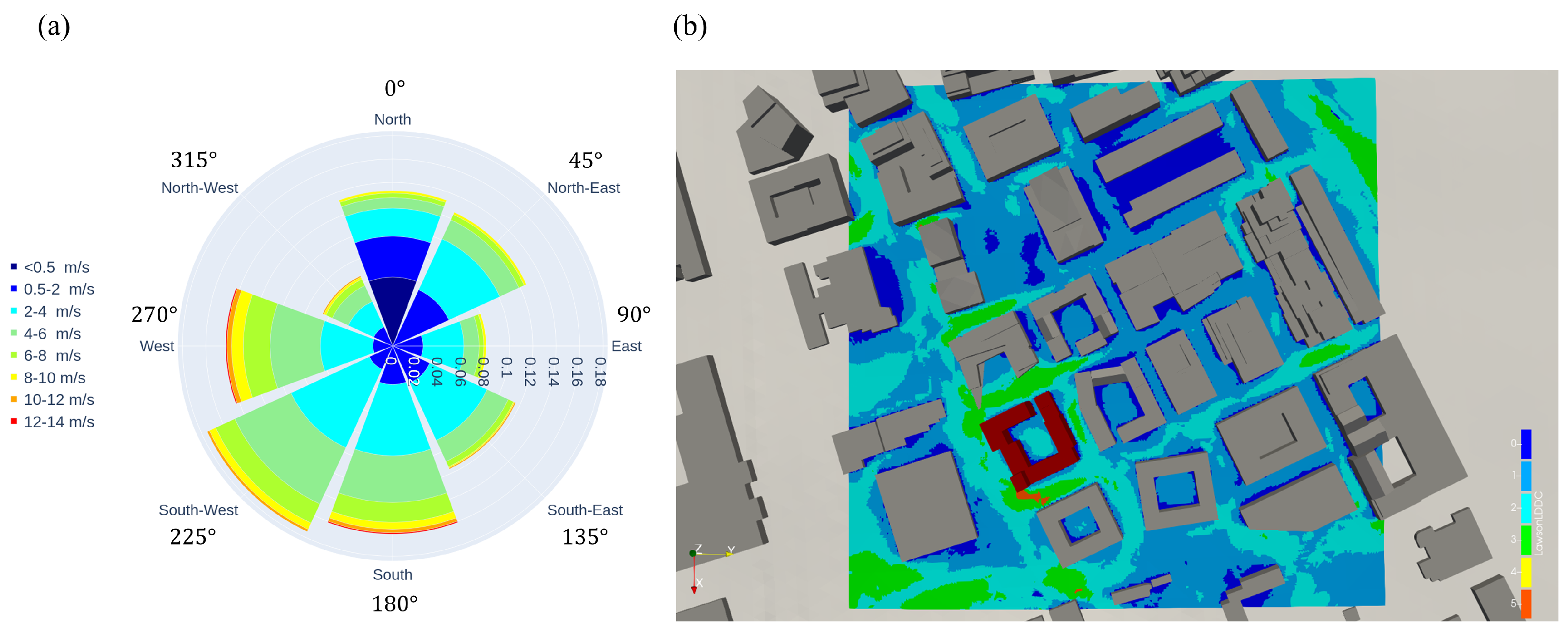
2.2. Wind Rose Statistic and Wind Comfort

Wind roses are the usual way to describe winds and wind directions graphically. All measured wind speeds and directions in a given time interval, usually on an hourly basis, are considered to derive the statistical distribution of the wind speed and direction over this time interval. It enables a comprehensive way to, e.g., determine predominant wind conditions in a given area. Wind data are commonly measured at weather stations. The wind data in this study are taken from Sweden’s Meteorological and Hydrological Institute (SMHI) at the location Göteborg A (71420) at a height of 10 m above the ground as historical data from 1961 to 2021 (see [21]). The corresponding wind rose statistic for the study area is defined as follows:
W = 0.059 0.0 0.0 0.0 0.0 0.0 0.0 0.0 0.035 0.053 0.026 0.035 0.033 0.022 0.017 0.018 0.024 0.048 0.035 0.054 0.061 0.074 0.045 0.024 0.009 0.018 0.013 0.02 0.04 0.053 0.043 0.015 0.004 0.005 0.004 0.005 0.017 0.018 0.023 0.006 0.002 0.002 0.002 0.001 0.006 0.006 0.01 0.002 0.0 0.0 0.0 0.001 0.003 0.002 0.004 0.001 0.0 0.0 0.0 0.0 0.001 0.0 0.001 0.0
where i = 1 , , 8 is the row-index of wind rose speeds and j = 1 , , 8 is the column-index of wind directions. The wind rose speeds are defined in m/s as
V = 0.5 2.0 4.0 6.0 8.0 10.0 12.0 14.0
and the wind directions are defined in ° as
A = 0.0 45.0 90.0 135.0 180.0 225.0 270.0 315.0
The corresponding wind rose can be seen in Figure 2a.
We follow the standard approach, considering the historical meteorological data and the local wind conditions obtained from simulations for wind comfort evaluation. Therefore, we run CFD simulations for 8 discrete wind directions. We use the well-established Lawson LDDC criterion (LLC) as required by the wind microclimate guidelines for the city of London [22] and described in more detail in [23]. The LLC defines wind comfort classes based on the wind speed and the statistical exceedance of the upper wind speed for each class. Exceedance is the statistical probability that a given observation will be higher than a certain threshold. The classes that we use are listed in Table 2.
This comfort criterion is conveniently applied at a pedestrian level of 1.5 m above the ground, resulting in a 2D non-planar surface. The resulting LLC for the example setting of the new building complex (see Section 2.1) can be seen in Figure 2b. The new building block, which consists of nine segments, is colored red, and all other fixed buildings are colored gray.

Extreme Case Scenarios
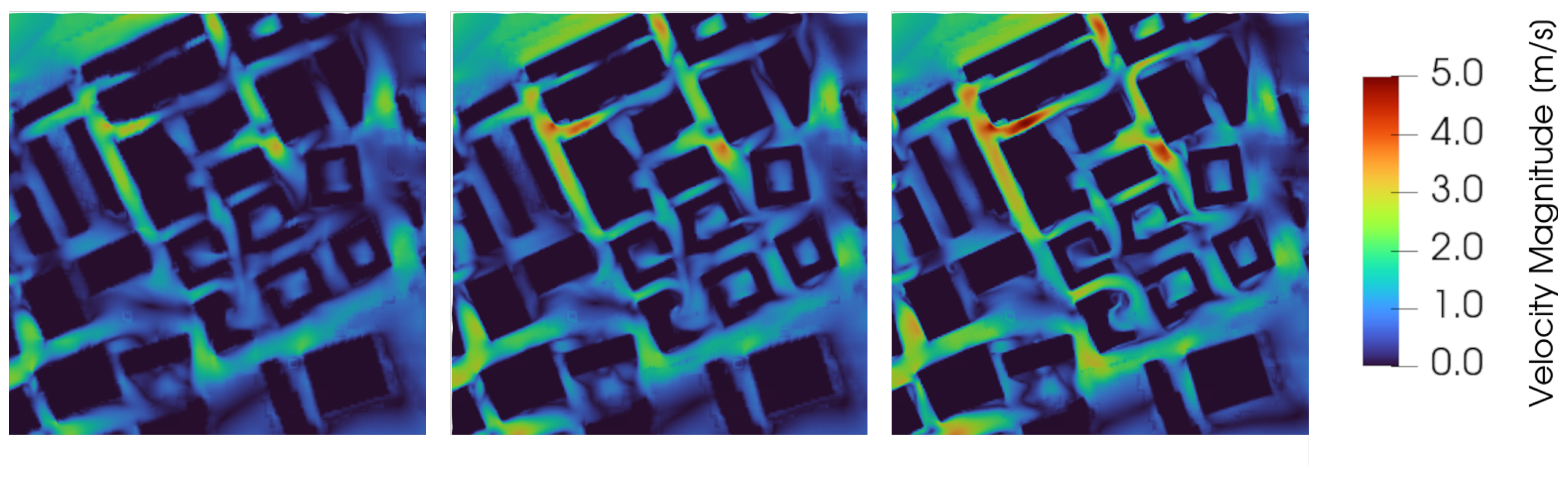
For the data augmentation strategy explained in the following, we use “extreme case LLC”. We define such an extreme case scenario, e, as follows:
e = ( V i , A j ) E = { V i , A j | i , j = 1 , , 8 } ,
where E is the set of all extreme case scenarios. The corresponding wind rose statistic for the extreme case scenario e = ( V 1 = 0.5   m / s , A 1 = 0.0 ° ) is defined, for example, as follows:
W e = 1.0 0.0 0.0 0.0 0.0 0.0 0.0 0.0 0.0 .
The wind rose statistic, W e , is 1.0 at the position of the extreme case scenario e = ( V 1 = 0.5   m / s , A 1 = 0.0 ° ) and 0.0 for all other cases. Therefore, we assume that, for an extreme case scenario, the wind blows from one direction at a specific strength with a probability of 100%. The wind speed for all other scenarios is set to 0.0 . In Figure 3, this is illustrated for an example building setup. Figure 3a shows the LLC based on the wind statistics defined in Section 2.2. Two extreme case LLCs are shown in Figure 3b,c. The scenario in Figure 3b corresponds to a wind rose speed of V 1 = 0.5   m / s and a wind direction of A 1 = 0.0 °, leading to low wind comfort. In contrast to this, the scenario in Figure 3c leads to a rather high wind comfort, because the extreme case corresponds to a wind rose speed of V 8 = 14.0   m / s and a wind direction of A 8 = 315.0 °.

2.3. CFD Simulation

Wind simulations are performed using the Immersed Boundary Flow Solver IBOFlow® [24] (IBOFlow CitySimulation 0.12.2.1), which has been validated for urban wind simulations in [25,26] and has previously been used for simulation-based optimization in [27,28,29]. The inlet profiles of velocity and turbulence properties are generated following the approach described in [30]. As the site is located in the city of Mölndal and surrounded by a mixture of homogeneous city, vegetation, and forest clumps, an aerodynamic roughness length z 0 = 0.5   m is chosen for all directions following the Davenport–Wieringa roughness classification [31]. Simulations are performed in eight discrete wind directions, with a reference inlet velocity of 5 m/s. The simulation domain consists of a circular area with a radius of ca. 700 m where the buildings are explicitly modeled, while the surrounding area without explicitly modeled buildings is of the dimension 1 km times 1 km as shown in Figure 1a,b). The mesh consists of roughly 6 million grid cells in the fluid regime and has a local resolution of 0.6 m in the vertical direction and 1.2 m in the horizontal direction. Facilitating the simulation of the different wind directions, we use a fixed Cartesian domain, and the geometries are rotated depending on the discrete wind direction. At the outlet, a total pressure boundary condition is set. On the sides and at the top of the domain, symmetry conditions are imposed. The ground and the buildings are treated as walls, using standard wall functions with sand-grain modification following [32]. We then solve the steady-state Reynolds-averaged Navier–Stokes equations, including the k-g SST model [33], a variant of the well-known k- ω SST model [34,35]. A grid study is performed, and the results of the velocity distribution for three different meshes are shown in Figure 4. The three meshes contain 2.7 million cells with a local resolution of 1.2 m in the vertical direction, 6 million cells with a local resolution of 0.6 m in the vertical direction, and 21 million cells with a local resolution of 0.3 m in the vertical direction, respectively. The corresponding simulation times for a single directional run are 1.75 h, 3.25 h, and 31 h, respectively. The large difference in computational time between the middle and the finest mesh stems from both the larger number of cells and the increase in required iterations until convergence is reached. It can be seen that grid convergence is not yet established with the middle mesh. However, for the sake of restricting computational time in this feasibility study, we chose the mesh containing 6 million cells, as the important flow properties are captured properly. Running a complete simulation including all eight wind directions (see Section 2.2) therefore takes about 26 h.

2.4. Performed Simulations

To create the training data for the CNNs, we performed 200 simulations with the CFD solver. Simulations were run on a cluster of dual Intel Xeon Gold 6240R CPU cores in parallel in groups of 30 to 40 simulations each.
We set the heights of the individual nine segments of the new building (see Table 1) of these 200 simulations randomly using Sobol sequences [36], to make sure that the training space was distributed evenly. For these 200 simulations, the height of each segment of the new building is different and is allowed to be in the range of 3 to 15 floors, corresponding to a range of 10 to 46 m. The first floor has a height of 4 m and the floors above the first floor each have a height of 3 m. In addition to the 200 simulations, we performed 13 simulations, where the height of the nine segments is the same, ranging from 3 floors to 15 floors. These simulations are incorporated into each training data set (see Section 4) to ensure that the network captures these extreme cases where segments have the same height.
We performed another 25 simulations not included in the training set for testing purposes.

3. Machine Learning Models

In this Section, the ML model is described. We analyze two different models in this work: a regression model and a classification model. For both models, we use a CNN architecture described in the following.

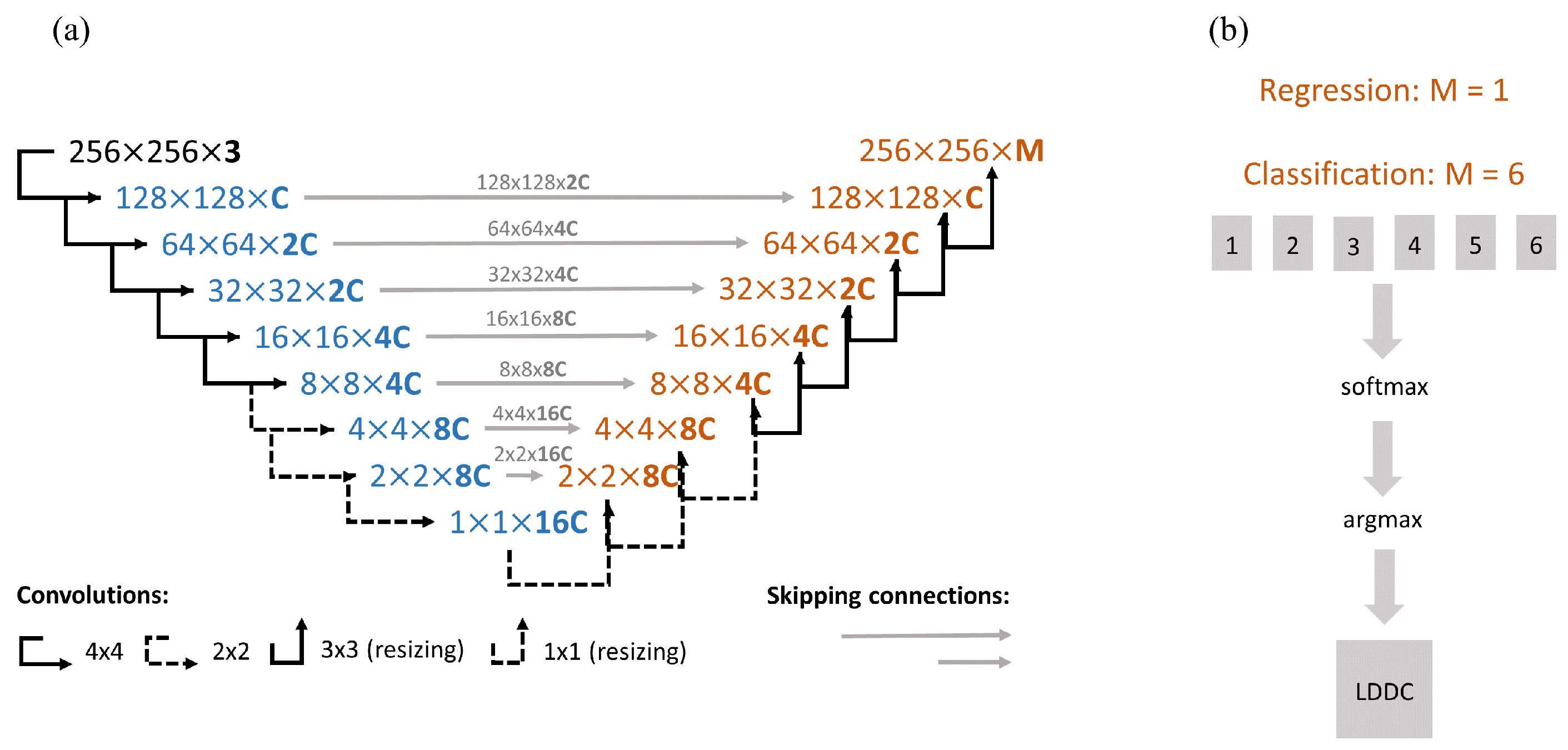
3.1. Architecture of the CNN

We use a convolutional neural network (CNN) to predict wind velocity and LLC. The U-Net was first introduced to the ML community in 2015 by [11]. It was originally developed for biomedical image segmentation tasks but has also become popular in other research areas such as audio source separation, road extraction, and speech enhancement/speech de-noising (see [37,38,39]). In this work, adapt the U-Net architecture from [13], where the U-Net predicts the wind velocities and pressure around two-dimensional airfoil sections, and therewith follow-up on the work in [29]. The U-Net can generalize based on relatively few training data (see [11]). This property is advantageous for training an ML model based on time-consuming CFD simulations.
The architecture of the U-Net is visualized in Figure 5a. It consists of a contracting path (encoder) and an expanding path (decoder).
The encoder (left side, highlighted in blue) consists of the repeated application of encoding blocks downsampling the input. More specifically, this is achieved by applying 4 × 4 and 2 × 2 convolutions in combination with a stride of 2, and a padding of 1 for the 4 × 4 convolution and a padding of 0 for the 2 × 2 convolution, respectively. The number of inputs defines the number of starting channels, which in our case is 3. The number of channels is doubled repeatedly on the way down so that at the deepest layer there is a 1 × 1 data point across the number of channels. The number of channels, C, is given by
C = 2 L ,
where L is the channel exponent.
The decoder (right side, highlighted in orange) consists of the repeated application of decoding blocks upsampling the data point to the desired output resolution. This is done by applying 3 × 3 and 1 × 1 convolutions in combination with a stride of 1, and a padding of 1 for the 3 × 3 convolution and a padding of 0 for the 1 × 1 convolution. The number of channels decreases on the way up so that the desired number of outputs, M, is reached on the output layer (typically the number of channels is divided by two).
Each encoding and decoding block consists of a convolutional layer, a batch normalization layer, and a non-linear activation function. As proposed in [13], we use leaky- ReLU activation functions with α = 0.2 for the encoding blocks and ReLU activation functions for the decoding blocks. In this case, the encoder consists of four 4 × 4 and three 2 × 2 convolutions, and the deepest layer is a 1 × 1 data point over 256 channels. The decoder consists of three 1 × 1 convolutions and four 3 × 3 convolutions for resizing.
The regression model has one output ( M = 1 ) and is trained on velocity. We use L 1 loss for training.
We train the classification model on the LLC consisting of 6 classes, and thus the number of outputs M = 6 , one for each class. This results in a 6 × 256 × 256 tensor. Then, we apply the softmax function implemented in the Python package PyTorch [40], which is defined as
softmax ( x i ) = exp x i j exp x j .
The softmax function is commonly used in machine learning and deep learning for multi-class classification tasks [41]. It rescales the elements of the 6 × 256 × 256 tensor, such that the output probabilities are non-negative and sum up to 1. This property is important for interpreting the output as probabilities. After this, we apply the argmax function implemented in PyTorch [40], which is used to find the class with the highest probability of becoming the predicted class in the input tensor across one dimension. This yields one output, i.e., a 1 × 256 × 256 tensor containing LLC classes. For the classification model, we use the cross-entropy loss for training. This process is visualized in Figure 5b.

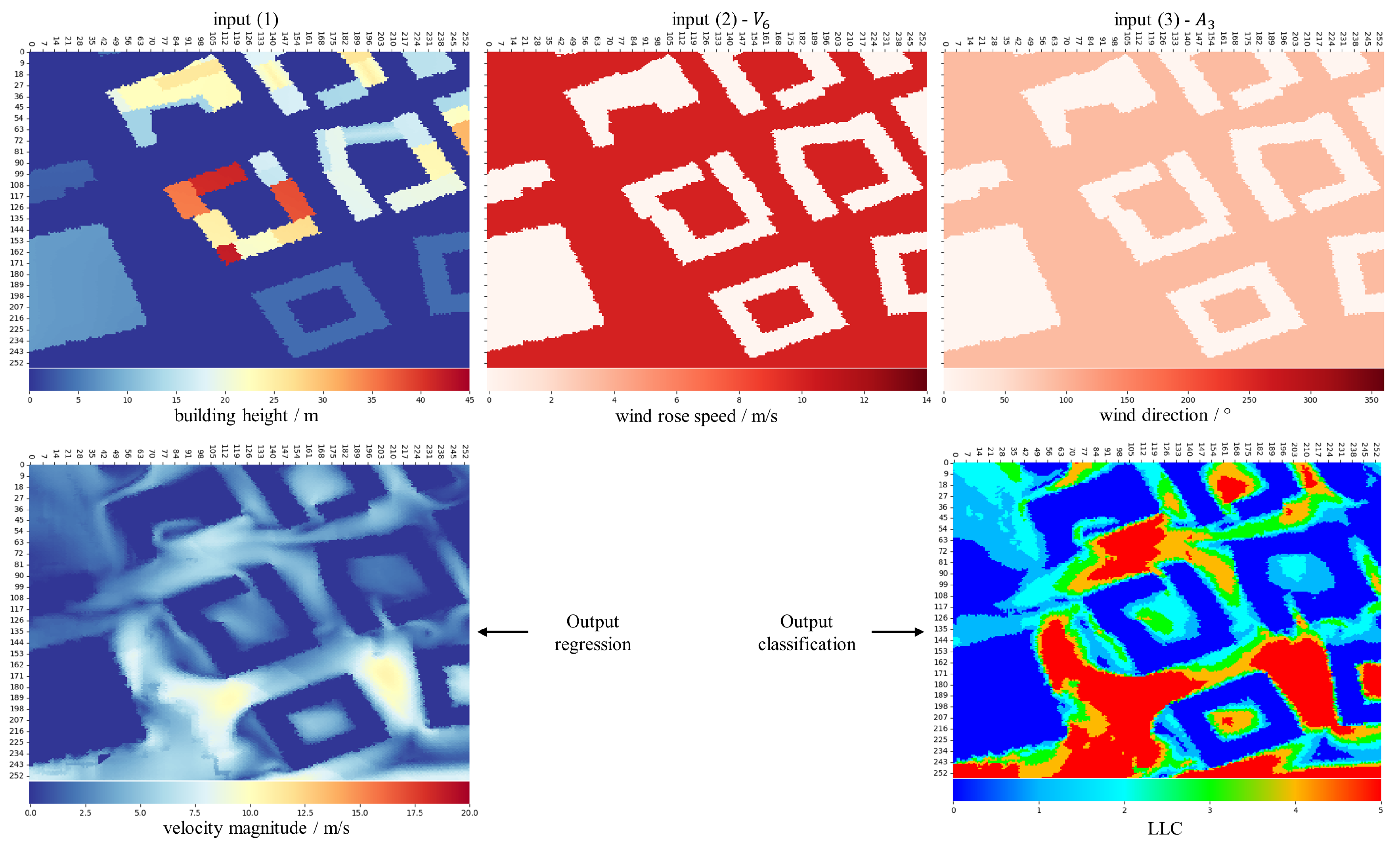
3.2. Inputs and Outputs

The following aspects are described using a specific building setup.
The CNN input for both the classifier and the regression model consists of three matrices representing the town mask with building height information (1) in m, the wind rose speed (2) in m/s, and the wind direction (3) in °. Each matrix consists of a set of pixels P. In our case, all matrices are resolved with 256 × 256 pixels, p P .
The indices of input (1) contain zero if there is no building. Otherwise, they are set to the corresponding building height. The indices of inputs (2) and (3) are set to zero if there is a building at that position. Otherwise, they are set to the wind rose speed and wind direction, respectively. Therefore, inputs (2) and (3) correspond to an extreme case scenario e = ( V i , A j ) . For an extreme case LLC, e, we assume the entry of the wind rose statistic corresponding to the wind rose speed and wind direction to be 1.0 , while all the other entries are 0.0 (see Section 2.2).
The CNN output for the regression model consists of one matrix with the corresponding speed, i.e., magnitude of the velocity vector in m/s for e. The CNN output for the classification model consists of one matrix containing the extreme case LLC for e. Each pixel of the matrix contains a class label in the range of 0 to 5 for the six LLC classes. An example of an unnormalized training sample for the CNN is shown in Figure 6. The output for the regression model is shown on the left side in the lower row, and the output for the classification model is shown on the right side in the lower row of the picture.
We use normalized training samples for CNN training. Input (1) is normalized with respect to the tallest building in the area, while inputs (2) and (3) are normalized with respect to the highest wind rose speed and the highest wind direction, respectively. The output is normalized to the [ 0 , 1 ] range. We use the maximum absolute value for the velocity computed over the entire training data set to normalize the data. The classification model output is class labels, where normalization is unnecessary.

3.3. Decision Tree Classifier
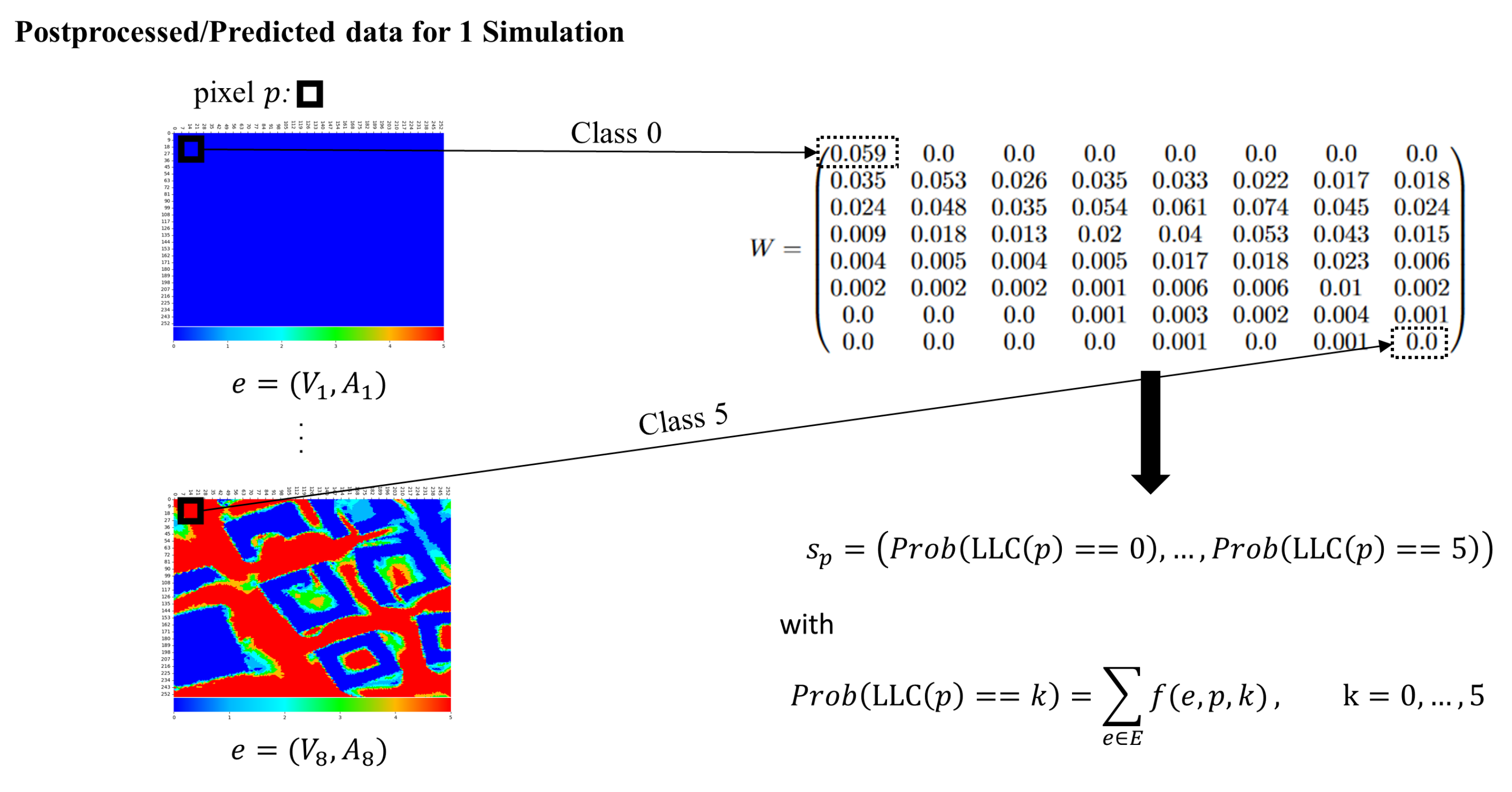
Since the classification model predicts the extreme case LLC, a “data accumulator” is necessary to predict the LLC for the wind rose statistic, W. Data accumulation (DA) is performed utilizing a simple additional classification model.
Decision tree classification (DTC) uses a decision tree to predict discrete values. A decision tree is constructed by recursively generating decision rules and splitting the training data set into smaller subsets according to that rule (see [42]).
In this work, we are using the DTC implementations of the Sklearn library [43].

Data Accumulation

For each pixel, p P , we calculate the probability that the LLC for wind rose statistic W for this pixel equals class k, defined as follows:
P r o b ( LLC ( p ) = = k ) = e E f ( e , p , k ) ,
where f : E × P × K [ 0 , 1 ] , with P the set of all pixels, and K : = { 0 , , 5 } the set of class labels, defined as follows:
f ( ( V i , A j ) , p , k ) = W i j , if LLC ( e , p ) = k 0 , otherwise
for each scenario, e = ( V i , A j ) , i , j = 1 , , 8 , where W is the wind rose statistic defined in Equation (2). This results in the vector, s p , of probabilities for the class labels, K, for each pixel, p, defined as follows:
s p = P r o b ( LLC ( p ) = = 0 ) P r o b ( LLC ( p ) = = 5 )
This process is visualized in Figure 7 for one pixel, p. Repeating this process for every pixel, p P , leads to set S:
S = { s p | p P }
Regarding numerous simulations, the DTC is trained on multiple sets of S and for each pixel, p P , it predicts the LLC label, k, for the wind rose statistic, W:
DTC : s p k .

3.4. Post-Processing and Augmenting CFD Simulations for Training

For a simulation setting, i.e., a specific setup of the new building, the CFD solver performs an individual simulation with 8 different sub-simulations, 1 for each wind direction. For each of those sub-simulations, the inlet velocity is constructed as described in Section 2.3, with a reference velocity of u = ( u x , u y , u z ) = ( 5   m / s , 0   m / s , 0   m / s ) at reference height 10 m. For each sub-simulation, the geometry is rotated around the z-axis by the wind direction. When all sub-simulations are finished, the LLC is calculated using the wind rose statistic (see Section 2.2).
To post-process the training data for CNN from the CFD simulations, we can take advantage of the fact that the fluid data are available for each of the eight wind directions per simulation, i.e., we have access to the velocity fields for each wind direction, A j . Furthermore, we take advantage of the fact that the velocity fields are in the Reynolds-similar regime and thus can be linearly scaled with the reference inlet velocity, see e.g., [26]. In this way, we can generate even more training data for each wind rose speed, V i . In principle, this means that we can post-process one training sample for each entry of the wind statistic (2), i.e., for each extreme case scenario, e (see Section 2.2).
There is a slight difference between post-processing for the regression and classification models. On the one hand, the regression model is trained on the velocity magnitude for each extreme case scenario, e. The goal is to predict the magnitude of the velocity for the reference velocity of 5 m/s for each wind direction. From this, we can calculate the LLC. We, therefore, include the reference velocity of 5 m/s in the training data, resulting in the wind rose speed vector for training in m/s:
V ˜ = 0.5 2.0 4.0 5.0 6.0 8.0 10.0 12.0 14.0 .
Thus, we can post-process 72 training samples from each simulation—64 training samples from the wind statistic and another 8 training samples for each wind direction with respect to the reference velocity.
The classification model is trained on the extreme case LLC, on the other hand. From this, we predict the LLC for the wind rose statistic, W, for a specific setting of the new building (see Section 3.5). In this case, we do not include the reference velocity, and thus we can post-process 64 training samples from each simulation. We obtain the velocity magnitude information for the corresponding extreme case scenario, e, from the simulation, and from this we calculate the extreme case LLC.

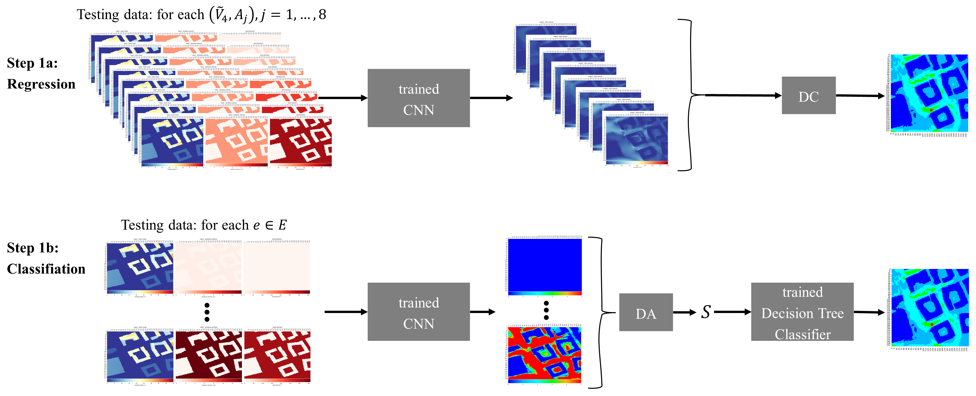
3.5. Machine Learning Workflow

The first step of the MLW is training the regression and classification models. During the training step, the CNN is trained with the training data consisting of three inputs and one output, as described in Section 3.2. This step is the same for the regression and the classification models, except that the architecture of the U-Net is different, and we use different losses for regression and classification (see Section 3.1). Furthermore, depending on whether the regression or the classification model is trained, different training data are used, as described in Section 3.4.
The MLW for the prediction step is visualized in Figure 8 and is described in more detail for regression and classification in the following.

3.5.1. Prediction Workflow for Regression Model

The trained CNN predicts the velocity for a given input sample. To predict the LLC, we feed the CNN eight input samples, where inputs (1) (town mask) and (2) (wind rose speed) are fixed to a specific setting of the new building and the reference wind rose speed V ˜ 5 = 5   m / s , respectively. Input 3 includes the eight different wind directions, A j . We obtain a velocity prediction from the trained CNN for each input sample. Before calculating the LLC, we perform a data completion (DC) step, where the prediction for each wind direction, A j , is scaled to each wind rose speed, V i , resulting in 64 matrices. From this, we can then calculate the LLC. This process is illustrated in step 1a of Figure 8.

3.5.2. Prediction Workflow for Classification Model

In the case of the classification model, the trained CNN predicts the extreme case LLC for a given input sample. The MLW for classification is illustrated in step 1b of Figure 8.
To predict the LLC, we feed the CNN 64 input samples, one input for each extreme case scenario, e. Input (1) (town mask) is fixed to a specific setting of the new building. Inputs (2) and (3) (wind rose speed, V i , and wind direction, A j ) include the 64 extreme case scenarios, e (see Section 2.2). In the first step, we obtain an extreme case LLC prediction for this specific scenario of the new building for each of these 64 test samples. In a second step, the data accumulation (DA) step is performed, which is described in Section 3.3, resulting in set S containing all vectors, s p , of probabilities for the class labels, K, for each pixel, p, of the LLC for the wind rose statistic, W. The LLC is determined pixel-wise in a third step by feeding the DTC each probability, s p . The DTC in turn predicts the class label, k, for each pixel of the LLC for the wind rose statistic, W.

3.6. Error Metrics

The following standard metrics are considered to measure the performance of the trained CNN. Absolute error (AE) measures the absolute difference between the predicted and actual values. It gives the magnitude of the error without considering the direction. AE is useful in evaluating the overall accuracy of a prediction model. Mean absolute error (MAE) provides a measure of the average magnitude of the errors. MAE is commonly used to compare the performance of different models or algorithms, as it indicates how close the predictions are to the actual values on average. Relative absolute error (RAE) is a normalized version of MAE that takes into account the scale of the data. RAE is useful when comparing models on data sets with different scales, as it allows for a fairer comparison by considering the baseline performance.
For the target with the corresponding prediction, the absolute error for a specific pixel, p, in the output matrix is defined as
AE p = target p pred p .
For any given test sample, the mean absolute error between the prediction and the target is defined as
MAE = 1 | P | p P target p pred p .
The absolute target average of the target is defined as
ATA = 1 | P | p P target i , j .
The relative average error of the prediction compared with the target is
RAE = MAE ATA .
To measure the performance for the entire test set, the mean of RAE is calculated as,
RAE ¯ = 1 N n = 1 N RAE ,
where N is the number of test samples.
Furthermore, we consider the F 1 -score metric (see [44]) to measure the accuracy of the predicted LLC. The F 1 -score for a class k is defined as follows
F 1 ( class = k ) = 2 precision ( class = k ) · recall ( class = k ) precision ( class = k ) + recall ( class = k ) ,
with precision for class k defined as
precision ( class = k ) = TP ( class = k ) TP ( class = k ) + FP ( class = k ) .
Recall for class k is defined as
recall ( class = k ) = TP ( class = k ) TP ( class = k ) + FN ( class = k ) .
TP, FP, and FN correspond to “true positive”, “false positive”, and “false negative”. More specifically, TP ( class = k ) indicates how many pixels, p, with the true label k are predicted correctly by the model, i.e., the model also predicts class k. FP ( class = k ) gives the amount of pixels, p, that are predicted with label k, but belong to a different class, and FN ( class = k ) indicates the amount of pixels, p, that are incorrectly predicted with a class different from k.
In our case, the LLC consists of six classes. The F 1 -score is calculated for each class individually, resulting in six scalar values. To receive a single scalar value, we use the averaging method macro, taking the average of the F 1 -score of each class. The macro-averaging method gives equal weight to each class, independent of the number of instances. Thus, the overall F 1 -score is defined as follows:
F 1 = k K F 1 ( class = k ) | K |
We use the F 1 metric to measure the performance of the classification model, and we also consider this metric for evaluating the performance of both models (regression and classification) on the LLC test set. Furthermore, we consider the recall metric for each class. This is appropriate here because the LLC consists of classes.

4. Training Results

Three different training data sets were used for training the CNNs. Each of these training data sets included 13 simulations with an equal number of floors for each segment (ranging from 3 to 15 floors). Then we randomly added 50 and 100 simulations from the 200 performed simulations (see Section 2.4), resulting in the first two training data sets. Thus, the third training data set included 200 simulations plus 13 simulations. The resulting number of training samples for the regression and classification models after applying the augmentation strategy described in Section 3.4 are listed in following tables.
Before training the models on each data set, we performed hyperparameter optimization using Optuna (see [45]). The corresponding hyperparameters are listed in Table 3. After training, we tested the networks with respect to 25 separate simulations.

4.1. Regression Model

4.1.1. Hyperparameter Optimization
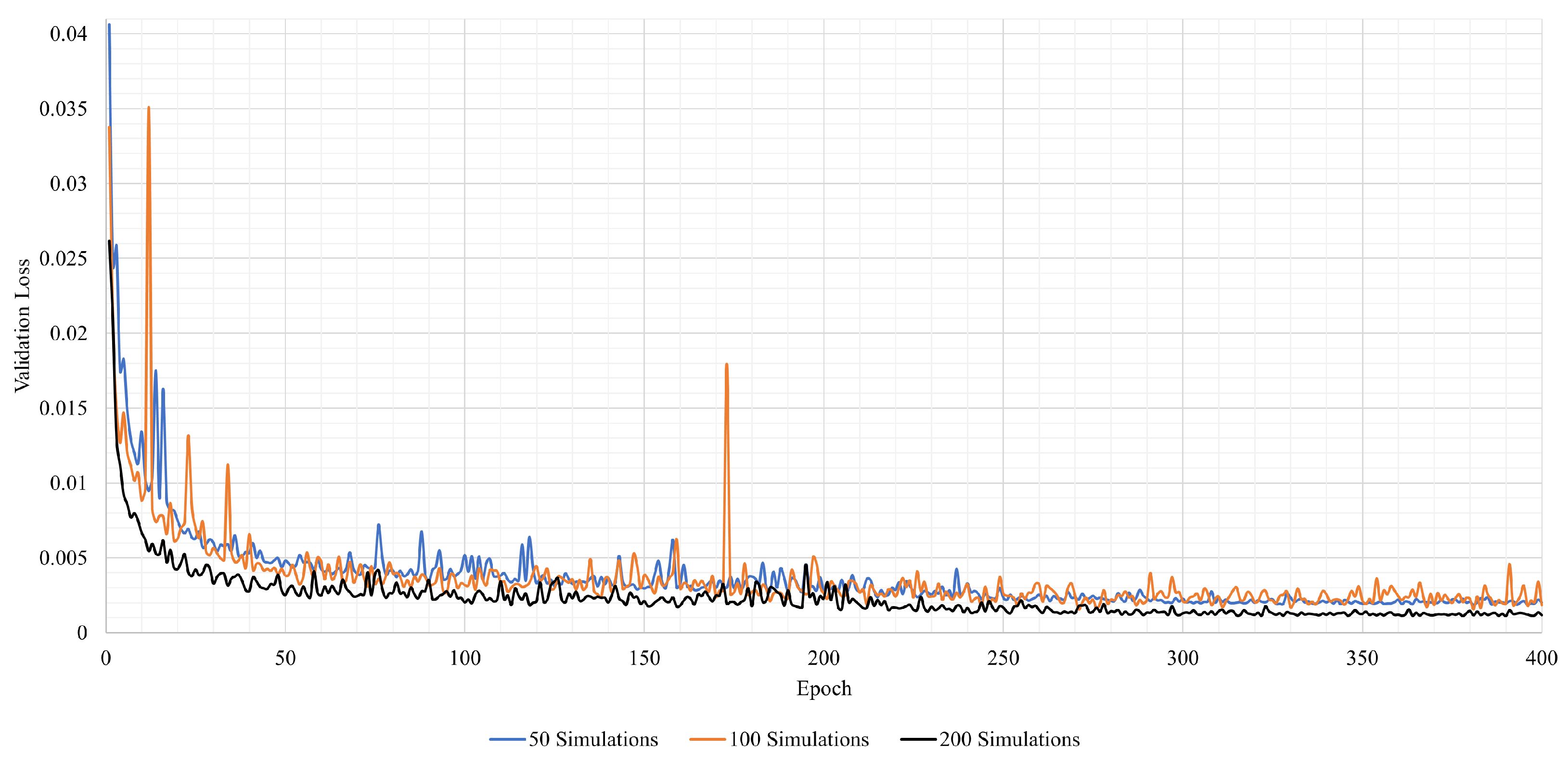
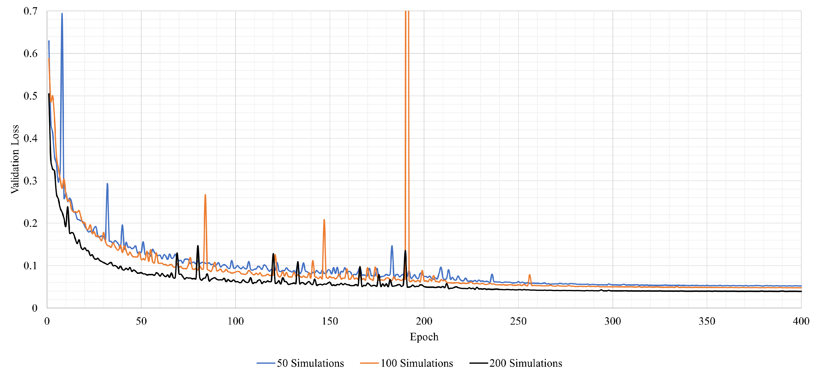
The best-performing hyperparameters are displayed in Table 4. In almost all our models, we observe the highest number of channels because the problem at hand is complex. A higher number of channels was not possible for memory reasons. This may indicate an overfitting effect. However, as the validation loss curves in Figure 9 decrease over time, they reach a plateau, suggesting that there is no overfitting. The optimal batch size of 6 is small compared with typical batch sizes. The reason for this is that we are working with smaller data sizes and that the network is deep and complex. However, this also affects the training of the model, so the model can skip the local minima of the loss function more easily. The optimal dropout probability is close to zero, specifically for a larger number of simulations. That indicates sufficiently diverse data. Also, since we make use of a decaying learning rate, that is enough regularization for the model. The optimal learning rate is neither too low nor too high, leading to the fastest convergence.

4.1.2. Training

We trained three individual regression models based on the different training sets and optimal parameters in Table 5. The number of training samples was obtained by the augmentation strategy for the regression, described in Section 3.4. For each one of the 64 entries of the wind rose statistic and for each simulation, we generated one training sample. Also, for each one of the eight wind directions, the reference wind rose speed, and for each simulation, we generated one training sample. Thus, for example, for 50 + 13 simulations, this results in 63 × ( 64 + 8 ) = 4536 training samples.
The models were trained for 400 epochs. Figure 9 shows the validation loss curve for each model. Training the regression model based on 50 and 100 simulations leads to a comparably higher validation loss after 400 epochs than training based on 200 simulations. Furthermore, the oscillations in the validation loss are the smallest for the model “200 Simulations”.

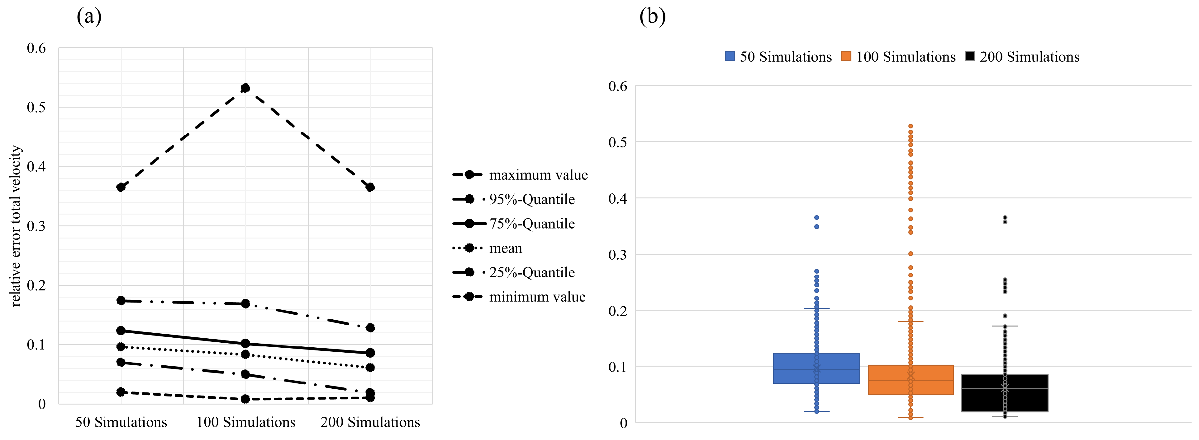
4.1.3. Performance on Test Set

The performance on the test set for each of the models is shown in Figure 10. As expected, the more data that were used for training, the better the performance on the test set was. Figure 10 shows different quantiles of the test set. Analyzing, for example, the mean, one notices that the mean is highest for the “50 Simulations” model. This is true for all the other quantiles, except for the maximum value, which is highest for the “100 Simulations” model. The “200 Simulations” model performs best on the test set. The mean of the RAE ¯ of the velocity equals 0.0610 . This corresponds to a value of 1.22 m/s. Also, 95% of the test samples result in a RAE ¯ of less than 0.1281 , which equals about 2.56 m/s.
The distribution of the test set for each model is shown in the form of a box plot in Figure 10b. The box represents the data lying within the 25% and the 75% quantile. The horizontal line within the box corresponds to the median of the data. There are a few outliers present, which are marked by the dots above the upper whiskers. Here, it is also clear that the “200 Simulations” model performs best on the test set. The median is the smallest for this box plot (see Figure 10). Furthermore, there are fewer outliers present than there are for the other two models. Compared with the other models, most outliers can be seen in the “100 Simulations” model. The reason for that could lie in the comparably higher validation loss of the “100 Simulations” model (see Figure 9).

4.1.4. Discussion

In summary, the “200 Simulation” model performs the best on the test set, with a mean relative absolute error ( RAE ¯ ) of 0.0610 . However, when compared with the best-performing models in [13,14], these errors are higher. For example, [13] achieved a relative error of approximately 0.03 . One main difference is that [13] had access to many more data, with up to 25,600 individual simulations for training. They also trained a network with only 200 individual simulations, which resulted in an error similar to ours of about 0.06 . However, they did not perform any data augmentation. Another significant difference is that [13] investigated a different use case—an airfoil with no surrounding geometries. In our case, we are dealing with a building consisting of multiple segments surrounded by other buildings. This leads to more complicated wind profiles, which could explain the higher errors and outliers in the data. This observation is also consistent with the findings of [14], who observed that including more buildings in the training samples resulted in higher errors due to more complicated wind profiles.

4.2. Classification Model

4.2.1. Hyperparameter Optimization

For the classification model, optimal hyperparameters are displayed in Table 5. The overall behavior is very similar to the regression models in Section 4.1.1. Also, here the number of channels is at the maximum. An additional increase in the number would improve the model even further. However, that requires additional memory allocation. One difference is the increase in the batch size. However, it is not that significant and considerably small, thus leading to the same interpretation.

4.2.2. Training

We trained three classification models based on the three training data sets and optimal parameters in Table 5.
Each model was again trained for 400 epochs. Figure 11 shows the corresponding validation loss curves for each model. Here, training the “200 Simulations” model leads to a comparably smaller loss after 400 epochs of 0.03917 , than training the other two models.

4.2.3. Decision Tree Classifier Training

The training data for the DTC were obtained from the training sets, as described in Section 3.3. A total of 25% of these data were set aside for testing. The training data set is imbalanced because there are significantly fewer samples of class 5 present than there are of the other classes (see [46]). For this reason, we performed oversampling before training the DTC on each training data set (50, 100, and 200 simulations). We used the Synthetic Minority Oversampling Technique (SMOTE) implemented in the Python package imblearn (see [47]) to balance our data sets. The SMOTE algorithm adds new artificial samples to the data set by first selecting a minority class instance. It finds its k nearest minority class neighbors and randomly selects one of those. A new point is then added by interpolating between the selected point and the selected neighboring point (see [46]).
Before training, we also performed hyperparameter optimization to tune the hyperparameters. Tuned hyperparameters for the DTC are the maximum depth of the tree and the minimum number of samples a leaf must have. The parameter ranges are given in Table 6. The hyperparameter optimization was performed by using grid search with 5-fold cross-validation (implementation of the Sklearn library [43]). The resulting hyperparameters are also given in Table 6.
The performance on the test set of the DTC classifier for each training set is given in Table 7. For all three training sets, the accuracy on the corresponding test set is greater than 96%.

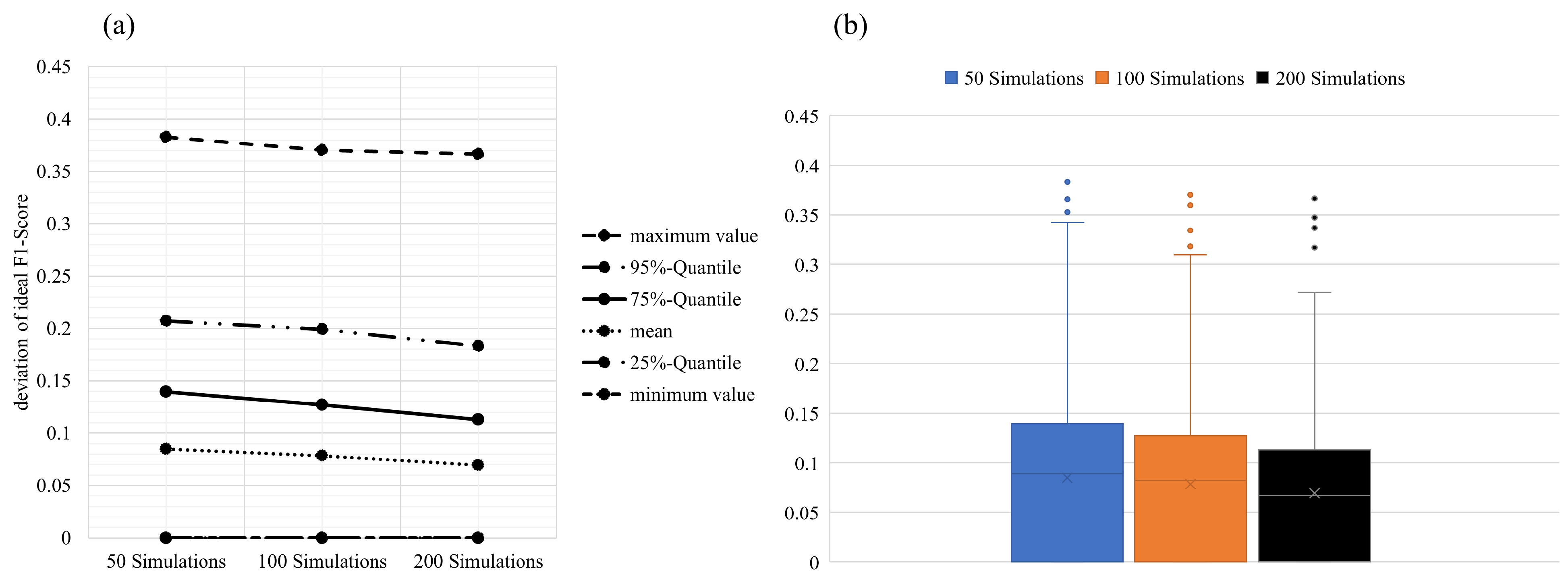
4.2.4. Performance on Test Set

The performance on the test set for each model is shown in Figure 12. We consider the deviation of each sample from the ideal F 1 -score of 1 as a metric. In Figure 12a, different quantiles of the test set are plotted. For example, analyzing the 95% quantile, one notices that the deviation of 95% of the data from the ideal F 1 -score for the “200 Simulations” model equals 0.1832 . In other words, 95% of the data yield an F 1 -score of at least 81.68 %.
Due to the augmentation strategy we used for the classification model (see Section 3.4 and Section 3.5), there are a few samples where the entire output matrix equals class 0. These samples are always predicted correctly and yield an F 1 -score of 1. The higher the wind rose speed is, the more classes there are that appear in the output matrix (the extreme case LLC). Those samples yield lower F 1 -scores. An example is shown in Figure 13. This test sample is predicted with model “200 Simulations” and yields an F 1 -score of 91.27 %. The figure shows the prediction on the left side and the expectation on the right side. The extreme case LLC is predicted well for this test sample, except for a few details.
Overall, the three classification models yield a mean of the deviation from the ideal F 1 -score of 0.0849 , 0.0784 , and 0.0692 , for the “50 Simulations”, “100 Simulations”, and the “200 Simulations”models. This corresponds to an average F 1 -score of 91.51 %, 92.16 %, and 92.08 %, respectively. The distribution of the deviation from the ideal F 1 -score is shown in the form of box plots in Figure 12b.

4.2.5. Discussion

The best-performing model on the test set is once again the “200 Simulations” model, achieving an average F 1 -score of 92.08 % . This outperforms the results of [18], who achieved a maximum F 1 -score of 89 % . There are several key differences between our approach and theirs. Firstly, while they predict three wind comfort classes, our model is capable of predicting six classes. Additionally, the use case in their study differs from ours. They consider multiple geometries without surrounding buildings, whereas our classification model predicts the extreme case LLC for entire areas, resulting in a matrix instead of a single value.

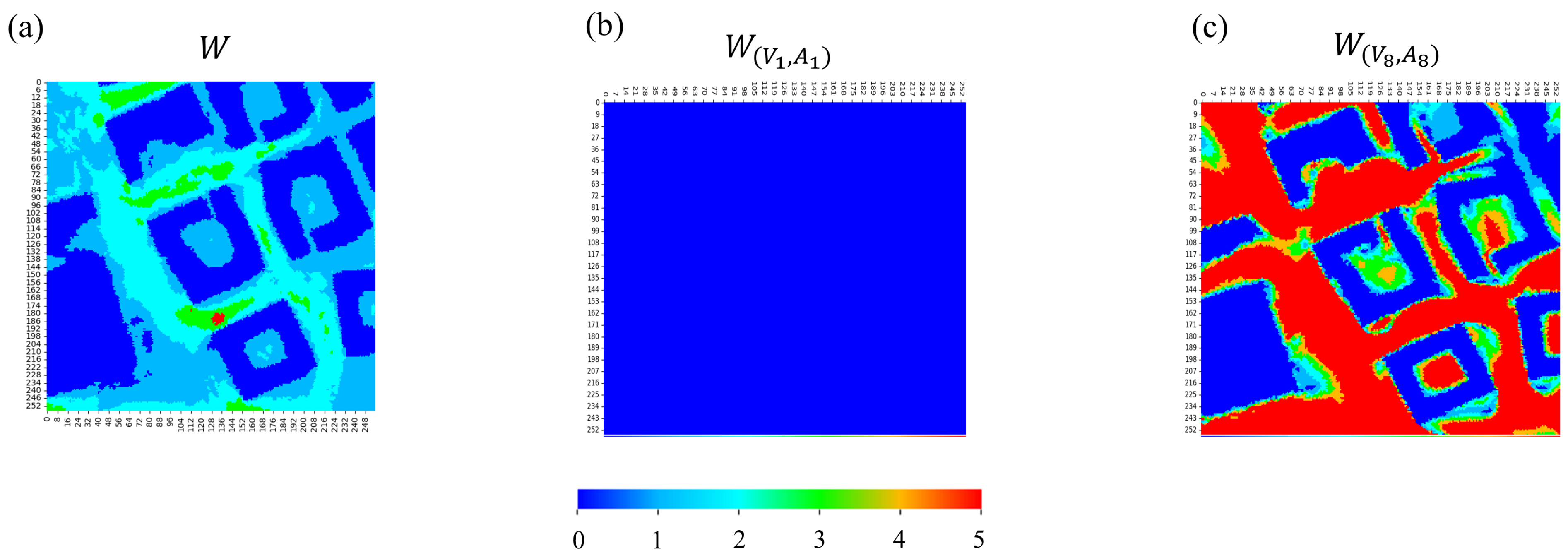
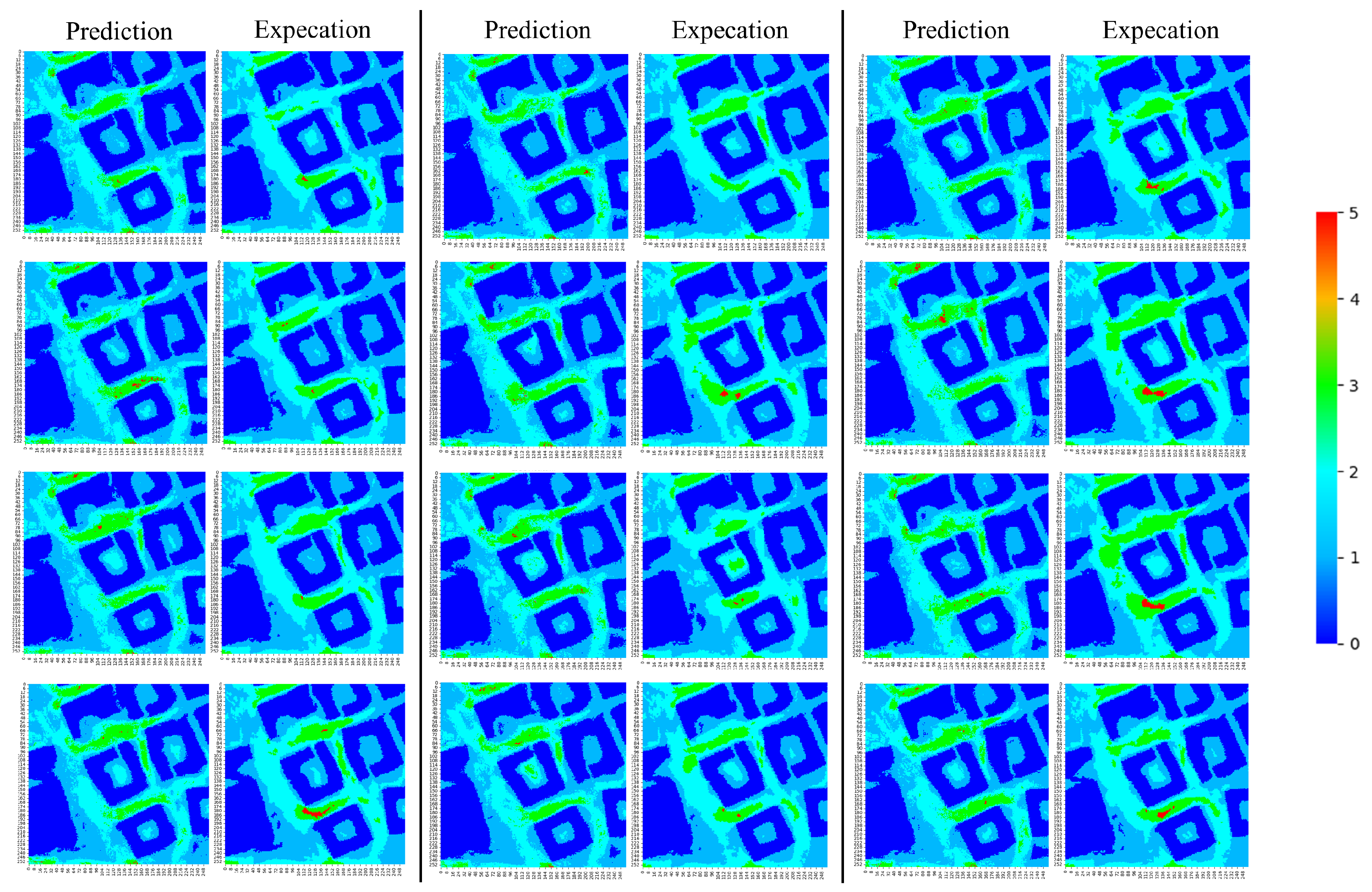
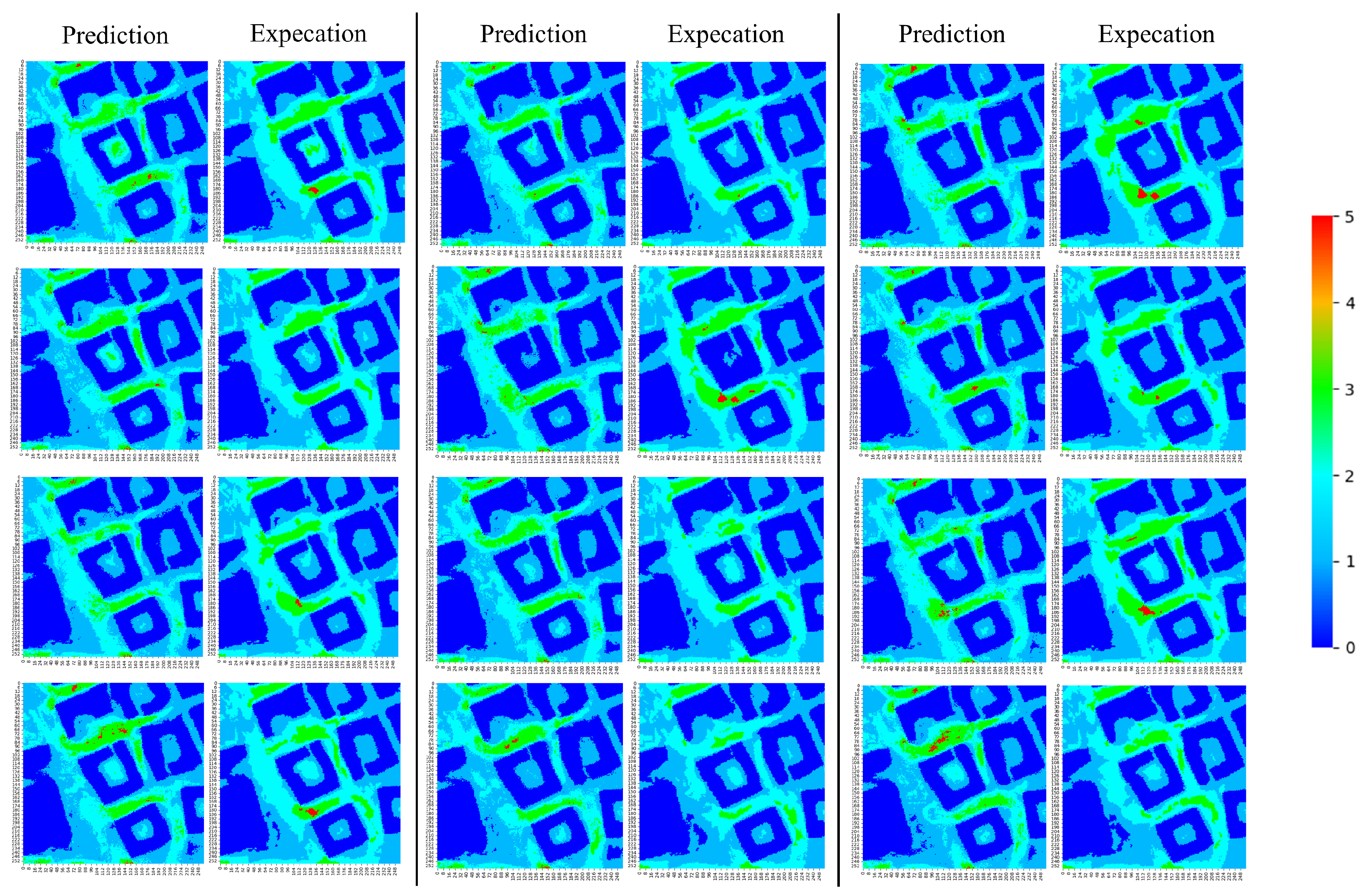
4.3. Wind Comfort Predictions with Regression and Classification Models

In both MLWs (see Section 3.5), we calculate the LLC as a post-processing step resulting from the model predictions. For the regression model, the LLC is calculated based on the prediction of the reference wind rose speed magnitude of 5 m/s for each wind direction of the wind rose statistic. The better the velocity prediction is, the better the LLC prediction can be expected to be. It is important that the model reflects the overall velocity behavior well and that the maximum velocities occurring in each scenario are predicted as accurately as possible, as these contribute to the highest class in the LLC criterion, which is concerned with pedestrian safety. Therefore, we analyze the models with respect to the overall LLC as well as with high attention to the performance of the highest LLC class.
The LLC based on the classification model is predicted using a decision tree classifier (DTC) trained on the same post-processed simulation data as the classification model itself (see Section 3.5). Here, it is important to have a well-performing classification model to predict the LLC based on the extreme case LLC.

4.3.1. Regression Model

The performance of the regression model on the LLC test set is summarized in Table 8 under “Regression”. The average F 1 -score per sample is >80% for all three models. It is best for the “200 Simulations” model, with an F 1 -score of 84.48 %. However, it is important not only to represent the overall behavior of the wind well in the LLC, but also the highest class 5 especially. Therefore, the average of the recall metric on the test set is given separately for each class in Table 8. Note that class 4 is not listed in Table 8. This is due to the fact that, in the calculation of the LLC, class 4 is very unlikely and thus rarely occurs. For the test set, class 4 indeed never occurs.
Class 0 (“Recall class 0” in Table 8) yields a high recall of over 95% for each model. This is not surprising, because class 0 mostly occurs at pixels, where buildings are present, meaning the total velocity is 0 m · s 1 . Class 1 is also predicted with high certainty and yields a recall of up to 81.73 %. Classes 2 and 3 are predicted correctly slightly less often. Here, the model “200 Simulations” performs best, with a recall of 79.50 % for class 2 and with a recall of 68.24 % for class 3. The recall for class 5 (”Recall class 5” in Table 8) is best for the model “50 Simulations”, with a value of 26.59 %.
Comparing the average recall for class 5 to this metric for the other classes in Table 8, one notices that these values are significantly smaller. We observe in the test set that the regression model often underestimates and sometimes overestimates the velocity magnitude. Therefore, class 5 of the LLC is underestimated or overestimated as well. Since the threshold for class 5 is only 0.022 % (see Section 2.2), a slight over- or underestimation of the velocity magnitude results in poor predictions for class 5.
For further analysis, we consider the “200 Simulations” model to be the best model, because the performance for all classes (except classes 1 and 5) is better than for the other classes and it yields the highest F 1 -score.
Test sample 4 is shown in Figure 14. The prediction of the LLC is shown on the left side, and, on the right side, the expected LLC from the CFD solver is shown. This sample scores an F 1 -score of 83.84 % and a recall of 31.31 % for class 5. Classes 0, 1, and 2 yield a recall of 98.63 %, 79.08 %, and 72.26 %. The recall of class 3 equals 61.89 %. The overall LLC is predicted well. Here, the behaviour of overestimating the velocity magnitude can be seen, for example, in the upper region of the prediction, where the red area is much larger than expected. Furthermore, the green area in the left region of the prediction is smaller than expected. The comparison of prediction and expectation for the other samples of the test set are shown in Appendix A, in Figure A1 and Figure A2.

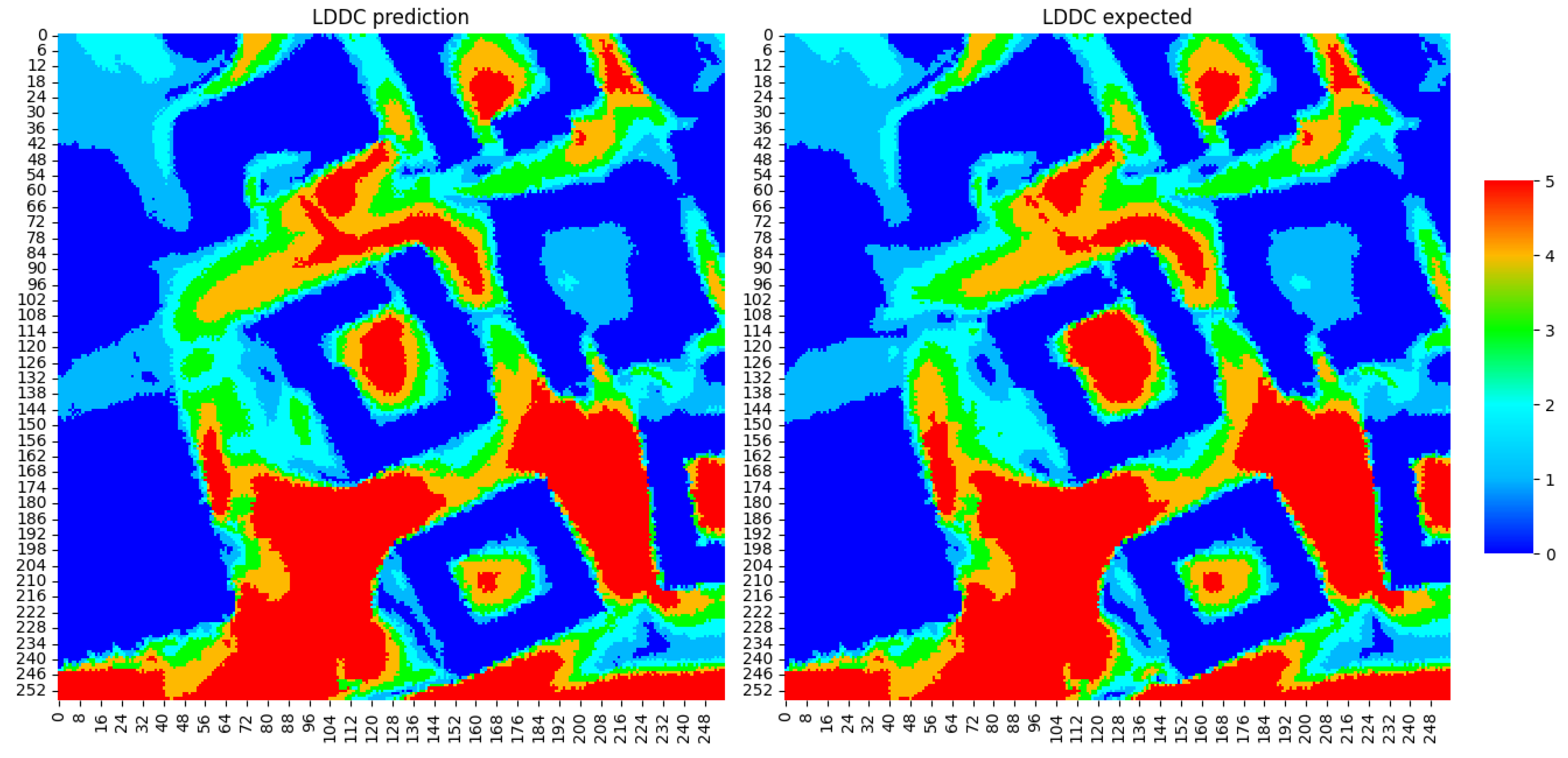
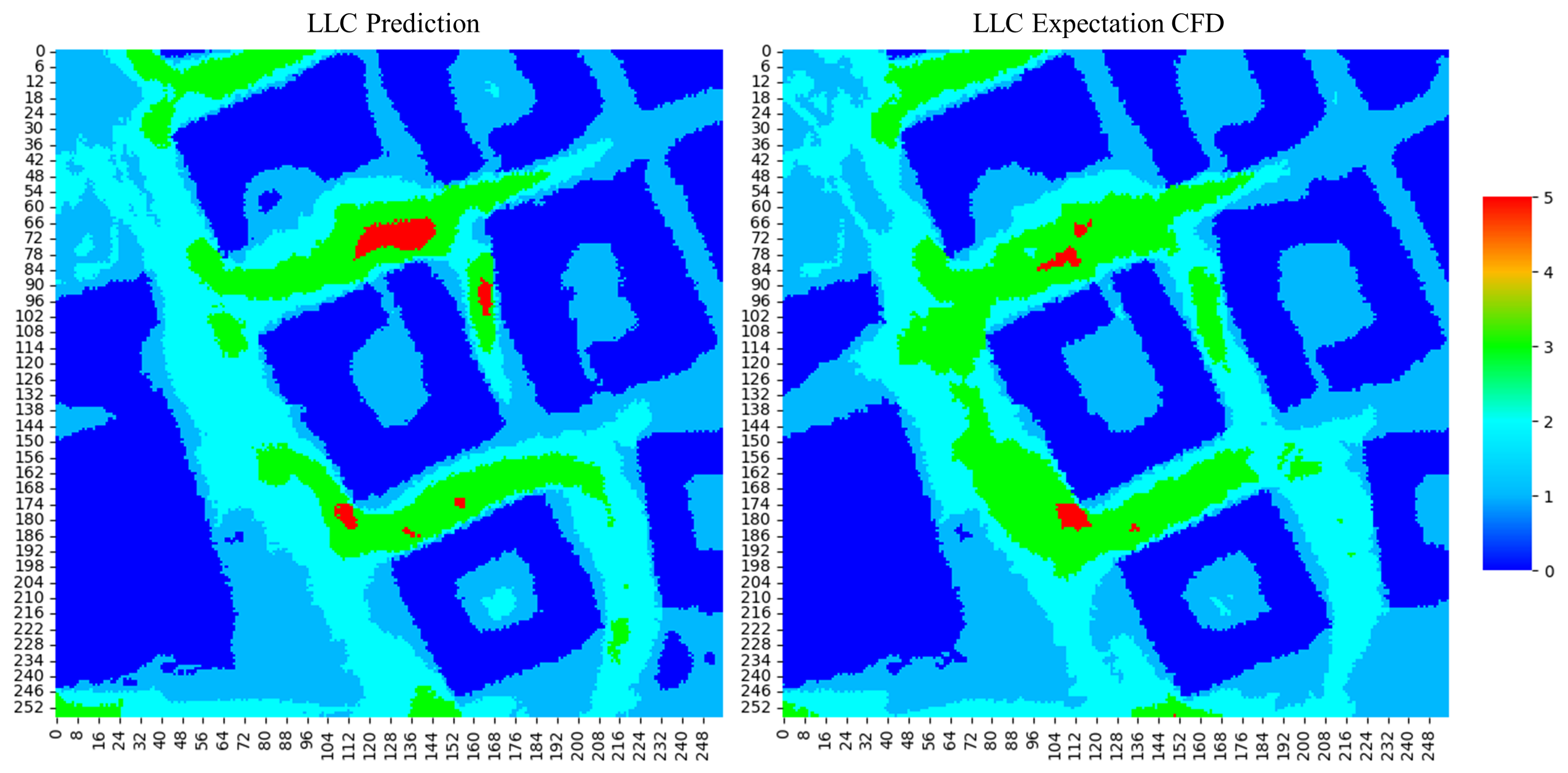
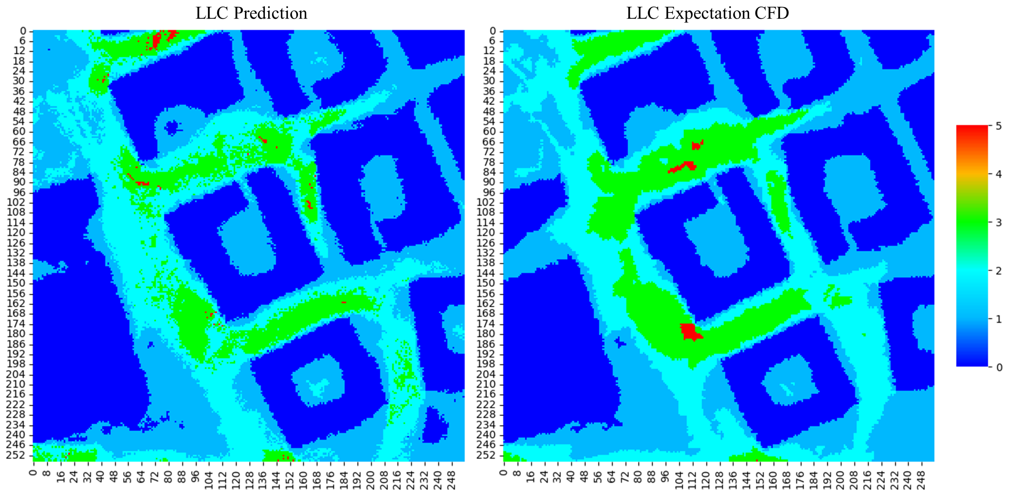
4.3.2. Classification Model

The performance of the classification model on the LLC test set is summarized in Table 8 under “Classification”. As for the regression model, the average F 1 -score per sample is again >80% for all models and is best for the “100 Simulations” model, with an F 1 -score of 82.75 %. It is only slightly higher than the average F 1 -score for the model “200 Simulations”, with a value of 82.15 %. The LLC was predicted with the trained decision tree classifier (see Section 3.5), which for the four different training data sets always yielded a score of at least 96% (see Section 4.2.3).
Again, the recall for each class is given separately in Table 8 under “Classification”.
Comparing these results with the regression model, one notices that classes 3 and 5 especially are worse for the classification model. The average recall for class 5 predictions decreased by 14.68 , 11.30 , and 18.01 percentage points for the “50 Simulations”, “100 Simulations”, and the “200 Simulations” models, respectively.
Training the DTC is an imbalanced data problem because there are significantly fewer data points of class 5 than of any other class. We summarize the number of pixels for each class, k, for the LLC test set in Appendix A, in Table A1. Because of this, we perform oversampling before training the DTC (see Section 4.2.3). For the training data of the classification model, on the other hand, this is not the case, because of the data augmentation strategy using the extreme case LLC (see Section 3.4). By using these extreme case LLCs, the higher the wind rose speed is, the higher the LLC is in the extreme case scenario. In this way, we can generate a data set that is not imbalanced.
Since the score on the test set of the decision tree classifier is, with more than 96%, high (see Table 7), the poorer predictions of class 5 therefore root in prediction errors of the classification model. In the test set, we observe that, as the wind rose speed of the extreme case scenario increases, the F 1 -score decreases. We observe a maximum deviation from the optimal F 1 -score of 36.65 % in the test set (see Figure 12). Since all 64 predictions for the extreme case scenarios are used for LLC prediction (some with a high F 1 -score, some with a comparably lower F 1 -score), this leads to the poorer predictions of class 5.
The comparison between prediction and expectation for test sample 4 is shown in Figure 15. On the left side, the prediction of the LLC by the “200 Simulations” model is shown, and, on the right side, the expected LLC calculated with the CFD solver is shown. This sample scores an F 1 -score of 83.14 %. The overall LLC is therefore predicted well. Classes 0, 1, and 2 yield a recall of 98.89 %, 79.40 %, and 68.83 %. The recall for class 3 equals 62.15 %, and the recall for class 5 equals 1.85 %. The other LLC test set samples are shown in Appendix A, in Figure A3 and Figure A4.

4.3.3. Summary

Overall, both the regression and the classification models yield promising results for LLC prediction. The regression model performs slightly better with respect to the average F 1 -score than the classification model. For both models, it is possible to predict the LLC with an F 1 -score of >80.0%, independent of the number of simulations used for the training set. However, our observation is that the more training data used for the regression model, the better is the prediction of the highest LLC class concerned with pedestrian safety. The models are trained independent of the wind statistic. Therefore, the LLC test step can be performed for different wind statistics. Furthermore, the regression model is even independent of the LLC calculation rule because it is trained on velocity magnitude.
Even though the models provide overall good predictions of the LLC, the highest class 5 of the LLC, which is concerned with pedestrian safety, is not predicted that well. Here, the recall for class 5 on average equals 19.84 % and 1.83 % for the regression and classification models, respectively. The regression model therefore performs better in predicting class 5, but neither model can make a reliable prediction for class 5. The prediction performance of class 5 could be improved by weighing the higher velocities more heavily in the regression model or by penalizing the inaccuracy of predicting class 5 by the classification model, but this was out of the scope of this paper.
The trained surrogate models have some limitations. Firstly, these models are trained on a specific use case and thus may not be applicable to a different topology. Using the surrogate models in an optimization process to enhance wind comfort for this specific use case would result in a significant speed-up per optimization step. The CFD solver takes approximately 26 h for a complete simulation, whereas the surrogate models only require seconds to predict wind comfort. However, it is important to note that there are limitations in terms of accuracy when utilizing the surrogate models, and a validating simulation would be necessary.

5. Conclusions

In this study, we have considered a specific building site and compared two different machine learning workflows (MLWs) predicting wind comfort (LLC). The first MLW implements a U-Net regression model predicting wind velocity for extreme case scenarios. From these extreme case results, the LLC is directly computed for a specific wind rose statistic. The second MLW is based on a U-Net classification model predicting extreme case LLCs. For a specific wind rose statistic, a decision tree classifier predicts the LLC from these extreme case LLCs. Overall, the proposed MLWs produce positive results, with both models demonstrating good predictive capabilities. Independent of the training size, both models yield an F 1 -score of over 80%. The regression model with an F 1 -score of 84.48 % has proven to be more accurate, which increases our confidence in its predictive ability. Although both models performed well in general, there is a need for improvement in the prediction of class 5, which is concerned with pedestrian safety. To address this, the loss function can be adjusted by either weighting the higher velocities more heavily in the regression model or penalizing the inaccuracy of predicting class 5 by the classification model. Compared with the wind comfort prediction using a CFD solver, the trained regression and classification models yield a result within seconds instead of 26 h. This leads to a significant speed-up in terms of wind comfort optimization.
An important feature of our methodology is the scenario-based data augmentation, which has allowed us to generate additional training data from existing simulations by a factor of 72 at most per simulation, leading to a maximum of 15,336 training samples. It is also worth noting that, thanks to this scenario-based approach, both models stand out for their independence from wind rose data. This quality takes us a step closer to achieving a higher degree of generalizability.
Overall, this study has provided valuable insights. Our study is limited to the use case we investigated in this work, and, as of now, it is not immediately possible to apply the trained model to different building sites. To extend the model’s utility to various building sites, a process of additional simulations and retraining would be necessary. In a real-world application, this procedure is not practical because it would require a large amount of computational resources and time. Also, our models do not incorporate the underlying physics of the processes we are modeling. Integrating physics into our models is a potential avenue for further improving predictive accuracy. While the current model’s application to different building sites may not be readily possible, it is essential to note that our research lays the foundation for potential future advancements.

Author Contributions

Conceptualization, J.W., D.N., F.H., T.J. and A.M.; methodology, J.W., D.N., F.H., T.J. and A.M.; software, J.W., D.N., F.H., T.J. and A.M.; validation, F.H.; formal analysis, J.W. and D.N.; investigation, J.W., D.N., F.H., T.J. and A.M.; resources, F.E.; data curation, J.W., D.N., F.H., T.J., A.M. and A.G. writing—original draft preparation, J.W., D.N. and F.H.; writing—review and editing, J.W., D.N., F.H., T.J., A.M. and A.G. visualization, J.W., D.N. and F.H.; supervision, D.N. and F.E.; project administration, D.N. and A.M.; funding acquisition, A.M. and F.E. All authors have read and agreed to the published version of the manuscript.

Funding

This work is part of the Digital Twin Cities Centre supported by Sweden’s Innovation Agency Vinnova under Grant No. 2019-00041. This work was further supported by the Swedish Research Council for Sustainable Development Formas under the grants 2019-01169 and 2019-01885. The computations were enabled by resources provided by the Swedish National Infrastructure for Computing (SNIC) at HPC2N partially funded by the Swedish Research Council through grant agreement no. 2018-05973.

Data Availability Statement

The simulation data presented in this study are available on request from the corresponding authors.

Conflicts of Interest

The authors declare no conflicts of interest.

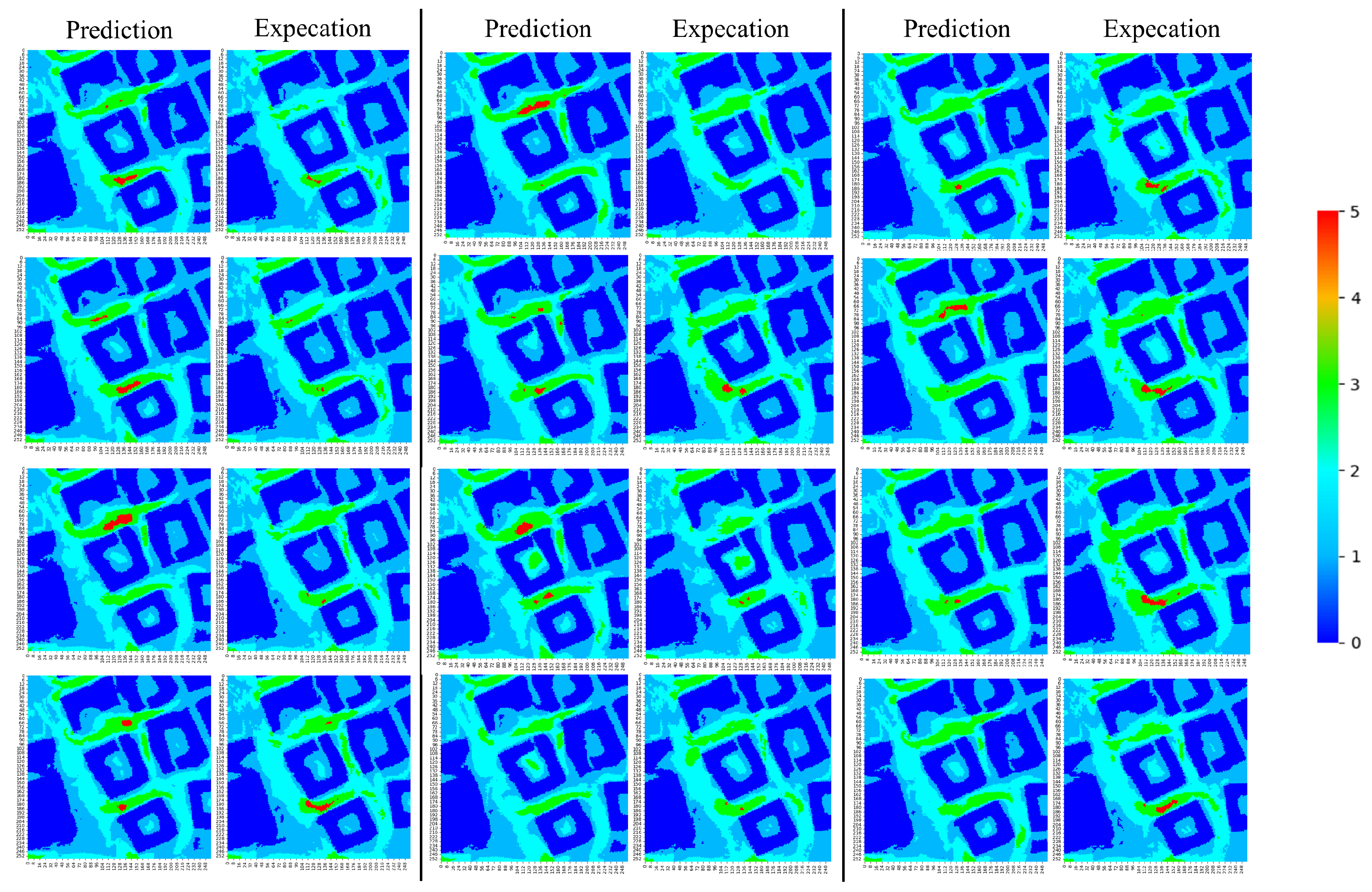
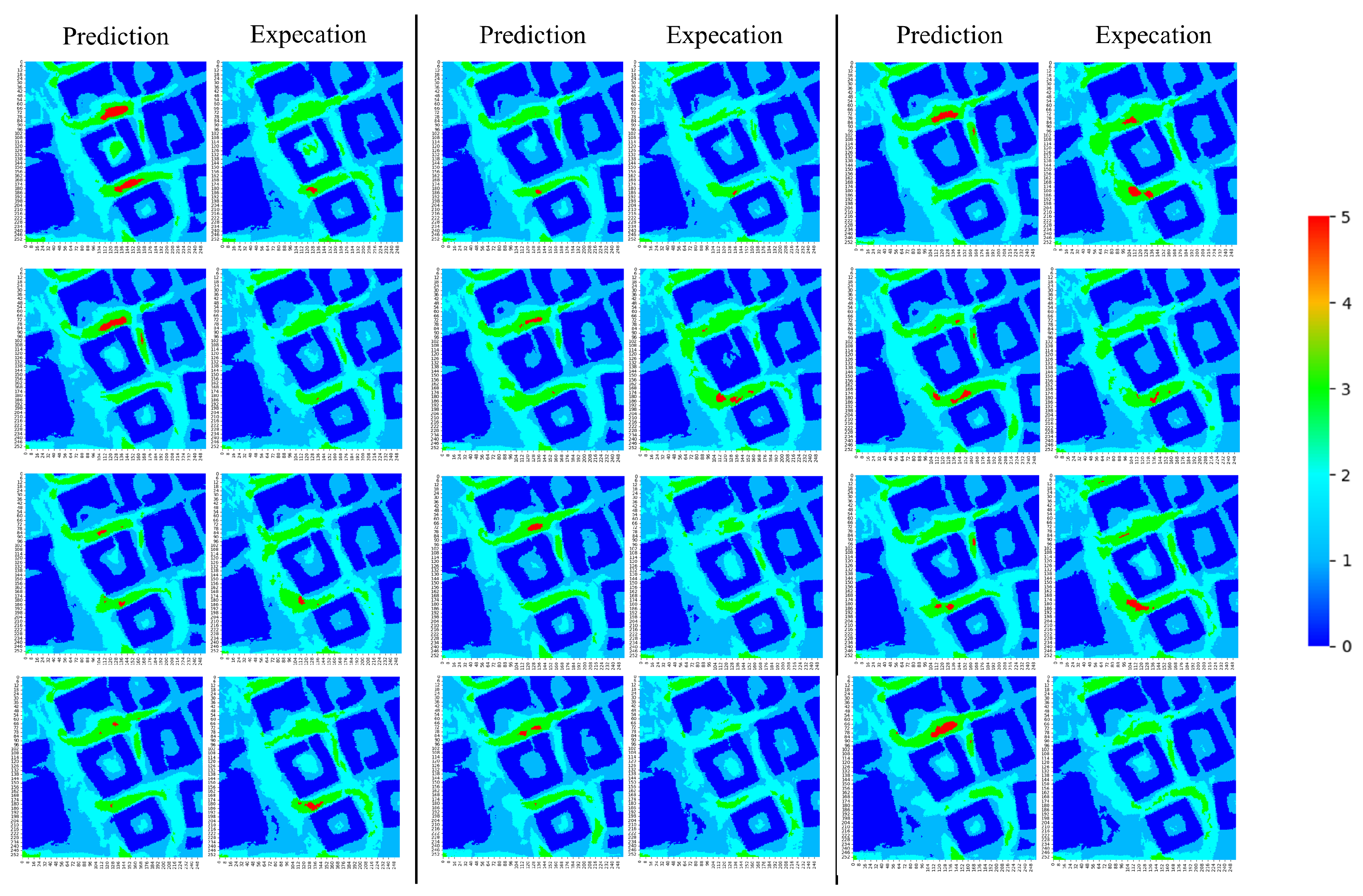
Appendix A. LLC Test Set

Table A1. Number of pixels per class for each test sample in the LLC test set.
Sample No.Class 0Class 1Class 2Class 3Class 4Class 5
127,92921,01814,8052391030
227,31121,93613,0953171023
327,16220,42414,1313808011
426,20719,53712,75368770162
527,15820,21614,05638870219
626,98820,63014,158376000
727,11619,29414,32846920106
827,11521,86413,8002728029
927,20819,97614,6603668024
1026,88919,81014,88438520101
1126,40219,05314,40654640211
1226,48618,94013,69561880227
1327,19920,14314,62434470123
1426,64019,54114,6954579081
1527,25120,55813,943378400
1627,26019,90514,345373053
1726,96419,65614,97538130128
1827,24320,66114,775285106
1927,59219,11113,10455370192
2027,31820,71614,73726500
2127,94121,92613,478219100
2226,83619,52713,17357350265
2327,08019,94213,8744610030
2426,58819,11413,96456760194
2527,65220,89413,846314400
Figure A1. LLC prediction by regression model for the test samples in LLC test set; on the left side of each column is the prediction and on the right side of each column the expectation is shown; part 1.
Make 06 00006 g0a1
Figure A2. LLC prediction by regression model for the test samples in LLC test set; on the left side of each column is the prediction and on the right side of each column the expectation is shown; part 2.
Make 06 00006 g0a2
Figure A3. LLC prediction by classification model for the test samples in LLC test set; on the left side of each column is the prediction and on the right side of each column the expectation is shown; part 1.
Make 06 00006 g0a3
Figure A4. LLC prediction by classification model for the test samples in LLC test set; on the left side of each column is the prediction and on the right side of each column the expectation is shown; part 2.
Make 06 00006 g0a4

References

  1. Lawson, T.V. The effect of wind on people in the vicinity of buildings. In Proceedings of the 4th International Conference on Wind Effects on Buildings and Structures, London, UK, September 1975. [Google Scholar]
  2. Allegrini, J. A wind tunnel study on three-dimensional buoyant flows in street canyons with different roof shapes and building lengths. Build. Environ. 2018, 143, 71–88. [Google Scholar] [CrossRef]
  3. Blocken, B.; Janssen, W.D.; van Hooff, T. CFD simulation for pedestrian wind comfort and wind safety in urban areas: General decision framework and case study for the Eindhoven University campus. Environ. Model. Softw. 2012, 30, 15–34. [Google Scholar] [CrossRef]
  4. Fadl, M.S.; Karadelis, J. CFD Simulation for Wind Comfort and Safety in Urban Area: A Case Study of Coventry University Central Campus. Int. J. Archit. Eng. Constr. 2013, 2, 131–143. [Google Scholar] [CrossRef]
  5. Zheng, C.; Li, Y.; Wu, Y. Pedestrian-level wind environment on outdoor platforms of a thousand-meter-scale megatall building: Sub-configuration experiment and wind comfort assessment. Build. Environ. 2016, 106, 313–326. [Google Scholar] [CrossRef]
  6. Wu, H.; Kriksic, F. Designing for pedestrian comfort in response to local climate. J. Wind Eng. Ind. Aerodyn. 2012, 104–106, 397–407. [Google Scholar] [CrossRef]
  7. Willemsen, E.; Wisse, J.A. Design for wind comfort in The Netherlands: Procedures, criteria and open research issues. J. Wind Eng. Ind. Aerodyn. 2007, 95, 1541–1550. [Google Scholar] [CrossRef]
  8. Düring, S.; Chronis, A.; Koenig, R. Optimizing Urban Systems: Integrated optimization of spatial configurations. In Proceedings of the 11th Annual Symposium on Simulation for Architecture and Urban Design, Vienna, Austria, 25–27 May 2020. [Google Scholar]
  9. Purup, P.B.; Petersen, S. Research framework for development of building performance simulation tools for early design stages. Autom. Constr. 2020, 109, 102966. [Google Scholar] [CrossRef]
  10. Lino, M.; Fotiadis, S.; Bharath, A.A.; Cantwell, C.D. Current and emerging deep-learning methods for the simulation of fluid dynamics. Proc. R. Soc. A Math. Phys. Eng. Sci. 2023, 479, 20230058. [Google Scholar] [CrossRef]
  11. Ronneberger, O.; Fischer, P.; Brox, T. U-Net: Convolutional Networks for Biomedical Image Segmentation. In Medical Image Computing and Computer-Assisted Intervention—MICCAI 2015; Navab, N., Hornegger, J., Wells, W.M., Frangi, A.F., Eds.; Lecture Notes in Computer Science; Springer International Publishing: Cham, Switzerland, 2015; Volume 9351, pp. 234–241. [Google Scholar] [CrossRef]
  12. Farimani, A.B.; Gomes, J.; Pande, V.S. Deep Learning the Physics of Transport Phenomena. arXiv 2017, arXiv:1709.02432. [Google Scholar]
  13. Thuerey, N.; Weissenow, K.; Prantl, L.; Hu, X. Deep Learning Methods for Reynolds-Averaged Navier-Stokes Simulations of Airfoil Flows. AIAA J. 2020, 58, 25–36. [Google Scholar] [CrossRef]
  14. Low, S.J.; Raghavan, V.S.G.; Gopalan, H.; Wong, J.C.; Yeoh, J.; Ooi, C.C. FastFlow: AI for Fast Urban Wind Velocity Prediction. In Proceedings of the 2022 IEEE International Conference on Data Mining Workshops (ICDMW), Orlando, FL, USA, 28 November–1 December 2022. [Google Scholar]
  15. Isola, P.; Zhu, J.Y.; Zhou, T.; Efros, A.A. Image-to-Image Translation with Conditional Adversarial Networks. In Proceedings of the IEEE Conference on Computer Vision and Pattern Recognition (CVPR), Honolulu, HI, USA, 21–26 July 2017. [Google Scholar]
  16. Mokhtar, S.; Sojka, A.; Davila, C.C. Conditional Generative Adversarial Networks for Pedestrian Wind Flow Approximation; Society for Modeling & Simulation International (SCS): San Diego, CA, USA, 2020. [Google Scholar]
  17. BenMoshe, N.; Fattal, E.; Leitl, B.; Arav, Y. Using Machine Learning to Predict Wind Flow in Urban Areas. Atmosphere 2023, 14, 990. [Google Scholar] [CrossRef]
  18. Eslamirad, N.; de Luca, F.; Sakari Lylykangas, K.; Ben Yahia, S. Data generative machine learning model for the assessment of outdoor thermal and wind comfort in a northern urban environment. Front. Archit. Res. 2023, 12, 541–555. [Google Scholar] [CrossRef]
  19. Mostafa, K.; Zisis, I.; Moustafa, M.A. Machine Learning Techniques in Structural Wind Engineering: A State-of-the-Art Review. Appl. Sci. 2022, 12, 5232. [Google Scholar] [CrossRef]
  20. Hoeiness, H.; Gjerde, K.; Oggiano, L.; Giljarhus, K.E.T.; Ruocco, M. Positional Encoding Augmented GAN for the Assessment of Wind Flow for Pedestrian Comfort in Urban Areas. arXiv 2021, arXiv:2112.08447. [Google Scholar]
  21. SMHI. Available online: https://www.smhi.se/data/meteorologi/ladda-ner-meteorologiska-observationer/#param=wind,stations=core,stationid=71420 (accessed on 2 October 2023).
  22. The City of London Corporation Wind Microclimate Guidelines for Developments in the City of London. 2019; pp. 1–15. Available online: https://www.cityoflondon.gov.uk/assets/Services-Environment/wind-microclimate-guidelines.pdf (accessed on 15 November 2023).
  23. Girin, A.; Lawson Wind Comfort Criteria: A Closer Look. Simscale Blog. 2021. Available online: https://www.simscale.com/blog/lawson-wind-comfort-criteria/ (accessed on 25 October 2022).
  24. Mark, A.; Rundqvist, R.; Edelvik, F. Comparison Between Different Immersed Boundary Conditions for Simulation of Complex Fluid Flows. Fluid Dyn. Mater. Process. 2011, 7, 241–258. [Google Scholar] [CrossRef]
  25. Mitkov, R.; Pantusheva, M.; Naserentin, V.; Hristov, P.; Wästberg, D.; Hunger, F.; Mark, A.; Petrova-Antonova, D.; Edelvik, F.; Logg, A. Using the Octree Immersed Boundary Method for urban wind CFD simulations. IFAC-PapersOnLine 2022, 55, 179–184. [Google Scholar] [CrossRef]
  26. Vanky, P.; Mark, A.; Haeger-Eugensson, M.; Tarraso, J.; Adelfio, M.; Kalagasidis, A.S.; Sardina, G. Addressing wind comfort in an urban area using an immersed boundary framework. Tech. Mech. 2023, 43, 151–161. [Google Scholar] [CrossRef]
  27. Andersson, T.; Nowak, D.; Johnson, T.; Mark, A.; Edelvik, F.; Küfer, K.H. Multiobjective Optimization of a Heat-Sink Design Using the Sandwiching Algorithm and an Immersed Boundary Conjugate Heat Transfer Solver. J. Heat Transf. 2018, 140, 102002. [Google Scholar] [CrossRef]
  28. Nowak, D.; Johnson, T.; Mark, A.; Ireholm, C.; Pezzotti, F.; Erhardsson, L.; Ståhlberg, D.; Edelvik, F.; Küfer, K.H. Multicriteria Optimization of an Oven With a Novel ϵ-Constraint-Based Sandwiching Method. J. Heat Transf. 2020, 143. [Google Scholar] [CrossRef]
  29. Nowak, D.; Werner, J.; Parsons, Q.; Johnson, T.; Mark, A.; Edelvik, F. Optimisation of city structures with respect to high wind speeds using U-Net models. Eng. Appl. Artif. Intell. Under Rev. 2024; in press. [Google Scholar]
  30. Brozovsky, J.; Simonsen, A.; Gaitani, N. Validation of a CFD model for the evaluation of urban microclimate at high latitudes: A case study in Trondheim, Norway. Build. Environ. 2021, 205, 108175. [Google Scholar] [CrossRef]
  31. Wieringa, J. Updating the Davenport roughness classification. J. Wind Eng. Ind. Aerodyn. 1992, 41, 357–368. [Google Scholar] [CrossRef]
  32. Aupoix, B. Roughness Corrections for the k–ω Shear Stress Transport Model: Status and Proposals. J. Fluids Eng. 2014, 137, 021202. [Google Scholar] [CrossRef]
  33. Kalitzin, G.; Medic, G.; Iaccarino, G.; Durbin, P. Near-wall behavior of RANS turbulence models and implications for wall functions. J. Comput. Phys. 2005, 204, 265–291. [Google Scholar] [CrossRef]
  34. Menter, F.R. Two-Equation Eddy-Viscosity Turbulence Models for Engineering Applications. AIAA J. 1994, 32, 1598–1605. [Google Scholar] [CrossRef]
  35. Menter, F.R.; Kuntz, M.; Langtry, M.R. Ten Years of Industrial Experience with the SST Turbulence Model. Turbul. Heat Mass Transf. 1994, 4, 625–632. [Google Scholar]
  36. Sobol’, I.M. On the distribution of points in a cube and the approximate evaluation of integrals. Zhurnal Vychislitel’noi Mat. Mat. Fiz. 1967, 7, 784–802. [Google Scholar] [CrossRef]
  37. Stoller, D.; Ewert, S.; Dixon, S. Wave-U-Net: A Multi-Scale Neural Network for End-to-End Audio Source Separation. arXiv 2018, arXiv:1806.03185. [Google Scholar]
  38. Zhang, Z.; Liu, Q.; Wang, Y. Road Extraction by Deep Residual U-Net. IEEE Geosci. Remote Sens. Lett. 2018, 15, 749–753. [Google Scholar] [CrossRef]
  39. Giri, R.; Isik, U.; Krishnaswamy, A. Attention Wave-U-Net for Speech Enhancement. In Proceedings of the 2019 IEEE Workshop on Applications of Signal Processing to Audio and Acoustics (WASPAA), Piscataway, NJ, USA, 20–23 October 2019. [Google Scholar] [CrossRef]
  40. Paszke, A.; Gross, S.; Massa, F.; Lerer, A.; Bradbury, J.; Chanan, G.; Killeen, T.; Lin, Z.; Gimelshein, N.; Antiga, L.; et al. PyTorch: An Imperative Style, High-Performance Deep Learning Library. In Advances in Neural Information Processing Systems 32; Curran Associates, Inc.: New York, NY, USA, 2019; pp. 8024–8035. [Google Scholar]
  41. Goodfellow, I.; Bengio, Y.; Courville, A. Deep Learning; MIT Press: Cambridge, MA, USA, 2016; Available online: http://www.deeplearningbook.org (accessed on 10 October 2023).
  42. Hastie, T.; Tibshirani, R.; Friedman, J.H. The Elements of Statistical learning: Data Mining, Inference, and Prediction/Trevor Hastie, Robert Tibshirani, Jerome Friedman, 2nd ed.; Springer Series in Statistics; Springer: New York, NY, USA, 2009. [Google Scholar]
  43. Pedregosa, F.; Varoquaux, G.; Gramfort, A.; Michel, V.; Thirion, B.; Grisel, O.; Blondel, M.; Prettenhofer, P.; Weiss, R.; Dubourg, V.; et al. Scikit-learn: Machine Learning in Python. J. Mach. Learn. Res. 2011, 12, 2825–2830. [Google Scholar]
  44. Rebala, G.; Ravi, A.; Churiwala, S. An Introduction to Machine Learning; Springer International Publishing: Cham, Switzerland, 2019. [Google Scholar] [CrossRef]
  45. Akiba, T.; Sano, S.; Yanase, T.; Ohta, T.; Koyama, M. Optuna: A Next-generation Hyperparameter Optimization Framework. In Proceedings of the Proceedings of the 25th ACM SIGKDD International Conference on Knowledge Discovery and Data Mining, Anchorage, AK, USA, 4–8 August 2019. [Google Scholar]
  46. Krawczyk, B. Learning from imbalanced data: Open challenges and future directions. Prog. Artif. Intell. 2016, 5, 221–232. [Google Scholar] [CrossRef]
  47. Lemaître, G.; Nogueira, F.; Aridas, C.K. Imbalanced-learn: A Python Toolbox to Tackle the Curse of Imbalanced Datasets in Machine Learning. J. Mach. Learn. Res. 2017, 18, 1–5. [Google Scholar]
Figure 1. The study area studied in this paper; (a) shows the entire study area, and the smaller blue square box is the area we are considering for the ML model; (b) shows the location of the computational box; (c) shows an enlargement of the area we are considering for the ML model (blue square box); and (d) shows an example of a building design for the new building (red boxes).
Make 06 00006 g001
Figure 2. (a) illustrates the corresponding wind rose of the study area; and (b) displays the LLC for a sample simulation.
Make 06 00006 g002
Figure 3. Example of LLC for (a) the wind rose statistic in Equation (2), (b) extreme case LLC based on wind rose statistics W ( 0.5   m / s , 0.0 ° ) and leads to a low wind comfort, and (c) the extreme case LLC based on W ( 14   m / s , 315 ° ) and leads to a high wind comfort.
Make 06 00006 g003
Figure 4. Velocity distribution of three different grids; from left to right: 2.7 million cells with a local resolution of 1.2 m in the vertical direction, 6 million cells with a local resolution of 0.6 m in the vertical direction, and 21 million cells with a local resolution of 0.3 m in the vertical direction, indicating visually the differences in the velocity magnitude when applying different meshes, needed to evaluate grid convergence.
Make 06 00006 g004
Figure 5. (a) Architecture of the CNN; and (b) outputs of the CNN depending on the regression or classification task.
Make 06 00006 g005
Figure 6. Example of an unnormalized training sample with the inputs (1)–(3) and the output for regression and classification; the regression output is the velocity magnitude in m/s, and the classification output is the extreme case LLC (see Section 2.2).
Make 06 00006 g006
Figure 7. Training data for decision tree classifier for predicting LLC for the wind rose statistic, W, based on the extreme case LLC of the classification model, illustrated for the post-processed/predicted data of one simulation.
Make 06 00006 g007
Figure 8. ML workflow (MLW) for prediction: Step 1a illustrates the MLW for the regression model; and Step 1b shows the MLW for the classification model.
Make 06 00006 g008
Figure 9. Validation loss for the regression model trained on three different training sets.
Make 06 00006 g009
Figure 10. Performance on test set of the three trained regression models; (a) shows a line plot for different quantiles of the test set; and (b) shows the distribution of the test set in the form of a box plot.
Make 06 00006 g010
Figure 11. Validation loss for the classification model trained on three different training sets.
Make 06 00006 g011
Figure 12. Performance on test set of the three trained regression models with respect to the deviation from the ideal F 1 -score; (a) shows a line plot for different quantiles of the test set; and (b) shows the distribution of the test set in the form of a box plot.
Make 06 00006 g012
Figure 13. Example of an test sample predicted with model “200 Simulations”; on the left side the prediction of the extreme case LLC is shown and on the right side the expectation is shown.
Make 06 00006 g013
Figure 14. LLC prediction (left) of regression model for test sample 4 compared with the expected LLC from the CFD solver (right).
Make 06 00006 g014
Figure 15. LLC prediction (left) of classification model for test sample 4 compared with the expected LLC from the CFD solver (right).
Make 06 00006 g015
Table 1. Dimensions and positions for each segment of the new building block.
SegmentWidthLengthx Positiony Positionz PositionRotation about z-Axis
1 22.15 m 13.0 m 92.98 m 46.07 m 9.0 m 25.8 °
2 9.0 m 12.0 m 109.23 m 40.44 m 9.0 m 115.8 °
3 19.25 m 12.0 m 103.08 m 27.73 m 9.0 m 115.8 °
4 22.85 m 12.6 m 74.67 m 59.89 m 9.0 m 25.8 °
5 25.1 m 12.0 m 61.58 m 42.28 m 9.0 m 115.8 °
6 10.0 m 12.0 m 59.52 m 20.34 m 9.0 m 25.8 °
7 10.0 m 12.0 m 50.52 m 24.69 m 9.0 m 25.8 °
8 20.1 m 11.6 m 94.7 m 9.92 m 9.0 m 115.8 °
9 25.4 m 12.0 m 74.92 m 11.51 m 9.0 m 25.8 °
Table 2. Lawson LDDC criterion.
ClassUpper Velocity Limit in m/sExceedance ThresholdComfort Level
A-02.5<5Frequent sitting
B-14<5Occasional sitting
C-26<5Standing
D-38<5Walking
E-48>5%Uncomfortable
S-515>0.022%Unsafe
Table 3. Hyperparameters of CNN. * was solely used for the regression model.
HyperparameterRange/Set
channel exponent { 2 , 3 , 4 , 5 , 6 , 7 , 8 } *
dropout probability [ 0.0 , 1.0 ]
batch size { 1 , 6 , 11 , , 46 }
maximum learning rate [ 0.0001 , 0.01 ]
decaying learning rate { True , False }
Table 4. Optimal hyperparameters for training of the regression models.
Setting50 Simulations100 Simulations200 Simulations
channel exponent L in Equation (6)788
dropout probability 0.07002 0.02510 0.06860
batch size666
maximum learning rate 0.00108 0.00076 0.00077
decaying learning rateTrueTrueTrue
trainable parameters36,668,929146,607,105146,607,105
number of training samples4536813615,336
Table 5. Optimal hyperparameters for training of the classification models.
Setting50 Simulations100 Simulations200 Simulations
channel exponent777
dropout probability 0.02185 0.03889 0.00087
batch size61611
maximum learning rate 0.00013 0.005155 0.00328
decaying learning rateTrueTrueTrue
trainable parameters36,689,41436,668,92936,689,414
number of training samples4032723213,632
Table 6. Hyperparameters of DTC.
HyperparameterRange/Set
maximum depth of the tree { 5 , 8 , 11 , 14 , 17 , 20 , 23 , 26 , 29 , 32 , 35 }
min. number of samples leaf { 2 , 4 , 6 , , 16 , 18 , 20 }
Optimal Hyperparameters
maximum depth of the tree35
min. number of samples leaf2
Table 7. Accuracy of DTC for each training set.
Setting50 Simulations100 Simulations200 Simulations
Accuracy in %96.7696.5296.12
Table 8. Performance of the regression and classification models on the LLC test set.
Metric50 Simulations100 Simulations200 Simulations
Regression
Average F 1 -score Regression 0.8347 0.8406 0.8448
Recall class 0 0.9740 0.9760 0.9774
Recall class 1 0.7990 0.8173 0.7950
Recall class 2 0.6772 0.6946 0.7188
Recall class 3 0.6634 0.6252 0.6824
Recall class 5 0.2659 0.1222 0.1984
Classification
Average F 1 -score Classification 0.8085 0.8270 0.8256
Recall class 0 0.9756 0.9777 0.9792
Recall class 1 0.7571 0.7759 0.7854
Recall class 2 0.6149 0.6896 0.6519
Recall class 3 0.6518 0.5799 0.6403
Recall class 5 0.1191 0.0092 0.0183
Disclaimer/Publisher’s Note: The statements, opinions and data contained in all publications are solely those of the individual author(s) and contributor(s) and not of MDPI and/or the editor(s). MDPI and/or the editor(s) disclaim responsibility for any injury to people or property resulting from any ideas, methods, instructions or products referred to in the content.

